

1 Introduction
During the last 70 years, population ecologists have been debating hotly on whether intrinsic or extrinsic factors are more relevant in generating a population dynamical pattern, and the majority of the hypothesis advanced on this respect have been tested on both theoretical and experimental grounds [1,2]. However, and somewhat paradoxically, most of the major theoretical and empirical advances within this field have been derived with the time-series analysis of fluctuations of natural, unmanipulated populations, and the use of autoregressive (AR) models and its extensions has been key during this development (see, e.g., [3–7]). The use of AR models is justified by the fact that the trajectory of a population through time can be described as a dynamic system with some kind of feedback in population size [8]. Thus, most authors (e.g., [8,9]) have advocated the use of direct and/or delayed difference equations, which take the general, deterministic form:
| (1) |
| (2) |
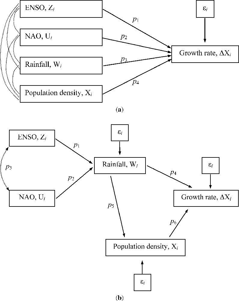
Graphs depicting two possible topological relationships between a set of ecological and climatic variables. In (a), the standard autoregressive model with environmental covariates is shown as an unstructured path model; the dotted arcs connecting the set of covariates represent unresolved relationships. A simple topological transformation (b) allow a more realistic depiction of the relationships between the set of variables in (a), yielding a structured path model. SEM deals with the kind of models represented in (b). In both figures, variables represent time-independent stochastic variation, and each stand for a parameter. The direction of arrows indicates the direction of causation (a doubled-headed arrow denote a simultaneous covariation).
See Fig. 1a for a visual depiction of the relationships between the variables in Eq. (2). However its simplicity and generality, several caveats underlie this modelling procedure. First, Eq. (2) implicitly assumes that there is no temporal correlation in (specifically, that it describes a white noise process with constant variance [8,16]); nevertheless, Moran [17], when analysing the time series of Canadian lynx fur returns with an AR model [16], was the first to note that this assumption would not hold in many cases (see also [3,16]). Indeed, the introduction of autocorrelation in any covariate has been shown to increase the magnitude of statistical density dependence [18–20]. Second, the presence of multicollinearity among the set of covariates inflates the variance of individual parameter estimates (the so-called variance inflation effect; [21]). Third, the presence of measurement error (e.g., sampling variability) tends to distort the estimate of parameters and associated uncertainties [19]. And fourth, the inclusion of nonadditive effects of climate on the dynamics [11] is severely limited within the framework of Eq. (2).
In recent years, several modelling approaches, such as state-based models [22,23] and variance components methods [24–26] have been proposed in order to overcome the effects of sampling variance and coloured residuals on population models. Nevertheless, both the role of multicollinearity and the statistical modelling of nonadditive climatic effects have been seldom explored (see [11,21]). In the present paper, a modelling procedure is described that is able to simultaneously circumvent the problems outlined above. Indeed, it has been recently applied to study the dynamics of a globally threatened bird, with successful results [27,28]. The technique, known as Structural Equation Modelling (hereafter SEM), was originally proposed by the evolutionary biologist Sewall Wright [29,30] as a path analysis method, and was later developed by econometricians, sociologists, and artificial intelligence researchers [31]. In a first part, the concepts, philosophy and methodology underlying SEM will be briefly outlined and placed in an ecological time-series perspective. In order to illustrate the potential of the procedure, an ecological example will be presented in a second part along with real data, and the advantages and limitations of SEM relative to traditional techniques will be highlighted in a final section.
2 Preliminary concepts
2.1 Path analysis
Wright [29] was the first to propose a method to partition both direct and indirect relationships among a set of variables, latter called path analysis [30]. Sociologist, econometricians and artificial intelligence researchers have been using path analyses and its extensions ever since the fifties and sixties [32,33]. However, it was not until the seventies when biologist first used path analysis in both experimental and observational approaches (see [33–36] for reviews). Indeed, in addition to Wright it was Haavelmo [37], an econometrician, who made the first attempt to lay down the foundations of the vast and growing field of SEM.
Path analysis, and associated path diagrams, can be regarded as a first step in SEM [38,39]. Path analysis allow the construction of a set of mathematical equations describing the patterns of covariance among a set of variables, as proposed by a substantive (verbal) hypothesis. The visual depiction of a path analysis is called a path diagram (see Fig. 1b for an example). The parameters of individual covariances (or correlations) are then estimated while holding the rest of variables constant [33]; if this estimation is done on standardized variables, the correlations are interpreted as standardized partial regression coefficients (indeed, multiple regression can be regarded as a special, unstructured version of path analysis; [31,33]). Examples of the current use of path analysis in biology include the study of complex patterns of selection on phenotypic traits [34,36], and the examination of direct and indirect effects in dynamic interaction webs [40–42].
2.2 The Structural Equation Model
The language of SEM requires the notion of latent variable [31]. Every observation of a natural phenomenon is imperfect, and is made with some measurement error. Thus, an observed (manifest) variable, such as the abundance estimates obtained through stratified transects, is always an indicator of some unobserved (latent) random variable (the true abundance; also known as factor or construct). If we consider that the correlation between the latent variables and its indicators are perfect (i.e., there is no measurement error), we have a path model [33]. Nevertheless, these correlations are probably never perfect, so we need a measurement model relating the set of indicators to each latent variable. That is, a measurement model specifies the structural model connecting the set of latent variables to one or more indicators [31]. If we further assume some kind of causal relationships between the set of latent variables, we have a full structural equations model [31,33,43]. Thus, a SEM is just the combination of a measurement model (the set of indicator variables and their errors) and a structural model (the set of latent constructs). This definition can be represented algebraically [31,43]. Be η a vector containing the endogenous constructs (e.g., population density and growth rate; see Fig. 1b), and be ξ a vector containing the exogenous constructs (e.g., large-scale climatic anomalies); additionally, be ζ a vector of errors on the endogenous constructs. The connection between these three vectors can be represented as the canonical structural equation for latent variables [31]:
| (3) |
The use of SEM, with its explicit distinction between latent and indicator variables, has been particularly scarce in ecological and evolutionary research ([27]; but see [44] for an early example). Myers and Cadigan [24,25] and Fromentin et al. [26] propose a variance-component method to estimate the effects of population density at different vital stages and stochasticity on the regulation of fish populations; although these authors did not explicitly state it, this method is essentially a SEM, but, given that their model is just-identified, there are no degrees of freedom left to estimate the goodness of fit of their model to the theoretical one expected given their data (see [28,41,45] for similar ecological examples, and see below).
2.3 Causality
Both path analysis and SEM are directly related to the somewhat controversial notion of causality [32]. Indeed, besides the less used Neyman–Rubin's potential response model, SEM stands out as the main language of causality [32]. However, scientists in general, and philosophers and statisticians in particular, have been largely aware of providing a clear definition of causality ([32,46,47] for ecological examples), but several attempts have been made to axiomise it [33,38]. Thus, for a relationship to be considered causal, four conditions should de met [33,38]. First, it must be transitive, in the sense that if a variable A causes B, and B causes C, then A must necessarily cause C. Second, the relationship must obey the Markov condition, by which the relationship impose the restriction that the response of C to A is impossible if the response of B to A is blocked. Third, events must be irreflexive, that is, a variable cannot cause itself. And fourth, the relationship must be asymmetric: if A causes B, B cannot simultaneously cause A (unless there are temporal feedbacks). Although some of these conditions might seem trivial, they are usually forgotten in ecological modelling. For instance, Stenseth et al. [13] recently suggested that the use of proxy indexes of large-scale climate in population dynamic studies provide the advantage of summarizing in a single measure the complex spatio-temporal variability of local weather. Nonetheless, it should never be forgotten that a biological population (C) is only affected by local weather (B), which in turn is a function of large-scale climate (A). Since the relationship between local and large-scale climate is usually nonstationary and nonlinear [13,48], this point should never be neglected. Finally, it should be noted that the notion of causality in this context must be held probabilistically [46], in the sense that a relationship is said to be causal because there is a propensity [49] for the effect to follow the cause. This axiom of causality is thus very important if we are to provide meaningful models describing the dynamics of natural populations.
3 Methods
3.1 Stages in Structural Equation Modelling
In this section the main steps involved in the construction of a structural equation model will be described briefly, and in the next section an ecological example will be presented to illustrate more clearly the matter. At a first stage, a useful philosophical frame in SEM is that of Chow [50] regarding the steps involved in a scientific investigation. Thus, as in many other areas of scientific research, the building of a SEM begins with the construction of a substantive (verbal) hypothesis concerning the natural phenomenon under study. Indeed, this is probably the most important step in SEM, because the following steps will depend upon the assumptions made by the verbal hypothesis. For instance, a sound knowledge of the natural history of a given species will allow us to construct a meaningful SEM and adopt the confirmatory approach, otherwise we should use the exploratory approach to find the topology that more plausibly captures the structure of covariance underlying our data (see [33–35,38,51] for controversies; see also Section 5). Once we have constructed the verbal hypothesis, we initiate the specification stage. Overall, at this stage we must specify the following [31]: relationship between latent variables; relationships between latent constructs and their indicators; functional forms of these relationships, and distributional assumptions. The next step is the identification of the model; at this stage, we must estimate the degrees of freedom (d.f.) of the SEM, calculated as the difference in the number of variances and covariances in the model and the number of free parameters to estimate. Thus, a model with d.f. = 0 is just-identified (that is, the model is just as complex as reality), and we cannot estimate the fit of the observed matrix to the theoretically expected given the causal structure [31]; only when d.f. > 0 can we estimate the fit, and in this case the model is said to be over-identified. After the identification stage we initiate the estimation of model parameters.
3.2 The fundamental hypothesis of SEM
At this stage, the fundamental hypothesis in SEM is introduced as:
| (4) |
3.3 Covariances or correlations?
Although SEM techniques are also known as Covariance Structure Modelling (CVM, [31]), it is sometimes useful to estimate correlations among variables, rather than covariances. For instance, when a model is scale-invariant and individual parameters are scale free (e.g., after standardisation), correlations will not alter the structure of the model, and standard errors for parameters will be unbiased [56,57]. Therefore, Browne [56] suggested corrections for standard errors based on the Constrained Estimation Theory. The use of correlations is suggested in population modelling since they represent partial regression coefficients when calculated on standardised variables (but see [32]; see also Section 2.1), thus allowing for direct comparisons among parameters within and among models. Note, however, that the magnitude of parameter estimates will depend upon the causal structure assumed [31,36].
4 Applications
4.1 Climatic effects in the dynamics of solitary species
In this section, the concepts and methodology underpinning SEM will be applied to a real ecological example. Time-series data on the dynamics of a Purple Heron (Ardea purpurea) population (Fig. 2; P. Almaraz et al., unpublished work) will be used. The dataset comes from terrestrial counts of breeding pairs in the Albufera de Valencia (SE Spain), which encompass small sampling error. A substantive hypothesis accounting for local and large-scale climatic effects on the dynamics of Heron numbers and their rate of inter-annual change will be constructed.
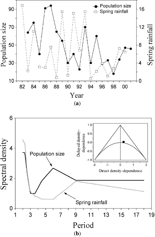
(a) Time-series of Purple Heron population dynamics (number of breeding pairs) and spring rainfall variability in the Albufera de Valencia, Eastern Spain, during a 20-year period. The declining trend of population size through time was subtracted with a cubic polynomial [71]. (b) Spectral densities of the time-series in (a) as a function of period; a Hamming window was used to smooth the spectral curve [71]. The inner graph in the upper right part of (b) shows the dynamics of the autoregressive model in the parameter space [8]; outside the triangle, populations tend to extinction, and below the parabola multiannual cycles arise; within the area between the triangle and the parabola populations exhibit dampened stability (on the right) or two-years cycles (on the left). The solid square denote de position of the Purple Heron time-series in the parameter space.
The Purple Heron is a large predatory waterbird, wintering in Tropical West Africa and breeding throughout Europe. Several authors have shown that the breeding numbers of Purple Herons in the Netherlands [58,59] and France [60] are strongly dependent on the weather conditions of the wintering area. Here, it will also be hypothesised that the population growth rate is a function of both local rainfall during breeding and current population size; the data for local rainfall comes from a meteorological station near the study area (P. Almaraz et al., unpublished work). Information on weather conditions of the wintering area can be furthermore included in the model. Previous analyses (P. Almaraz et al., unpublished work) suggested that 1-year lagged spring rainfall is the primary local climatic driver of interannual rate of change in breeding numbers; moreover, 1-year lagged summer ENSO and NAO indexes (see [11,13] for sources), correlated with local spring rainfall. The path diagram [33] depicting this hypothesised relationship is shown in Fig. 1b.
A preliminary analysis with an AR model [3,8] (Fig. 2b) suggests that the studied population is in the dynamic boundary between stability and multiannual cycles (dampened stability; [8]). However, within the framework of difference equations (AR models; [8]), it would be very difficult to include the indirect effects of rainfall on growth rate through population size, that is, to account for nonadditive effects of climate. Nevertheless, within the framework of SEM, this problem is largely circumvent. First, be the population size (breeding pairs) at time t, let be , and let stand for population growth rate. Be spring rainfall (Fig. 2a) and be a set of IID (identical and independently distributed) random variables. Finally, let and stand for the NAO and ENSO indexes, respectively. Assuming a Gompertz (log-linear) autoregressive model of first order ([8]; see Fig. 2b), and allowing for the covariation between large-scale climatic phenomena, the set of equations suggested by the verbal hypothesis proposed (Fig. 1b) can be written as:
| (5) |
| (6) |
| (7) |
| (8) |
In Eqs. (5) to (8) , and , are free parameters to be estimated from the observed variance–covariance matrix (). Note, however, that parameters , and μ are intercept terms; although they are easily implemented in SEM (e.g., [8, p. 129]), it will not be estimated here for simplicity (see also [26]). At this stage, we must construct measurement equations relating the true observations to the observations made during each survey, by means of detectability functions [26,61]. Let be the true log-population size at time t, and let be the log-detectability of ; if we let be the observation errors of the log-transformed counts, we get [27]:
| (9) |
Unfortunately, there is no information available on the observation error for in Fig. 1a. Nevertheless, since breeding Purple Herons are easily detectable during terrestrial visual counts, a of detectability can be safely assumed throughout the sampling period. Thus, for each survey in the raw data, 100 simulated counts were randomly subtracted from a normal variable with mean and coefficient of variation 0.3. The mean ± standard error of each count in the time-series was then recalculated from the simulated values, and the error variance of the observation errors (see below) was estimated from a linear regression between the standard deviations and the means on the log scale ([26]; the correlation between the real and simulated counts was, however, very high: , , ; see also [27]). (For simplicity, no sampling error will be assumed for rainfall values; note, however, that the procedure to implement them in the model would be the same.)
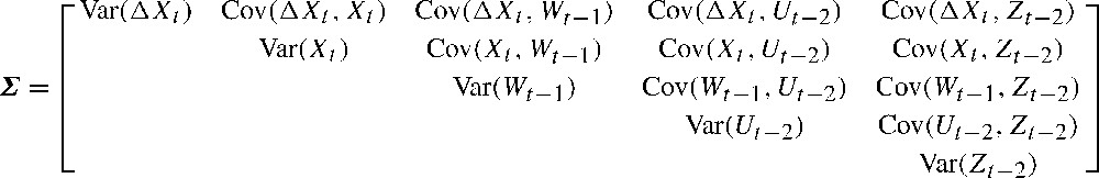
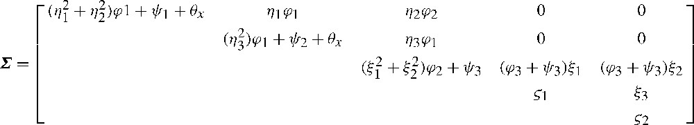
In order to estimate the biological parameters in Eqs. (5) to (8), a set of distributional assumptions regarding the model must be made [26,27]. For convenience, I will follow Refs. [24,26,31] in the notation. (1) Both log-transformed population size (), and rainfall were assumed to be drawn from time-invariant, normal distributions with means and constant variances ; that is, and . (2) The inter-annual stochastic variability impacting on each endogenous variable is assumed to describe a white noise process with 0 mean and constant variance ; that is, . (3) The observation errors, , are unbiased, independent, and additive on the log scale [24,26]; the error variances are denoted by , so . (4) Finally, NAO and ENSO proxy indexes were drawn from time-invariant, normal distributions with means and , and constant variances and , respectively; that is, , . Considering that both of them were measured without noise, and collecting variances across terms, matrix can now be rewritten as shown in Fig. 4.
A cautionary note should be made. Given that some variables (e.g., ) will have highly skewed distributions, the assumed wishart distribution of the observed matrix, , will probably not hold in general ecological settings. Thus, unknown parameters in were estimated with both ML and GLS methods, and associated uncertainties were assessed with the nonparametric bias-corrected bootstrap method (BCCI; [27,62]). All the analyses performed below were conducted in the SEPATH module of STATISTICA 6.1 [63,64].
The observed variance–covariance matrix shows evidence of departure from multivariate normality (Mardia-based Kappa=−0.201; [64]). Indeed, bootstrap resampling of the ML statistic shows a wide range of variation relative to the distribution of the GLS statistic (coefficient of variation, CV and 31%, respectively; log-variance ratio, , ; see Fig. 5). Additionally, the ML statistic (5.504, , d.f. = 4) had a 90% BCCI of 1.092–10.927, which corresponds to a range of P-values of (0.896–0.027). On the other hand, the GLS statistic (3.895, , d.f. = 4) had a 90% BCCI of (1.416–5.853), and a range of P-values of (0.841–0.210). Therefore, the bootstrap GLS method, which is robust against slight departures from normal kurtosis [31], suggests that the structural model proposed in Fig. 1b is consistent with the theoretical model expected given the data. On the other hand, the ML statistic shows a wide range of variability, and bootstrap resampling suggest that the observed model might not be consistent with the expected model.
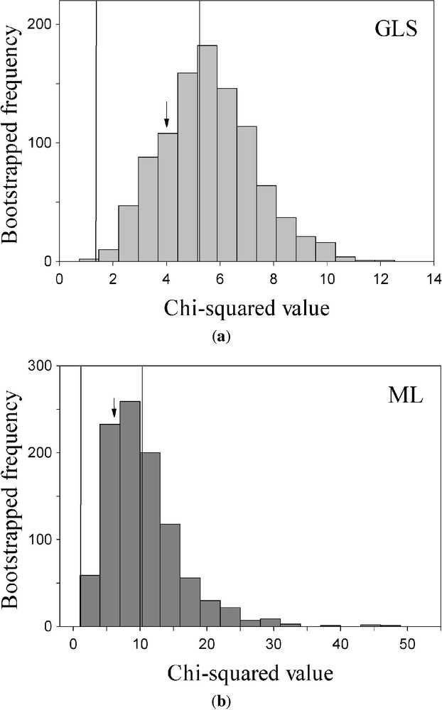
Frequency distributions of the bootstrapped set of Maximum Likelihood (ML, in (a) and Generalised Least-Squares (GLS, in (b) goodness-of-fit statistics of the model suggested by Fig. 1b. The arrow denote the point estimate of the statistic, and the vertical dotted lines depict de 90% bias-corrected bootstrap confidence interval. Note the different scaling of the x-axis.
Table 1 shows the bootstrap-GLS parameter estimates and associated uncertainties. As can be seen, the error variance () tended to underestimate density-dependence () and the climatic effect (; Table 3) relative to the simulated value (Table 1a); on the other hand, decreasing increased the magnitude of both parameters (Table 2). This result is consistent with the findings of Fromentin et al. [26] with the Norwegian Cod along the Skagerrak coast. In any case, bootstrapped uncertainty was, in general, a 30% larger than normal theory values across nearly all parameters (not shown). Altogether, results suggest that the effect of rainfall on growth rate operates both directly () and indirectly through population size () in this population, thus providing evidence for nonadditive effects of climate on growth rate [11,27]. Additionally, the large-scale climatic effects on local weather are not negligible, and the model further suggest that both oscillators were indeed teleconnected during the study period. Although for reasons of space they are not shown, performing the analysis with nested models [33] yielded identical results, and suggests similar parsimony and fit accuracy among models.
Parameter estimates and 90% bias-corrected bootstrap confidence interval (BCCI) for density dependence (), rainfall effect on growth rate (), rainfall effect on population size (), NAO effect on rainfall (), ENSO effect on rainfall (), and NAO-ENSO teleconnection (), assuming an error variance () of 0.22
| Parameter | Estimate | BCCI | BCCI |
| −0.366 | −0.523 | 0.080 | |
| 0.460 | 0.010 | 0.704 | |
| −0.328 | −0.505 | 0.114 | |
| 0.334 | −0.167 | 0.774 | |
| 0.356 | −0.286 | 0.782 | |
| 0.591 | 0.005 | 0.810 |
Same as Table 1, but assuming a 50% of higher variance in
| Parameter | Estimate | BCCI | BCCI |
| −0.144 | −0.356 | 0.125 | |
| 0.460 | 0.010 | 0.704 | |
| −0.129 | −0.505 | 0.114 | |
| 0.334 | −0.167 | 0.774 | |
| 0.356 | −0.286 | 0.782 | |
| 0.591 | 0.005 | 0.810 |
Same as Table 1, but assuming a 50% of lower variance in
| Parameter | Estimate | BCCI | BCCI |
| −0.433 | −0.654 | 0.075 | |
| 0.460 | 0.010 | 0.704 | |
| −0.470 | −0.692 | 0.131 | |
| 0.334 | −0.167 | 0.774 | |
| 0.356 | −0.286 | 0.782 | |
| 0.591 | 0.005 | 0.810 |
4.2 Fitting accuracy and time-series length: a Monte Carlo simulation
Since the statistical properties of both GLS and ML methods are asymptotic [31], it would be interesting to investigate the behaviour of several fit indexes with increasing time-series length. Therefore, an empirical Monte Carlo simulation was conducted at several time-series lengths [63,64] using the data and the SEM model for the Purple Heron dynamics. For each simulated length (, where years), 100 random SEMs were subtracted from the multivariate distribution of the covariance structure suggested by Fig. 1b; during each simulation, two measures of fitting accuracy were assessed: the scaled Akaike Information Criterion (AIC [55]) and the Brown–Cudeck Cross-Validation Index (CVI [31]). The smaller the value of both, the larger the fitting accuracy of the model tested [31]. Two sets of simulations were conducted, one with a GLS estimation of parameters and fit indexes, and the other with a ML estimation; the same random seed was specified at each simulation, so that the same sequence of random values were generated at each replication. This guaranteed that the only difference among the two sets of simulations was the parameter estimation method [63].
Results of the simulation (Fig. 6) suggest that both the AIC and the CVI decline sharply with increasing time-series length, an expected result given that both indexes are explicit functions of sample size. However, the simulated variance of both indexes with short time-series (N; Fig. 6) was higher in the ML method than in the GLS method (log-variance ratio, AIC: , ; CVI: , ); in spite of this, the mean value of the fit indexes were roughly similar across methods, and both their mean and variance converged with increasing length of the time-series. Thus, simulation results suggest that the fitting accuracy of GLS methods might be more robust against sampling variability at low sample sizes relative to ML methods. This results adds to previous findings [52] suggesting a larger statistical power of GLS, relative to ML, at low sample sizes in SEMs with equal number of free parameters. Overall, since ecological time-series are usually short, noisy, and nonlinear [7,19,22,23], with lengths of less than 50 years in most cases [65], GLS methods should thus be preliminarily considered as more robust alternatives to ML ([27,28]; see also [52] for an extensive review of the sociological literature).
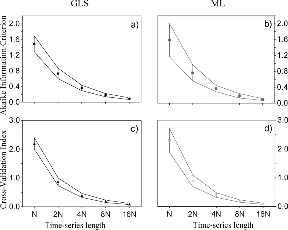
Behaviour of the scaled Akaike Information Criterion (a), (b) and the Brown–Cudeck Cross-Validation Index (c), (d) with increasing time-series length (dN, where N=18 years). Shown are mean values (symbols) and 95% confidence Intervals (vertical lines) of 100 Monte Carlo simulations performed with the covariance structure suggested by Fig. 1b at each time-series length, using both Generalised Least-Squares (GLS, in black) and Maximum Likelihood methods (ML, in grey).
4.3 The behaviour of alternative modelling approaches
As stated in the Introduction section, most of the ecological time-series modelling efforts make use of unstructured, simple autoregressive models to derive parameter estimates and conduct ecological inference (see, e.g., [7,9,11,16,22,66]). In this section such a model is constructed for the Purple Heron through Generalized Linear Modelling (GLZ; [27,64]), in order to compare the relative statistical performance between the SEM approach and the unstructured scheme. This model would take the topological form shown in Fig. 1a, which can be written as:
| (10) |
Table 4 shows the results of the fitting of Eq. (10) to the dataset. Besides the saturated model, all the possible nested models are shown. Although according to the Akaike Information Criterion (AIC) the model including joint density-dependent, rainfall and NAO effects was selected, dropping the NAO parameter from this model resulted in just a slight increase of the AIC (). Therefore, the final, most parsimonious model selected included only density-dependent and rainfall effects ( in Table 4). The difference in the AIC between this model and the full model (Eq. (10) and Fig. 1a; denoted by in Table 4) was of 1.398. Additionally, the magnitude of point estimates for parameters and even increased in model relative to model (Table 5). Thus, a full GLZ model including both intrinsic and multi-scale climatic effects, did not improve the statistical performance of the simplest case of no large-scale climatic effect, even though the SEM approach presented in this paper suggest indeed that a full model including a topologically complex structure (Fig. 1b) provides a highly plausible description of reality (see Section 4.1). This result is identical to that obtained in Ref. [27] with data from the Spanish population of White-headed Duck (Oxyura leucocephala), and is due to both the downscaled nature of the climatic dynamic effects and to the nonadditive effect of climate on growth rate through population density (see [27]).
Results of the fitting of the GLZ to the Purple Heron dataset. Each model is indicated by , where [⋅] contains the parameters included within each model tested (density-dependence; rainfall effect; NAO effect; ENSO effect). All the possible models within the full one are shown and ordered according to the Akaike Information Criterion (AIC). The Likelihood-Ratio test (L-R ) with associated p-value is also shown for each model. The model selected is shown on bold type
| Model | AIC | L-R | p-value |
| 35.434 | 22.613 | 0.000049 | |
| 35.796 | 20.257 | 0.000040 | |
| 36.175 | 19.878 | 0.000048 | |
| 37.194 | 22.858 | 0.000135 | |
| 37.446 | 16.607 | 0.000046 | |
| 37.739 | 20.314 | 0.000146 | |
| 38.173 | 19.879 | 0.000180 | |
| 38.666 | 17.386 | 0.000168 | |
| 41.518 | 14.534 | 0.000698 | |
| 43.502 | 14.550 | 0.002244 | |
| 44.778 | 9.275 | 0.002323 | |
| 44.912 | 9.141 | 0.002499 | |
| 45.810 | 10.242 | 0.005967 | |
| 46.460 | 9.592 | 0.008259 | |
| 49.251 | 4.801 | 0.028427 |
Parameter estimates for the full model () and the best one selected by the AIC () within the GLZ modelling of the Purple Heron data. Point estimate and associated standard error (S.E.) is shown for each parameter estimate along with the Wald statistic and associated p-value
| Model and parameters | Estimate | S.E. | Wald statistic | p-value |
| ENSO () | −0.085 | 0.170 | 0.247 | 0.619 |
| NAO () | 0.279 | 0.169 | 2.732 | 0.098 |
| Rainfall () | 0.284 | 0.158 | 3.239 | 0.072 |
| Population density () | −0.518 | 0.160 | 10.557 | 0.001 |
| Rainfall () | 0.316 | 0.157 | 4.046 | 0.044 |
| Population density () | −0.612 | 0.157 | 15.130 | 0.0001 |
Note, however, that according to the likelihood-ratio test the statistical fitting of all the possible GLZ models was relatively good albeit variable (Table 4).
5 Discussion
5.1 Advantages over traditional techniques
At the present, a wealth of studies provide strong evidence that both exogenous and endogenous forces are important in driving the dynamics of a population [7,11], and two major developments can be highlighted. First, some studies suggest that climatic variability can interact nonadditively with growth rate by modifying the population size at equilibrium [4,5,8,66] and by modifying population density directly [27]. Second, it is currently recognized that stochastic noise (whether environmental or demographic) and sampling error may play a major role in the dynamics of natural populations and in model assessment, respectively [3–5,7,9,11], and several methods have been proposed to assess their effects on population dynamics models (e.g., [6,22,23]). Nevertheless, incorporating nonadditive effects of climate in population models has prove difficult (but see [11]), and assessing the effects of noise sometimes requires extensive simulation and complex assumptions [7].
The technique outlined here provide several advantages in the light of these recent developments. For instance, given that a SEM is the combination of a measurement model and a structural model, it shares some conceptual issues with the Kalman filter and related state-based time-series analysis methods (see [6,22,23] for ecological examples). Indeed, by retaining the full observational model and specifying flexible priors a robust Bayesian approach can be easily implemented in a structural model with latent variables [43]. Additionally, complex but realistic assumptions regarding the measurement model can be made, for instance, to correlate perturbations across indicator variables [31]; this might be desirable in cases involving several orders in the density-dependent structure (e.g., see [26]). Furthermore, since both direct and delayed statistical density-dependence might be overestimated in the presence of autocorrelations in the error terms and/or an exogenous variable [18–20], a term for such autocorrelations can be furthermore included in the model (see [31] for details). Altogether, SEM allows all this information to be accounted for simultaneously in a complex and hierarchically structured network of endogenous/exogenous effects, as shown in Fig. 1b. Additionally, the multigroup SEM methodology [33] can be further extended to study the possible phase dependent nature of both the density dependent and the causal structure (P. Almaraz et al., unpublished work).
5.2 The issue of model selection
As noted by Stenseth et al. [13] including local climatic variables instead of large-scale climatic indexes in a population model, would add a problem of model selection, since several lags should be searched in order to find the best structure. Nevertheless, as stated in Section 2.3, biological populations respond only to the immediate climate, and the downscaling from large-scale climatic patterns to population parameters through local weather can yield divergent and unexpected results even within small geographic areas (see [12] for an example). Additionally, the presence of correlation between large-scale climate indexes and local weather variables can hinder some modelling efforts when using unstructured models (see [67] for a recent example). Thus, model selection with SEM must be a two-steps issue. First, one must conduct a “local-scale” analysis, in which the main local weather parameters driving the dynamics observed must be selected; once they are found, an “up-scaling” analysis must be aimed at relating those local weather parameters to large-scale climatic indexes. Through this procedure (applied in the example of Section 4), problems of model selection with climate variables (which are essentially a problem of spatio-temporal scale) are largely circumvent with SEM.
5.3 Model-data vs. model-reality consistency
One of the main advantages of SEM (namely, the specification of the covariance structure expected given a causal structure) can yet turn to be a dangerous feature during model assessment. Indeed, it should never be forgotten that the issue of whether the model is consistent with the data is different from the issue of whether the model is consistent with reality [31,38]. For instance, an exploratory approach conducted using some kind of discovery algorithm [38,51] can help in finding a set of models consistent with the data, given a rejection level. Fig. 7 depicts an example of this philosophy applied to the covariance structure studied in Section 4; as can be seen, both the theoretical topological complexity of the causal graph and the ability of the algorithm to resolve the direction of causality increases with the rejection level; thus, at very high levels (e.g., in Fig. 7) some impossible causal relationships may arise (for instance, a causal effect of population size at time t on the NAO index two years before). Note, however, that this is not a caveat of the discovery algorithm (upon which some restrictions can be imposed; see also [33,51]), but just the consequence of the algorithm being “blind” to the real nature of the variables although not to their statistical properties. Thus, a solid natural history and ecological knowledge of the study system (model-reality consistency) should always be confronted to a sound and robust statistical assessment of our model (model-data consistency), and vice versa. The issue to be learned from this example is best illustrated by Bollen's [31, p. 68] quote: “If a model is consistent with reality, then the data should be consistent with the model. But, if the data are consistent with a model, this does not imply that the model corresponds to reality.”
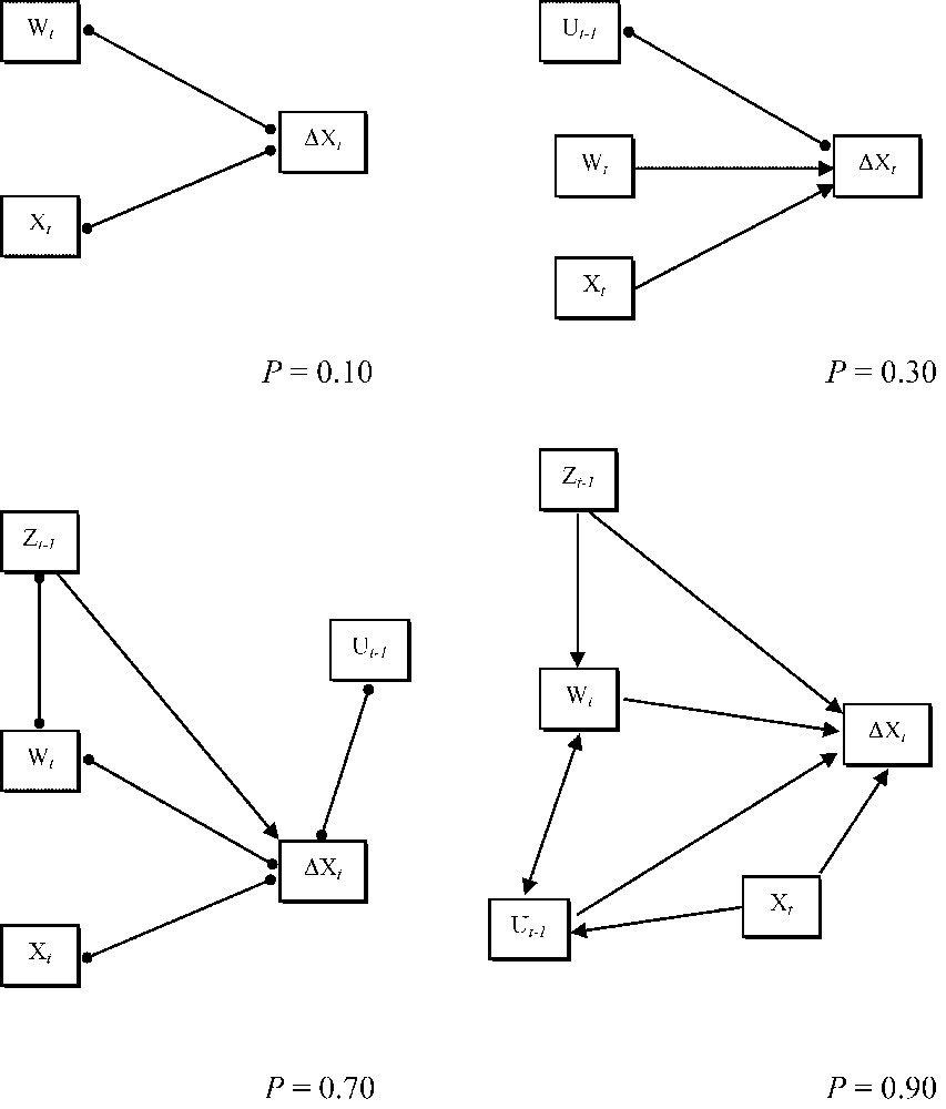
Several examples of partially directed inducing path graphs [33] obtained for the Purple Heron population dynamics. Each graph was obtained at a specific rejection level (denoted with P) with the SRS discovery algorithm [33,38,39], using the Method 2 of the program EPA2, provided in Ref. [33]. Double headed lines with solid dots represent unresolved causal relationships. Symbols for variables as in Fig. 1.
6 Conclusions, limitations and future prospects
Throughout this paper, I have commented on some important concepts and methods underpinning structural modelling with latent constructs techniques, and further provided an ecological example to demonstrate the potential of this technique when applied to time-series analysis in population ecology. In the light of currents debates on the nature, causes, and consequences of regulation for natural populations, SEM might stand out to be a key analysis tool for untangling complex multivariate relationships between climatic phenomena and population parameters. Indeed, the main advantage gained through the application of SEM to ecological time-series analysis is that complex biological assumptions take the form of a simple falsifiable empirical covariance structure that can be compared with a theoretical model to test for statistical consistence; that is, SEM goes beyond parameter estimation to provide statistical criteria on the plausibility of our initial hypotheses, and further provide tools to compare among alternative models with data as arbitrator. In this respect, SEM can be framed within the Lakatosian view of scientific development [68,69].
Finally, some current limitations of the SEM approach deserving further study must be outlined. First, although many relationships between climatic phenomena [13], ecological variables [7], and even between climatic and ecological variables [70] are highly nonlinear, SEM is, to date, largely limited to univariate linear relationships (but see [52]). The strategy of many modelling approaches in evolutionary ecology is to include quadratic terms in the univariate relationships to solve for nonlinearity, in the case of, e.g., disruptive selection (see review in [35,36]). However, quadratic and monotonic relationships might not be adequate in some highly nonlinear relationships [70], which are usually solved through generalized additive models including extra parameters. This problem is closely related to the second: the statistical performance of multiparameterized SEMs involving small sample sizes and noisy data has prove poor (e.g, [31,33]; see Section 4.1). For instance, the use of ADF estimation techniques is recommended only when sample size is greater than 1000, and both GLS and ML techniques reach their asymptotic properties when sample sizes are greater than 500 [52,54]. It is obvious that both figures are far beyond the longest population time-series available [65]. Additionally, a standard rule-of-thumb says that the number of data points (sample size) should be 6 times greater than the number of free parameters [31,33]. Thus, for instance, a model with 5 parameters, such as the one used in the above example, would require at least 30 years of data. The best of the solutions in this case would be to use Monte Carlo techniques to estimate parameters and the goodness-of-fit [53], which would also relax the distributional assumptions for the variables and the variance–covariance matrix.
Altogether, a major future development in ecological SEMs would be to provide state-based (Bayesian) versions of the standard frequentest approach [43]. The inclusion of nonlinear relationships, however, would not be as simple, since this would increase exponentially the number of parameters, the major statistical problem with ecological SEMs. However, all these are common problems to most statistical procedures, and, on the short term, only the availability of long time-series with low sampling variability [5,7,20] would provide ecological SEMs with the strong inferential power achieved in other scientific disciplines.
Acknowledgments
The ideas presented in the manuscript benefited from discussions with J.A. Amat, J. Bascompte, J.M. Gómez, N.C. Stenseth, and many people at the Alcalá II International Conference of Mathematical Ecology (AICME II). Three anonymous referees provided valuable comments. Research partially supported by a Sociedad Española de Ornitología/BirdLife International research grant.