

1 Introduction
Phytoplankton is a generic name for photosynthesizing microscopic organisms that inhabit the upper sunlit layer (euphotic zone) of almost all oceans and bodies of freshwater. They are agents for ‘primary production’ and the incorporation of carbon from the environment into living organisms, a process that sustains the aquatic food web [1].
More recent work has demonstrated the existence and potential importance of the formation of larger phytoplankton particles by aggregation [2–4]. However, the mechanisms governing aggregate formation have been poorly understood.
There has been extensive application of coagulation theory to describe aggregation of marine particles [5] and specifically phytoplankton aggregation [6,7]. Aggregation by physical coagulation requires that primary particles collide by some physical processes and stick together upon collision. Brownian motion, differences in sinking velocities and fluid shear may all cause primary particles to collide.
However, studies of marine aggregates at small scales have emphasized the biological mechanisms of their formation. That is, although planktonic organisms can be thought of as particles, the richness of biological responses makes the nature of their interactions more complex than the simple physical ones described by coagulation theory. Indeed, some planktonic species (algae, bacteria and dinoflagellates that are motile species of phytoplankton) have chemosensory abilities [8–10], that is, they can sense the chemical field generated by the presence of other cells. The dinoflagellates and more generally motile algae are known to leak organic matter such as amino-acids and sugar into solution [11] and this leakage creates zones around individual cells called ‘phycospheres’, where extracellular products exist in enhanced concentrations over the background [12]. The chemosensory responses allow dinoflagellates and algae that are present in a suitable neighborhood to find the leaky cells and to stay near them, forming aggregates. There has been no quantitative study of the nature of chemosensory interactions between dinoflagellates, even although chemosensory behavior in dinoflagellates may have importance in their search for food and for chemical defense [8–10,13–15]. Indeed, recent studies of micro-organisms have revealed diverse complex social behavior in dinoflagellates, such as cooperation in foraging and defense [9,16,17]. For instance, Pfiesteria dinoflagellates act as ambush predators, synchronously releasing toxins to kill all fish over many square kilometres, after which the dinoflagellates feed on the carcasses. On an other hand, many studies suggest that there will be a density at which dinoflagellates matabolites (for instance, an altruist production of toxins DMS (dimethyl sulfide)) will inhibit grazing and provide a protective feedback loop.
Based on the ideas of small scale biological mechanisms for aggregates formation, El Saadi and Arino [18,19] have investigated a Lagrangian model which provides an explanation of the aggregation behavior in phytoplankton in terms of attraction mechanisms among cells due to the chemosensory behavior, random branching (birth and death), in addition to individual random dispersals described by independent Brownian motions. The aim of such modelling was to catch the main features of the individual dynamics at small scales which are responsible at a larger scale for a more complex behavior that leads to the formation of aggregating patterns. An Eulerian description has been rigorously derived as a continuum limit [18,19] by using the approach in [20] based on martingale properties of a sequence of approximating interacting branching-diffusion processes. The Eulerian model of phytoplankton aggregation is described by the following nonlinear stochastic partial differential equation defined in space of vector measures:
| (1) |
In [25], it has been shown that if the branching phenomenon is not present in the phytoplankton story, (for every ) is absolutely continuous with respect to the Lebesgue measure on , and hence, admits a density which satisfies the integro-differential advection–diffusion equation:
| (2) |
This paper is a contribution in exploring phytoplankton aggregation behaviors using an IBM approach. The IBM's models have known an important development in the 1990s stimulated by the availability of powerful personal computers [26–28]. The article written by Huston et al. [29] is the most frequently quoted. These authors argue that the development of this approach is due to the need to take into account the individual because of his genetic uniqueness and, secondly, the fact that each individual is situated and his interactions are local. We recall that the principle of an IBM consists in following each individual of a collection, assuming they move or some of their characteristics change during a time step, due to a number of influences such as individual behavior, interactions of individuals with one another, interactions of individuals with a resource distribution [30]. So in this work, we propose to build a numerical IBM (Individual-Based Model) version arising from the Lagrangian model of phytoplankton in [18,19] and present the simulations results showing the behavior of the system of stochastic differential equations in [18,19]. Our goal is twofold: first, to visualize the formation of clusters, and second, to measure and compare influences of the different processes involved at the cell level on appearing of aggregation patterns.
The paper is organized as follows: in Section 2, we describe the Lagrangian aggregation model of phytoplankton built in [18,19]. Section 3 is devoted to the simulator description and in Section 4, we present the different scenarios to be tested. Section 5 summarizes the simulations results. These correspond to the following issues: (1) the Clark–Evans Index; (2) the spatial and temporal distribution of phytoplankton cells; (3) the effect of diffusion; and (4) the effect of perception. Section 5 offers a discussion of the results and finally, we give some conclusions in Section 6.
2 Lagrangian aggregation model
We recall that the Lagrangian model of phytoplankton aggregation in [18,19] is built up as follows:
2.1 Spatial motion
We consider N phytoplankton cells (N is a positive integer), each of them having at some time a certain position. Let be the family of positions for the N cells.
The spatial motion of phytoplankton cells is described via the following system of stochastic differential equations:
| (3) |
2.2 Spatial interactions
To describe interactions between phytoplankton particles, we propose the ideas involving non-uniformity of the concentration fields around organisms and consider phytoplankton cells having chemosensory abilities (dinoflagellates, algae) and hence some knowledge about their neighbors. However, each cell has a limited knowledge of the spatial distribution of its neighbors because it cannot detect small concentration differences over its length [31,33,34].
Taking into account these biological considerations, we assume that aggregation forces act over a specific range of sensitivity and thus we model pair interactions as follows:
- – The presence of a cell in position y induces on a cell in position x an attractive force that depends on the distance between the two cells and which is determined by:
where(4)
( and are the non negative reals that delimit the range of sensitivity in phytoplankton).(5) The normalization factor in (4) corresponds to associating the mass to each phytoplankton cell [23,35]. leads to the attraction of the cell in position x to that in y. The quantity gives the magnitude of as a function of the distance . The direction of is given by the unitary director vector . The cell in position x is not attracted to that in y if , because in the closest vicinity of y is the largest concentration of the substances released by the cell in y. It has been reported that large concentrations of products such as amino acids, organic compounds and sugar inhibit the chemosensory behavior in dinoflagellates and motile algae [8];
- – The drift is the superposition of all cells effects of the system on the ith cell. It is given by:
2.3 Branching
The cells branch. The most common mean of reproduction in phytoplankton is asexual cell division (mitosis). This process splits the organism into two identical copies. So, we assume that each cell can die, divide into two or remain unchanged with equal probabilities. If the phytoplankton cell splits, the two new cells begin their life at the branching point. They move following Eq. (3) until the time they themselves branch and so on. A cell division can occur once every day.
3 The simulator
We now present the IBM arising from the Lagrangian model introduced in the previous section, that is its computer simulation model.
The simulator we conceived is a tool of experiments intended to represent virtually individual aggregating behavior. It is implemented in the object-oriented language Smalltalk using the Visual Works Environment. The model of this simulator is based on the discrete version of the system of stochastic differential equations (3) with K replaced by (4). Time evolves in a discrete way by steps Δt. The initial condition is prepared by placing randomly and independently N particles. Each time step consists of two stages: (1) branching (random birth and death); (2) spatial motion. At the first stage, each particle splits into two or dies or remains unchanged with equal probabilities. If it splits, the new particle is placed on top of the parent; if it dies, it is removed from the system. In stage 2, the ith particle is displaced to a new position:
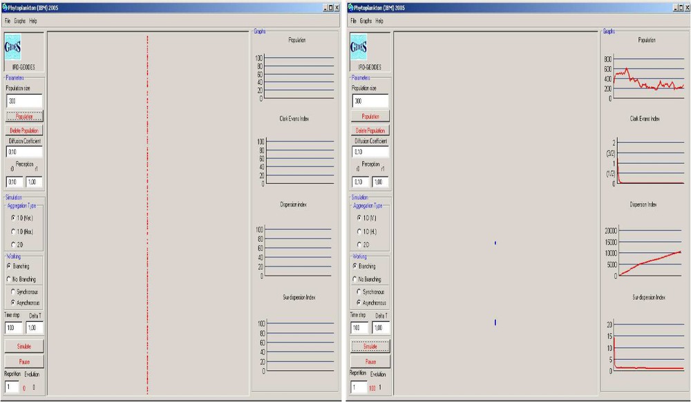
The simulator is provided with an interface to perform action-to-visualize the aggregation behavior (Fig. 1). It consists on three components:

The interface of the simulator.
- (i) the parameter window (on the left) that allows the user the set up of the global variables;
- (ii) the situation window (at the center of the interface) that represents positions of individuals;
- (iii) the indicator window (on the right) that allows to visualize evolution of differents indicators of aggregation.
The simulator offers the possibility of visualizing the dynamics of phytoplankton cells in 1D (vertically or horizontally) and in 2D. It permits one to undertake simulations in two situations: the model including branching mechanisms (model I) and the model without branching (model II) (that is, the population size remains fixed). It has also been performed in order to quantify the evolution of different indicators of aggregation (Clark–Evans Index, the dispersion index and the surdispersion index) [36]. The last analyzes and characterizes the spatial structure of the particle pictures shown by the simulator.
For a purely qualitative aim, we present some particle pictures describing the reproduction and temporal-spatial spread of phytoplankton communities in 1D (Fig. 2) and 2D (Fig. 3).
A time-evolution result for the Lagrangian model in 1D.

A time-evolution result for the Lagrangian model in 2D.
In this work, we restrict ourselves to the 1D numerical results obtained by using the Clark–Evans Index defined as:
It has been shown (see [37]) that:
Our approach in using this indicator has a double goal: on the one hand, we intend to explore the spatial structure of the particle pictures stemmed from both model I and model II, and on the other hand, to measure and compare influences of the different processes in play (random dispersion, chemosensory interactions and branching) on the aggregating patterns.
4 Scenarios tested
The Lagrangian model in Section 2 gives an explanation of the phytoplankton aggregating behavior in terms of a diffusion with velocity D, attractive forces acting in a perception zone delimited by and and a branching with a fixed rate.
We are therefore going to explore several scenarios corresponding to different values of D and . The values of D are chosen to correspond at three different orders of magnitude that cover possible values of phytoplankton diffusion quoted in the literature. These values are (, , ). For , we consider different arbitrary possible values that are well suited to the choice of (, 10, 20 μm). We fixed an arbitrary value chosen very small in comparison to the values of () [30].
Although many preliminary experiments have shown no variability in the outputs, we perform five runs of the simulation for each scenario to damp out any randomness embodied in the simulator. Hence, each simulation result presented in the next section is an average of five repetitions. Furthermore, these preliminary experiments have also shown that for model II and for model I are sufficient long time to reach stable aggregative structures, with a time step . To connect these simulations with reality, we let Δt correspond to 1 day in reality, since a cell division holds once every day.
The nine scenarios summarized in Table 1 are explored in the two cases:
Table of scenarios
| 1 (μm2) | 10 (μm2) | 20 (μm2) | |
| S1 | S2 | S3 | |
| S4 | S5 | S6 | |
| S7 | S8 | S9 |
- (1) model I (the interacting branching model);
- (2) model II (the interacting model without branching).
5 Simulations results
We present the simulations results obtained for an initial population size , with a random initial distribution. A difference appears between results coming from models I and II. Moreover, in the case of model II, some differences due to the variation of the parameters D and are observed between the scenarios.
5.1 Result 1 (Clark–Evans Index)
A difference in the evolution of the Clark–Evans Index (CEI) between models I and II is shown in Figs. 4 and 5.

The CEI's evolution in time for model I.

The CEI's evolution in time for model II.
For model I, the CEI is close to 0 in all the scenarios, which indicates a strong aggregation. The values greater than 0 observed earlier the date s are due to the randomness of the initial distribution. In the case of model II, the CEI is greater than 0 in all the scenarios, which corresponds to a less good aggregating behavior. The best aggregation in this case is observed in scenario 2, while instability is observed in scenario 9.
5.2 Result 2 (spatial and temporal distribution)
Both of models I and II in Figs. 7 and 8 show clusters formation from a random initial distribution (Fig. 6). Not only in the figure of model II, the clusters have larger diameter and small sizes, but also the peaks of the density profile observed in the figure of model I are higher: the aggregation phenomenon is stronger in the case of an interacting model with branching.

The spatial distribution of model I at time T=100.

The spatial distribution of model II at time T=1000.

The initial spatial distribution.
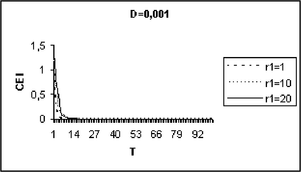
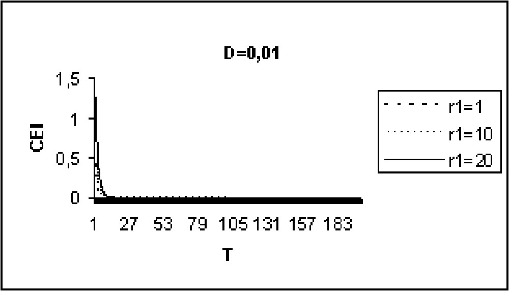
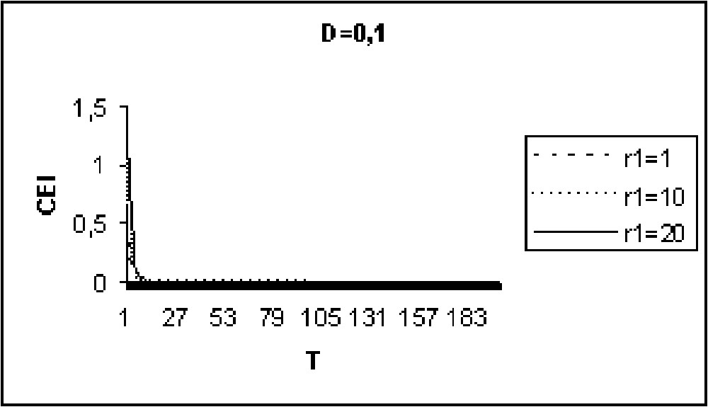
5.3 Result 3 (effect of diffusion)
Experiments in Figs. 9 to 11 show that for model I, the CEI is not affected by a variation of D. However, in the case of model II (Figs. 12 to 14), there are some differences in the evolution of the CEI. Aggregation is better for a weak diffusion coefficient and instability occurs for largest values of D.
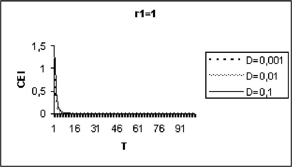
The CEI variation in time when (model I).

The CEI variation in time when (model I).
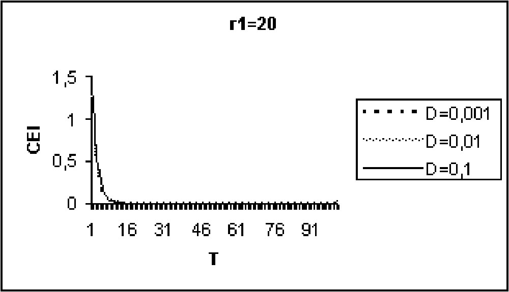
The CEI variation in time when (model I).

The CEI variation in time when (model II).

The CEI variation in time when (model II).
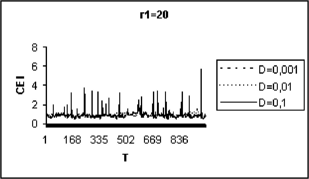
The CEI variation in time when (model II).
5.4 Result 4 (effect of the perception zone)
As shown in Figs. 15 to 17, the CEI is not affected by a variation of the perception radius length, in the case of model I. For model II (Figs. 18 to 20), differences are observed in the CEI evolution. The best aggregation is observed for and a great number of fluctuations appears at largest value of .
The CEI variation in time when D=0.001 (model I).
The CEI variation in time when D=0.01 (model I).
The CEI variation in time when D=0.1 (model I).

The CEI variation in time when D=0.001 (model II).

The CEI variation in time when D=0.01 (model II).
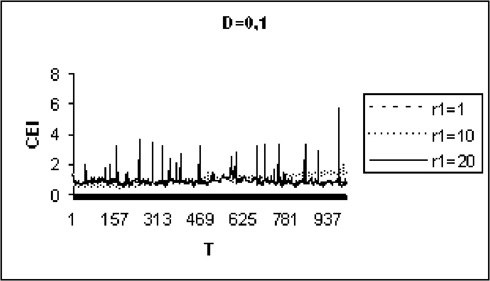
The CEI variation in time when D=0.1 (model II).
6 Discussion
All the simulations results presented earlier make obvious the aggregating phenomenon in phytoplankton. Indeed, the CEI is always less than 1 in both of models I and II, that is, clusters do not form only when particles (phytoplankton cells) diffuse, interact spatially and branch, but even when the branching process is ignored. This last result confirms our asymptotic analytic result in [25] on the emergence of aggregating patterns at large scale from a particle system with nonlinear interactions at small scales.
However, a difference is noticed between the interacting model with branching and that without branching. Aggregation is stronger and more visible when branching mechanisms are taken into account. From a biological view, this is due to the spatial aspects coupled to the branching mechanism. Indeed, there is a fundamental difference between the locations of birth and death: deaths occur anywhere but births always occur adjacent to living organisms. The accumulation of these small-scale density fluctuations produce the palpable nonuniformities detected in Figs. 2 and 3.
Diffusion and sensory distances have both a role on the aggregating behavior but this role remains negligible comparatively to the branching effect. It is clear this is due to the small values of the diffusion coefficient for phytoplankton and to the different lengths of the perception radius chosen for . Some simulations (which we do not present here) show that greater values of D and (for example, D beyond 5 and beyond 30) lead to particle pictures very different of those presented in this paper. Effects of the diffusion and/or the sensory distance on the quality of the aggregation behavior are better observed when branching mechanisms are ignored. In the latter, simulations show a transition from a random distribution to an organized structure with formation of weak clusters characterized by their larger radius and lower sizes, in contrast with the clusters occurring when branching; and the best situation for aggregation in this case is when diffusion is weak and the radius of perception is average. Instability in the spatial structure often occurs for the interacting model without branching. We think that this observation can give some intuitive insight on the stability of the steady-state solution in [25].
7 Conclusions
In this paper, an IBM approach was undertaken in the study of the aggregation process in phytoplankton. We have conceived and simulated the IBM discrete version corresponding to the mathematical Eulerian model in [18,19]. Simulations results show the formation of clusters, qualitatively by visualizing the aggregation phenomenon and quantitatively by using an aggregation indicator: the Clark–Evans Index.
The main result of this work is that branching has an eminent role in the phytoplankton aggregation process. We point out that Young in his paper [38], has shown that a population of independent random-walking organisms, reproducing by binary division and dying at constant rates, aggregates and clusters form out of spatially homogeneous initial condition without environmental variability, kinesis or taxis. He stressed the fact that the clustering mechanism can be driven only by reproduction and death (branching), provided the diffusion is not too strong relative to the reproduction rate. Here in this work, we rediscover Young's result of [38,39], although our population is spatially dependent. Indeed, simulations results stemmed from our IBM model have shown the formation of very weak clusters when only diffusion and interactions are involved in the model, while the clustering mechanism becomes more important and visible when branching is taken into account. Consequently, the IBM approach presented in this paper, confirms that the mathematical Eulerian model (1) investigated in [18,19] is really an aggregation model and establishes the importance of branching on the aggregation phenomenon relative to nonlinear interactions and diffusion.
On another hand, many qualitative and quantitative results on the spatial distribution, sizes and positions of aggregates in space and time could be provided by our IBM model.
Acknowledgements
The authors would like to thank Professors Pierre Auger, Jean-Pierre Treuil, Christian Mullon, and Nicolas Bacaer for numerous useful discussions.