Elliptical Fourier descriptors for contours in three dimensions: A new tool for morphometrical analysis in biology

Jérémy E. Godefroy; Fabien Bornert; Catherine I. Gros; André Constantinesco

doi:10.1016/j.crvi.2011.12.004

Medical sciences/Sciences médicales

Elliptical Fourier descriptors for contours in three dimensions: A new tool for morphometrical analysis in biology
[Descripteurs elliptiques de Fourier des contours en trois dimensions: un nouvel outil pour l’analyse morphométrique en biologie]

Jérémy E. Godefroy ¹ ; Fabien Bornert ² ; Catherine I. Gros ² ; André Constantinesco ¹

¹ IMFS CNRS FRE 3240, Preclinical Imaging Lab, biophysique et médecine nucléaire, hôpitaux universitaires de Strasbourg, 1, avenue Molière, 67098 Strasbourg cedex, France
² Inserm UMR 977, faculté dentaire, hôpitaux universitaires de Strasbourg, 11, rue Humann, 67000 Strasbourg, France

Comptes Rendus. Biologies, Volume 335 (2012) no. 3, pp. 205-213.

Résumés

Anglais
Français

Elliptical Fourier descriptor analysis is a method for the morphometric study of curves. It has been used in the two-dimensional plane for closed contours, but rarely for lines in the three-dimensional space. The method consists of an expansion of a contour as a sum of ellipses. In this article, we study three-dimensional contours, i.e. lines embedded in the three-dimensional space. We compute for the first time the relations between the Fourier coefficients and its geometric parameters. We then use these relations for normalization and reorientation of three-dimensional contours. Such an algorithm can be used to perform inter-individual comparisons between contours, regardless of differences in viewpoint or global size. Human and small animal illustrative examples using biomedical X-ray CT imaging data of open bone structures demonstrate the interest and potential of the method for morphological analysis.

Les descripteurs elliptiques de Fourier permettent l’analyse morphométrique des courbes. Ils ont été essentiellement employés en biologie pour l’analyse de lignes fermées dans l’espace à deux dimensions mais rarement pour des lignes inscrites dans l’espace à trois dimensions. La méthode consiste en la décomposition d’un contour en somme d’ellipses, appelées « harmoniques elliptiques ». Dans cet article, nous étudions des contours inscrits dans l’espace à trois dimensions et déterminons, pour la première fois, les relations existant entre les coefficients elliptiques de Fourier et les paramètres géométriques correspondant. Ces relations sont alors utilisées pour la normalisation et la réorientation des contours tri-dimensionnels. L’algorithme est ainsi adapté à la comparaison inter-individu du contour d’une même structure, indépendamment des différences de dimensions ou de point de vue. Des exemples biologiques illustrant le potentiel de la méthode pour l’analyse morphométrique sont exposés à partir de données clinique et préclinique d’imagerie tomodensitométrique de structures osseuses ouvertes.

Métadonnées

Reçu le : 2011-06-24
Accepté le : 2011-12-18
Publié le : 2012-01-25

PMID

DOI : 10.1016/j.crvi.2011.12.004

Keywords: Elliptical Fourier descriptors, Morphology, Three-dimensionnal contours, Reorientation algorithm, Rescaling, Contour comparison
Mot clés : Descripteurs elliptiques de Fourier, Morphologie, Contours en trois dimensions, Algorithme de réorientation, Mise à l’échelle, Comparaison du contour

Affiliations des auteurs :

Jérémy E. Godefroy ¹ ; Fabien Bornert ² ; Catherine I. Gros ² ; André Constantinesco ¹

¹ IMFS CNRS FRE 3240, Preclinical Imaging Lab, biophysique et médecine nucléaire, hôpitaux universitaires de Strasbourg, 1, avenue Molière, 67098 Strasbourg cedex, France
² Inserm UMR 977, faculté dentaire, hôpitaux universitaires de Strasbourg, 11, rue Humann, 67000 Strasbourg, France

@article{CRBIOL_2012__335_3_205_0,
     author = {J\'er\'emy E. Godefroy and Fabien Bornert and Catherine I. Gros and Andr\'e Constantinesco},
     title = {Elliptical {Fourier} descriptors for contours in three dimensions: {A} new tool for morphometrical analysis in biology},
     journal = {Comptes Rendus. Biologies},
     pages = {205--213},
     publisher = {Elsevier},
     volume = {335},
     number = {3},
     year = {2012},
     doi = {10.1016/j.crvi.2011.12.004},
     language = {en},
}

TY  - JOUR
AU  - Jérémy E. Godefroy
AU  - Fabien Bornert
AU  - Catherine I. Gros
AU  - André Constantinesco
TI  - Elliptical Fourier descriptors for contours in three dimensions: A new tool for morphometrical analysis in biology
JO  - Comptes Rendus. Biologies
PY  - 2012
SP  - 205
EP  - 213
VL  - 335
IS  - 3
PB  - Elsevier
DO  - 10.1016/j.crvi.2011.12.004
LA  - en
ID  - CRBIOL_2012__335_3_205_0
ER  -

%0 Journal Article
%A Jérémy E. Godefroy
%A Fabien Bornert
%A Catherine I. Gros
%A André Constantinesco
%T Elliptical Fourier descriptors for contours in three dimensions: A new tool for morphometrical analysis in biology
%J Comptes Rendus. Biologies
%D 2012
%P 205-213
%V 335
%N 3
%I Elsevier
%R 10.1016/j.crvi.2011.12.004
%G en
%F CRBIOL_2012__335_3_205_0

Jérémy E. Godefroy; Fabien Bornert; Catherine I. Gros; André Constantinesco. Elliptical Fourier descriptors for contours in three dimensions: A new tool for morphometrical analysis in biology. Comptes Rendus. Biologies, Volume 335 (2012) no. 3, pp. 205-213. doi : 10.1016/j.crvi.2011.12.004. https://comptes-rendus.academie-sciences.fr/biologies/articles/10.1016/j.crvi.2011.12.004/

Version originale du texte intégral

1 Introduction

Elliptic Fourier descriptor analysis is a method for contour description. A closed curve is a continuous periodic function of a parameter, so it can be alternatively represented as a sum of cosine and sine functions of growing frequencies, affected by coefficients referred to as ‘Fourier descriptors’ (FDs). The sum of these cosine and sine functions converges towards the initial contour, as the number of harmonics increases. Each harmonic is actually an ellipse, completely defined by its period and its FDs.

Elliptical Fourier descriptors were first described in the two-dimensional space [1–4] with some variety regarding the variable used for parametrization (arc length, angle, etc.). A plane, closed contour is expressed as a sum of two-dimensional ellipses of decreasing areas. The FDs can be used as morphometric variables in multivariate analysis, allowing for the distinction of groups within a set of shapes. Most applications in two dimensions are related to biological issues [5], for anthropology [6–8], anatomy [9], evaluation of the response to orthodontics treatment [10], etc. Hand-written character recognition [2,11,12] or aircraft recognition algorithms [3,13] are other areas of use. The FDs allow for the computation of invariants of the contour, independent under translation, rotation or change in the starting point on the contour [2,4]. In addition to providing interesting information compression, FDs can be used for smoothing contours, by keeping only the first harmonics.

In three dimensions, two different problems may be addressed. One is the study of bounding surfaces [14–19] where shapes are described as sum of ellipsoids. The other is the study of closed lines embedded in the three-dimensional space. Few papers have been published on the subject. Numerical invariants of three-dimensional contours are computed in reference [20] to study the influence of noise and distortion for shape recognition purposes. In reference [21], lines are simplified as ‘chaincodes’, reducing the complexity of the initial contour. FDs are computed using this formalism, and normalized to make them independent of scale change and orientation of the global contour. In reference [22], the author makes the FDs independent of the starting point and uses them in the cardiology field to identify supraventricular beats by analyzing the 3D curves formed by the electrocardiogram vector (QRS loop). In reference [23], the authors used 3D FDs to optimize the fitting of protection harnesses to body shape. Some works make use of the results in two dimensions for studying surfaces, either by ‘slicing’ the initial 3D surface [24–26], by combining projections [27] or using invariants [28]. None of these papers give an explicit correspondance between FDs and their geometric parameters.

In this article, we study lines embedded in three-dimensional space. Real world objects, more particularly, anatomical structures, tend to be three-dimensional rather than two-dimensional. Tomographic imaging such as scanner and MRI, followed by appropriate image processing, may be used to create three-dimensional objects. We focused on lines rather than surfaces for several reasons. First, mathematical simplicity: Lines may be parametrized by one-variable functions while surfaces require the handling of multiple variable functions. Secondly, many anatomical structures (such as skull or heart) are not closed surfaces, making irrelevant the use of global surface descriptors in the vicinity of the boundary. Unlike reference [21], we did not restrict ourselves to chaincodes, but rather dealt with arbitrary 3D lines.

We start from two 3D lines. Each line represents a contour and has a set of coordinates (sampling) describing it. The aim of this article is to address the following question: how can we compare the two contours? When the sampling of the points on the contours is done in two different Cartesian coordinate systems, we cannot compare directly the lines but we need a transformation step. Our approach is to use the decomposition as elliptical Fourier descriptors to find, for each object, an intrinsic Cartesian coordinate system to perform this transformation. This system will be specific to each contour. As stated earlier, each harmonic of the decomposition of a contour is an ellipse defined by its period and FDs. The first harmonic is an ellipse roughly approximating the contour. We use it as the reference plane of the new Cartesian coordinate system, its symmetry axes being the two axis lines X, Y. We also use the area of this first harmonic to account for the potential scale difference in the two coordinate systems. Making ue of these results, we compute an algorithm for rescaling and reorientation of 3D objects, by normalizing their FDs or their coordinates on the first harmonic.

An ellipse can be described in two ways: either by giving the coefficients of its parametric equation (six numbers in three dimensions), or by giving the geometrical parameters: semi-axis lengths, angles for the orientation (three numbers in three dimensions), starting point on the contour and direction of motion when the parameter increases. In order to perform the normalization-reorientation steps described above, we must know the equations linking the geometrical parameters of a given ellipse (here, the first elliptical descriptor) to the coefficients of its parametric equation (the FDs of the first harmonic). This has been addressed by reference [3] in two dimensions, but not in three dimensions. This is the subject of the Section 2.

To introduce the formalism later used in this article, let us consider a closed curve M(t) of coordinates (x(t), y(t), z(t)). It can be described as a sum of ellipses using the Fourier series expansion of its coordinates:

x (t) = x_{0} + \sum_{n = 1}^{\infty} x_{n} (t)

with

x_{0} = \frac{1}{T} \int_{0}^{T} x (t) d t

where T is the period of x(t),and

x_{n} (t) = x_{c_{n}} \cos (2 n π t / T) + x_{s_{n}} \sin (2 n π t / T), n \in ℕ^{*}

with

x_{c_{n}} = \frac{2}{T} \int_{0}^{T} x (t) \cos (\frac{2 n π t}{T}) d t

x_{s_{n}} = \frac{2}{T} \int_{0}^{T} x (t) \sin (\frac{2 n π t}{T}) d t

x_{c_{n}}, x_{s_{n}}

are the Fourier coefficients of the n-th ellipse. The same relations hold true for y and z. For the experimental work, x(t) will typically be obtained by sampling a contour by p points x_m, m = 1,…, p. The direction of motion when the parameter t increases is the direction of sampling on the contour. The FD's computed here will depend on the point chosen to be x₁ and the direction of sampling on the contour.

So

\vec{O M (t)} = \vec{O C} + \vec{C M} = \vec{O C} + \sum_{n = 1}^{\infty} \vec{C M_{n} (t)}

where C (x₀,y₀, z₀) and

\vec{C M_{n} (t)}

(x_n(t), y_n(t), z_n(t)). M_n(t) describes an ellipse E_n centered at C. Let a, b be the lengths of its semi-axis, α, β, γ three angles that define its three-dimensional orientation, and φ the phase shift for t = 0. The purpose of the next section is to find the equations relating

x_{c_{n}}, x_{s_{n}}, y_{c_{n}}, y_{s_{n}}, z_{c_{n}}, z_{s_{n}}

and a, b, α, β, γ, and φ.

2 Relations between Fourier coefficients and geometrical parameters for ellipses in the three-dimensional space

To determine the relations between the coefficients (x_c, x_s, y_c, z_c, z_s) and the geometrical parameters a, b, α, β, γ, φ, we start from an ellipse in the two-dimensional plane, defined by its axes $(O, \vec{i})$ and $(O, \vec{j})$ , its period T, a phase shift φ (corresponding to the position of M at t = 0). Its parametric equation is given by:

(\begin{array}{c} x (t) \\ y (t) \\ z (t) \end{array}) = (\begin{array}{c} a \cos (2 π t / T + φ) \\ b \sin (2 π t / T + φ) \\ 0 \end{array})

Let us define now the rotation of this ellipse in the three-dimensional space for any given orientation. For this purpose, we use Euler angles α, β, γ, illustrated in Fig. 1. Any orientation can be achieved by composing three elemental rotations r_α, r_β, r_γ.

Figure 1
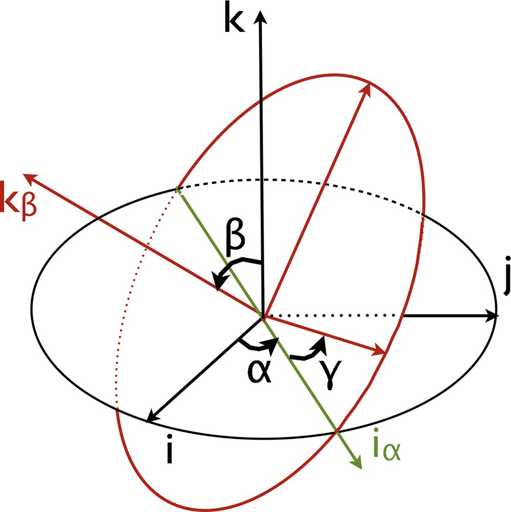
Illustration of the Euler angles used in this study.

Here, r_α is a rotation of angle α about the $(O, \vec{k})$ axis, whose matrix R_α is written in the basis $(\vec{i}, \vec{j}, \vec{k})$ ; r_β is a rotation of angle β about the $(O, {\vec{i}}_{α})$ axis, with ${\vec{i}}_{α} = r_{α} (\vec{i})$ , whose matrix is R_β; r_γ is a rotation of angle γ about the $(O, {\vec{k}}_{β})$ axis, with ${\vec{k}}_{β} = r_{β} (\vec{k})$ , whose matrix is R_γ.

The matrix Ω of this transformation ω, written in the basis $(\vec{i}, \vec{j}, \vec{k})$ , is:

Ω = R_{γ} R_{β} R_{α} = (\begin{array}{l} \cos α \cos γ - \sin α \cos β \sin γ & - \cos α \sin γ - \sin α \cos β \cos γ & \sin α \sin β \\ \sin α \cos γ + \cos α \cos β \sin γ & - \sin α \sin γ - \cos α \cos β \cos γ & - \cos α \sin β \\ \sin β \sin γ & \sin β \cos γ & \cos β \end{array})

The (Ω_ij)_{i, j = 1,…, 3} satisfy:

Ω_{11} Ω_{12} + Ω_{21} Ω_{22} + Ω_{31} Ω_{32} = 0

(1)

Ω_{11}^{2} + Ω_{21}^{2} + Ω_{31}^{2} = 1

(2)

Ω_{12}^{2} + Ω_{22}^{2} + Ω_{32}^{2} = 1

(3)

So any ellipse whose parametric equation is (X(t), Y(t), Z(t)), can be written as

(\begin{array}{c} X (t) \\ Y (t) \\ Z (t) \end{array}) = Ω (\begin{array}{c} x (t) \\ y (t) \\ z (t) \end{array}) = (\begin{array}{c} x_{c} \cos (2 π t / T) + x_{s} \sin (2 π t / T) \\ y_{c} \cos (2 π t / T) + y_{s} \sin (2 π t / T) \\ z_{c} \cos (2 π t / T) + z_{s} \sin (2 π t / T) \end{array})

The problem is equivalent to finding a, b, α, β, γ, φ, given x_c, x_s, y_c, y_s, z_c, z_s, bound by the following equations:

S x \{\begin{array}{l} x_{c} = & a Ω_{11} \cos φ + b Ω_{12} \sin φ \\ x_{s} = & - a Ω_{11} \sin φ + b Ω_{12} \cos φ \end{array},

and the same for S_y and S_z by replacing Ω_1i by Ω_2i and Ω_3i, respectively.

Using S_x, S_y and S_z in Eqs. (1) to (3), we get:

\tan 2 φ = 2 \frac{x_{c} x_{s} + y_{c} y_{s} + z_{c} z_{s}}{x_{s}^{2} + y_{s}^{2} + z_{s}^{2} - x_{c}^{2} - y_{c}^{2} - z_{c}^{2}}

(4)

a^{2} = (x_{c}^{2} + y_{c}^{2} + z_{c}^{2}) \cos^{2} φ + (x_{s}^{2} + y_{s}^{2} + z_{s}^{2}) \sin^{2} φ - (x_{c} x_{s} + y_{c} y_{s} + z_{c} z_{s}) \sin 2 φ

(5)

b^{2} = (x_{c}^{2} + y_{c}^{2} + z_{c}^{2}) \sin^{2} φ + (x_{s}^{2} + y_{s}^{2} + z_{s}^{2}) \cos^{2} φ + (x_{c} x_{s} + y_{c} y_{s} + z_{c} z_{s}) \sin 2 φ

(6)

Eq. (4) has four solutions φ₁,…,φ₄:

φ_{n} = φ_{0} + \frac{n π}{2}, n \in \{0,1,2,3\} with φ_{0} = (1 / 2) \arctan \frac{2 (x_{c} x_{s} + y_{c} y_{s} + z_{c} z_{s})}{x_{s}^{2} + y_{s}^{2} + z_{s}^{2} - x_{c}^{2} - y_{c}^{2} - z_{c}^{2}}

Each φ_i gives two different solutions for a and b, one positive and one negative.

From the definition of Ω,

- \frac{Ω_{11} Ω_{31} + Ω_{12} Ω_{32}}{Ω_{21} Ω_{32} - Ω_{22} Ω_{31}} = \cos β

(7)

\frac{Ω_{21} Ω_{31} + Ω_{22} Ω_{32}}{Ω_{11} Ω_{32} - Ω_{12} Ω_{31}} = \cos β

(8)

\frac{Ω_{21} Ω_{32} + Ω_{22} Ω_{31}}{Ω_{11} Ω_{32} - Ω_{12} Ω_{31}} = \tan α

(9)

\frac{Ω_{31}^{2} + Ω_{32}^{2}}{Ω_{11} Ω_{32} - Ω_{12} Ω_{31}} = \frac{\sin β}{\cos α}

(10)

Ω_{31} = \sin β \sin γ

(11)

Ω_{32} = \sin β \cos γ

(12)

Using Eqs. (1) to (3), Eqs. (7) and (8) are redundant. Sx, Sy and Sz give Ω_ij as functions of φ, a, b. So:

\tan α = \frac{y_{c} z_{s} - y_{s} z_{c}}{x_{c} z_{s} - x_{s} z_{c}}

\cos β = w (Ω_{21} Ω_{31} + Ω_{22} Ω_{32})

\frac{\sin β}{\cos α} = w (Ω_{31}^{2} + Ω_{32}^{2})

with

Ω_{11} Ω_{32} - Ω_{12} Ω_{31} = \frac{x_{c} z_{s} - x_{s} z_{c}}{a b} \overset{d e f}{=} 1 / w

Let us define:

α^{*} = \arctan \frac{y_{c} z_{s} - y_{s} z_{c}}{x_{c} z_{s} - x_{s} z_{c}}

β^{*} = \arccos (w (Ω_{21} Ω_{31} + Ω_{22} Ω_{32}))

• If w > 0, the solutions for (α, β) are:

(α^*, β^*)

and (α^* + π, −β^*)

• If w < 0, solutions are:

(α^{*} + π, β^{*})

and (α^{*}, - β^{*})

Eqs. (11) and (12) unambiguously define γ, knowing a, b, φ, α, β.

Any given value for φ gives two possible values for a and for b. Any given value of the triplet (φ, a, b) gives two possible values for the triplet (α, β, γ). The set of solutions has then 32 elements, which reflects the symmetry of the problem. For computer programming purposes, one can impose conditions to get a unique solution:

1. φ ∈] − π/4, π/4[

2. $\{a, b\} \in {(ℜ^{+})}^{2}$

3. $β \in [0, π]$

which gives:

φ = (1 / 2) \arctan \frac{2 (x_{c} x_{s} + y_{c} y_{s} + z_{c} z_{s})}{x_{s}^{2} + y_{s}^{2} + z_{s}^{2} - x_{c}^{2} - y_{c}^{2} - z_{c}^{2}}

a = \sqrt{(x_{c}^{2} + y_{c}^{2} + z_{c}^{2}) \cos^{2} φ + (x_{s}^{2} + y_{s}^{2} + z_{s}^{2}) \sin^{2} φ - (x_{c} x_{s} + y_{c} y_{s} + z_{c} z_{s}) \sin 2 φ}

b = \sqrt{(x_{c}^{2} + y_{c}^{2} + z_{c}^{2}) \sin^{2} φ + (x_{s}^{2} + y_{s}^{2} + z_{s}^{2}) \cos^{2} φ + (x_{c} x_{s} + y_{c} y_{s} + z_{c} z_{s}) \sin 2 φ}

α = \arctan \frac{y_{c} z_{s} - y_{s} z_{c}}{x_{c} z_{s} - x_{s} z_{c}} (resp . \arctan \frac{y_{c} z_{s} - y_{s} z_{c}}{x_{c} z_{s} - x_{s} z_{c}} + π) if x_{c} z_{s} - x_{s} z_{c} > 0 (resp . < 0)

β = \arccos (w (Ω_{21} Ω_{31} + Ω_{22} Ω_{32}))

γ = \arccos \frac{Ω_{32}}{\sin β} (resp . - \arccos \frac{Ω_{32}}{\sin β}) if Ω_{31} > 0 (resp . < 0)

with

w = \frac{a b}{x_{c} z_{s} - x_{s} z_{c}}

Ω_{21} = \frac{y_{c} \cos φ - y_{s} \sin φ}{a}, Ω_{31} = \frac{z_{c} \cos φ - z_{s} \sin φ}{a}

Ω_{22} = \frac{y_{c} \sin φ + y_{s} \cos φ}{b}, Ω_{32} = \frac{z_{c} \sin φ + z_{s} \cos φ}{b}

3 Normalization of Fourier descriptors and coordinates

In order to address our initial problem of contour comparison, we make use of the preceding results. For two contours, we can compare either their Fourier descriptors, or their coordinates. In either case, we want to transform these numbers, to write them in a new system of coordinates, intrinsic to the contour. As stated earlier, this is achieved by using the first harmonic. This lets us create a rescaling – reorientation algorithm, a required step before contour comparison.

3.1 Normalization of Fourier descriptors

The equations stated earlier give the necessary tools to transform the Fourier coefficients of the k-th harmonic $x_{c_{k}}, x_{s_{k}}, y_{c_{k}}, y_{s_{k}}, z_{c_{k}}, z_{s_{k}}$ , (or equally α, β, γ, φ_k, a_k, b_k, α_k, β_k, γ_k) to make them independent of the global size of the contour (normalization), of the orientation (reorientation), of the starting point on the contour (phase shift correction) and of the direction of motion on it. We use the first harmonic, in a similar approach to [21].

3.1.1 Rescaling

We normalize the coefficients so that the area of the first harmonic will be equal to 1. The area of the first harmonic is given by:

A_{1} = π a_{1} b_{1}

so our normalization process consists in changing all

x_{c_{k}}, x_{s_{k}}, y_{c_{k}}, y_{s_{k}}, z_{c_{k}}, z_{s_{k}}

by

x_{c_{k}} / \sqrt{A_{1}}, \dots

, which implies a switch from (φ_k, a_k, b_k, α_k, β_k, γ_k) to

φ_{k}, a_{k} / \sqrt{A_{1}}, b_{k} / \sqrt{A_{1}}, α_{k}, β_{k}, γ_{k}, \forall k \in ℕ^{*}

3.1.2 Reorientation

We change the orientation of the contour so that the axes of the first harmonic be aligned with X and Y. It can be easily achieved through inverting the transformation ω described in Section 2. For the first harmonic, the angles α₁, β₁, γ₁ define ω₁. Let ${x^{'}}_{c_{k}}, {x^{'}}_{s_{k}}, {y^{'}}_{c_{k}}, {y^{'}}_{s_{k}}, {z^{'}}_{c_{k}}, {z^{'}}_{s_{k}}$ be the Fourier coefficients of the k-th ellipse, after the reorientation step. We have:

(\begin{array}{c} {x^{'}}_{c_{k}} & {x^{'}}_{s_{k}} \\ {y^{'}}_{c_{k}} & {y^{'}}_{s_{k}} \\ {z^{'}}_{c_{k}} & {z^{'}}_{s_{k}} \end{array}) = Ω_{1}^{- 1} (\begin{array}{c} x_{c_{k}} & x_{s_{k}} \\ y_{c_{k}} & y_{s_{k}} \\ z_{c_{k}} & z_{s_{k}} \end{array}) .

3.1.3 Phase shift correction

The departure point on the ellipse has no morphologic relevance. What operation needs to be done to the first harmonic to have a zero phase shift at t = 0? Let $M^{*} (x_{1}^{*} (t), y_{1}^{*} (t), z_{1}^{*} (t))$ be the mobile point describing the first harmonic after correction of the phase shift.

(\begin{array}{c} x_{1}^{*} (t) \\ y_{1}^{*} (t) \\ z_{1}^{*} (t) \end{array}) = Ω_{1} (\begin{array}{c} a_{1} \cos t \\ b_{1} \sin t \\ 0 \end{array}) = (\begin{array}{c} x_{c_{1}}^{*} \cos t + x_{s_{1}}^{*} \sin t \\ y_{c_{1}}^{*} \cos t + y_{s_{1}}^{*} \sin t \\ z_{c_{1}}^{*} \cos t + z_{s_{1}}^{*} \sin t \end{array})

so

(\begin{array}{c} x_{c_{1}}^{*} & x_{s_{1}}^{*} \\ y_{c_{1}}^{*} & y_{s_{1}}^{*} \\ z_{c_{1}}^{*} & z_{s_{1}}^{*} \end{array}) = (\begin{array}{c} x_{c_{1}} & x_{s_{1}} \\ y_{c_{1}} & y_{s_{1}} \\ z_{c_{1}} & z_{c_{1}} \end{array}) (\begin{array}{c} \cos φ_{1} & \sin φ_{1} \\ - \sin φ_{1} & \cos φ_{1} \end{array})

The same transformation will hold true for each harmonic, $\forall k \in ℕ^{*}$ :

(\begin{array}{c} x_{c_{k}}^{*} & x_{s_{k}}^{*} \\ y_{c_{k}}^{*} & y_{s_{k}}^{*} \\ z_{c_{k}}^{*} & z_{s_{k}}^{*} \end{array}) = (\begin{array}{c} x_{c_{k}} & x_{s_{k}} \\ y_{c_{k}} & y_{s_{k}} \\ z_{c_{k}} & z_{c_{k}} \end{array}) (\begin{array}{c} \cos φ_{1} & \sin φ_{1} \\ - \sin φ_{1} & \cos φ_{1} \end{array}) .

3.1.4 Direction of motion

Fourier coefficients of two similar ellipses with opposite direction of motion of the point M (t) across time will be bound by the following equations:

\begin{array}{l} x_{c} = & x_{c -} \\ x_{s} = & - x_{s -} \\ y_{c} = & y_{c -} \\ y_{s} = & - y_{s -} \\ z_{c} = & z_{c -} \\ z_{s} = & - z_{s -} \end{array}

We must impose the same change in the direction of motion to all harmonics. For instance, one can test the sign of ${y^{'}}_{s_{1}}$ (which is the coefficient after reorientation); if negative, replace all the $x_{c_{k}}, x_{s_{k}}, y_{c_{k}}, y_{s_{k}}, z_{c_{k}}, z_{s_{k}}$ by $x_{c_{k -}}, x_{s_{k -}}, y_{c_{k -}}, y_{s_{k -}}, z_{c_{k -}}, z_{s_{k -}}$ . Imposing ${y^{'}}_{s_{1}} > 0$ is equivalent to a direct sense of motion of the first harmonic (after the reorientation step described above).

Combining all the preceding steps, we obtain a global formula for the new Fourier coefficients $X_{c_{k}}, X_{s_{k}}, Y_{c_{k}},$ $Y_{s_{k}}, Z_{c_{k}}, Z_{s_{k}}$ :

(\begin{array}{c} X_{c_{k}} & X_{s_{k}} \\ Y_{c_{k}} & Y_{s_{k}} \\ Z_{c_{k}} & Z_{s_{k}} \end{array}) = \frac{1}{\sqrt{A_{1}}} Ω_{1}^{- 1} (\begin{array}{c} x_{c_{k}} & x_{s_{k}} \\ y_{c_{k}} & y_{s_{k}} \\ z_{c_{k}} & z_{s_{k}} \end{array}) (\begin{array}{c} \cos φ_{1} & \sin φ_{1} \\ - \sin φ_{1} & \cos φ_{1} \end{array})

If $Y_{s_{1}}$ is negative, the new coefficients will be:

(\begin{array}{c} X_{c_{k}} & - X_{s_{k}} \\ Y_{c_{k}} & - Y_{s_{k}} \\ Z_{c_{k}} & - Z_{s_{k}} \end{array}) .

3.2 Rescaling and reorientation of the initial coordinates

For comparison purposes, the only relevant steps are normalization and/or reorientation. We also subtract the coordinates of M₀, the center of gravity, to correct the translation of the origin of the Cartesian coordinate system. Neither the shift of the starting point nor the direction in which the points are sampled are of interest. Let (x_p, y_p, z_p) be the coordinates of the p-th point on the initial contour. After normalization, reorientation and translation to the origin of the system, the final coordinates $(x_{p}^{f}, y_{p}^{f}, z_{p}^{f})$ will be:

(\begin{array}{c} x_{p}^{f} \\ y_{p}^{f} \\ z_{p}^{f} \end{array}) = \frac{1}{\sqrt{A_{1}}} Ω_{1}^{- 1} (\begin{array}{c} x_{p} - x_{0} \\ y_{p} - y_{0} \\ z_{p} - z_{0} \end{array}) .

(13)

4 Application examples

4.1 An overview of the use of the proposed algorithm for re-orientation and re-scaling applied to a patient X-ray CT

Fig. 2 shows an example of how our algorithm can be used for a three-dimensional re-scaling and re-orientation of two CT imaging exams obtained in different size and position. Such a technique could be used for precise and automated comparison, for a given patient, of images between several investigations (e.g., assessment of tumor size response to treatment). A patient abdominal CT scan was performed (Toshiba 64 slices, American Medical System, Tustin, CA, USA) and the axial slices were processed using a volume rendering software to display the pelvic bone structures (workstation ADW, GE Healthcare, Waukesha, USA). The three-dimensional line of the pelvic outlet contour was manually sampled leading to 43 points which coordinates were given by the imaging software (Figs. 2a, c). We then simulated a different position and a size reduction of the patient pelvis by mathematically changing the coordinates of the initial points by a rotation and scale matrix (Fig. 2b) of which a new set of coordinates of the pelvic outlet was obtained as illustrated in Fig. 2d. We then applied our algorithm to normalize and reorient the two different pelvic outlets, their corresponding first harmonic being the reference (X, Y) plane. Re-orientation and normalization steps of the algorithm give the same contour illustrated in Fig. 2e, whatever set of coordinates is used as an input. We then represented the new pelvic outlet within the initial bone structure (Fig. 2f). This example shows how the algorithm presented here can be used to reorient and normalize three-dimensional contours from different CT imaging acquisitions to perform a comparison between them.

Figure 2
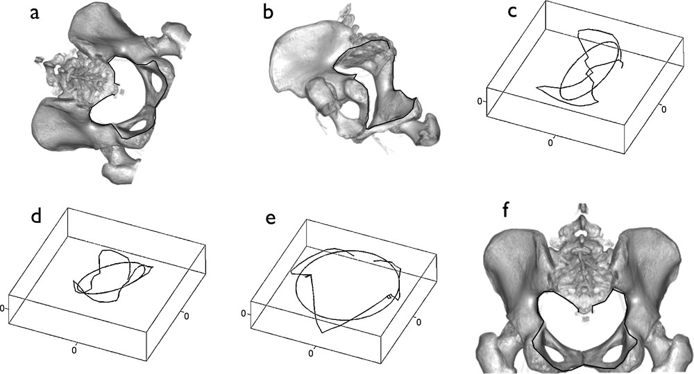
Overview of the algorithm. (a) and (b) show two CT scan bone volume rendering on which the pelvic outlet has been outlined (black line). (b) is a mathematically rotated and rescaled image of (a). Corresponding pelvic outlets alone and first elliptical Fourier descriptor are shown respectively in (c) and (d). Notice that orientation and area of these ellipses are different for the two images. The normalization-reorientation steps of the algorithm are then performed on the two contours, by making the first harmonic the reference plane of the contour and by normalizing the distances in order to set the area of the first harmonic equal to 1. The same contour, illustrated in (e), is obtained after the normalization-reorientation steps of the algorithm, whether starting from the (c) or (d) contours. Finally, the new pelvic outlet is represented in (f) superimposed to the initial bone structures.

4.2 Morphometrical analysis of the foramen magnum contour in a murine model of X-linked hypohidrotic ectodermal dysplasia

X-linked hypohidrotic ectodermal dysplasia (XLHED) is a genetic disorder due to a mutation of Eda gene [29]. The clinical phenotype of individuals affected by HED is complex and associates hypotrichosis, dental agenesis and morphological defects, onychodysplasia and eccrine glands aplasia or hypoplasia, being the main cardinal features [30]. Craniofacial and anthropometric changes are also described in XLHED and consist in reduced and retrognatic maxilla, frontal prominence, cranial base modifications, reduced facial convexity and facial height with deficiencies in skeletal sagittal and transversal growth [31–33]. Although the tooth abnormalities in Tabby mutant mice (the murine model of XLHED) have been extensively studied, the characterization of the craniofacial complex has received less attention. Therefore from 3D microCT reconstructions of the skull, the contour of the foramen magnum (a 3D line) was quantified using 3D Elliptical Fourier analysis, allowing quantitative comparisons between Tabby specimens and their wild type controls.

EdaTa mice were generated from the inbred Ta strain B6CBACa Aw-J/A-EdaTa/J-XO (Jackson Laboratory, USA). Mice phenotype was identified according to external morphological criteria: bald patches behind ears and deformities in the distal portion of the tail for hemizygous males (EdaTa/Y), striping of the coat for heterozygous females (EdaTa/ + ). WT mice were generated by inbreeding wild-type animals derived from the B6129PF2/J strain considered as control for strains designated by B6. WT mice and Tabby heterozygous females and homozygous males were genotyped according to previously published protocols [34] through PCR amplification using specific forward and reverse oligonucleotides (3F-7R, 6F-8R and 5F-6R), derived from −3 kb to +1.9 kb murine genomic sequence surrounding exon 1 of the WT Eda gene. The presence of a deletion in Eda gene exon 1 was observed in Ta specimens, as the 6F-8R primers allowed for amplification only in Ta heterozygous females and WT. The expected genotype of each Ta mice was confirmed by the absence of the 5F-6R primed fragments in Ta males. Mice population sample included 24 specimens, seven hemizygous males (EdaTa/Y), six heterozygous females (EdaTa/ + ), six control WT females and five control WT males. All the specimens studied were adults (3-month-old mice). Mice were killed by intraperitoneal lethal injection of pentobarbital. The experimental protocol was designed in compliance with recommendations of the EEC (86/609/CEE) for the care and use of laboratory animals. The animals were fixed in 1:10 37% formol, 3:4 100% ethanol, and 3:20 distilled water solution for 15 days. Imaging of full heads was performed using a microCT system (eXplore CT 120, GE Healthcare, Waukesha, WI, USA). The protocol used acquired 360 views on 360°, at 100 kV, 50.0 mA, with an exposure time of 20 ms. The duration of one acquisition was less than 4 min. A Feldkamp algorithm of backprojection led to the reconstruction of a volume made of cubic voxels of 50 μm × 50 μm × 50 μm. Steps of the image analysis procedure were performed using MicroWiew (GE Healthcare, Waukesha, WI, USA). A 3D virtual reconstruction of the skull was computed using the isosurface volume rendering module with a threshold value set at 600 HU (Fig. 3). Each foramen magnum outline was then manually recorded as a series of 20 sampling points represented by their 3D Cartesian coordinates (Fig. 3). The degree of distinction among mouse strains was then assessed and displayed graphically using discriminant analysis performed with Statistica 7.1 software package (Statsoft Inc., Tulsa, OK, USA). Correlations between 3D elliptical Fourier descriptors and discriminant axes were calculated. The unbiased Mahalanobis D2 distances, corrected for unequal sample sizes between the centroids of each group were also calculated to express inter-mouse strains variability. The discriminant analysis of the elliptical descriptors was limited to the first four harmonics because the multivariate analysis was no more significant after these harmonics (WilksLamda values p ≥ 0.05). The first two discriminant functions (DF1, DF2) described 86.3% of the total variance, the first accounting for 80.9% of the total variance, the second DF for the remaining 5.4%. Illustrated in Fig. 3, hemizygous Ta males and heterozygous Ta females clearly departed from the corresponding WT groups as shown by the significant distances separating the EdaTa/Y and EdaTa/+ specimens from the other mice groups (Table 1). The greatest difference occurred between WT males and females illustrating the sexual dysmorphism. The lower difference occured between Ta females and corresponding WT as demonstrated by the inter-group distances illustrated in Fig. 3 and Table 1.

Figure 3
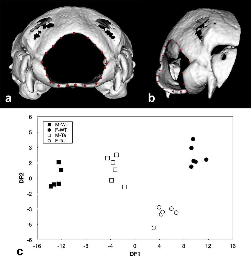
Isosurface 3D microCT reconstructions of wild type and Tabby mice skull. (a) posterior view and (b) postero-lateral view showing also the sampling points of the three-dimensional contour of the foramen magnum outlined in red. (c) discriminant analysis of the 4 first elliptical descriptors of the foramen magnum of the four mice groups (M-WT: wild type males, F-WT: wild type females, M-Ta: Tabby hemizygous males, F-Ta: Tabby heterozygous females).

	M-WT	F-WT	M-Ta	F-Ta
M-WT	0	518.3	114.3	326.1
F-WT	518.3	0	193.9	59.6
M-Ta	114.3	193.9	0	93.9
F-Ta	326.1	59.6	93.9	0

5 Discussion

The algorithm presented in this article makes use of the elliptical Fourier descriptors to reorient, rescale and compare three-dimensional curves. It makes use of the first harmonic to define an intrinsic Cartesian coordinate system in which Fourier descriptors, or alternatively coordinates, are computed. Potential applications of this algorithm are numerous but we focus the discussion to biological and medical examples. Our first application example demonstrates how the algorithm can be used to reorient and normalize 3D lines of the same pelvic bone anatomical structures after simulation of two different patient size and position from an X-ray CT exam. In biomedical imaging, comparison of sequential three-dimensional contours across time for the follow-up of a particular patient needs such steps of normalization and reorientation. In clinical practice, the algorithm can also be used to rescale, reorient, and compare two exams acquired in two different conditions, such as stress vs. rest in myocardial perfusion single photon emission computed tomography (compared to clinical existing nuclear medicine softwares where this step of reorientation is obtained manually). Alternatively, one may want to describe 3D anatomical lines to assess the feasibility of a certain procedure. For instance, in obstetrics, pelvimetry evaluates the size of pelvic inlet and outlet to know if a vaginal delivery is possible, or if a cesarean section is required. Once clinical, this assessment is now helped with CT-measurements but does not take into account the whole 3D contour information. It is well-known that these measurements have poor predictive value (see for example [35]). Extraction of the 3D line and its subsequent analysis with our algorighm may lead to precious information regarding the possiblity of vaginal delivery. More broadly, compared to manual anatomical landmarks and distances analysis, elliptical Fourier descriptors of bi-dimensional contours of anatomical structures (obtained for instance by X-ray planar projection) have demonstrated a great potential for shape comparison purposes [5–9]. However, elliptical Fourier descriptors of three-dimensional contours are more anatomically relevant, since most anatomical structures are three-dimensional. It can be used to sort animals for taxonomic purposes, or to study gene influence on phenotype as shown in our second example about cranial dysmorphoses in a murine model of XLHED. In this case, the 3D elliptical Fourier descriptors algorithm was applied to a particular 3D line of an open bone structure of the skull (the foramen magnum), allowing for a clear distinction between homozygous and heterozygous Ta mice and their WT controls. This particular example illustrates the interest of the proposed method for open anatomical structures like the foramen magnum whose three-dimensional morphology are generally difficult to analyze. Elliptical Fourier descriptors analysis applied to three-dimensional contours treats the shape as a single entity and allows retrieval of the entire anatomical profile. For better data reproducibility, automated three-dimensional contour detection from biomedical isotropic tomographic images should be preferred to manual extraction. Entire outlines of biological objects contours can be obtained from sets of non invasive digital isotropic tomographic images sources (CT or MRI images for instance). Based on differences in contrasts, many filtering and tresholding data processing softwares are able to trace automatically the 3D boundaries of particular anatomical structures. It avoids the difficulties of localizing specific landmarks, especially for open structures [36,37]. A whole automated and efficient shape analysis procedure could be then achieved starting with an extraction of 3D surface by volume rendering image processing software followed by a selection of singular aligned points on the surface as an input to the algorithm presented in this paper. This procedure could be of particular interest for automated screening in large scale mouse phenotyping programs. Finally, computational time is not a major concern given the speed of the algorithm.

6 Conclusion

The algorithm presented in this article computes, for the first time, the relations between the Fourier coefficients of a contour embedded in the three-dimensional space as a sum of ellipses and its corresponding geometric parameters. These relations are then used to create an algorithm for the rescaling and reorientation of 3D objects, and contour comparison. The usefulness of this algorithm is demonstrated for morphometrical comparison purposes using 3D anatomical profiles obtained from biomedical clinical and preclinical X-ray computed tomography.

Disclosure of interest

The authors declare that they have no conflicts of interest concerning this article.

Acknowledgments

The authors thank P. Choquet, M. Schmittbuhl and R. Godefroy for helpful discussions. A special thank to F. Hubele for his help throughout this work.

Bibliographie

[1] Cosgriff, R.L. Identification of shape. Ohio State Univ. Res. Foudation, (ASTIA AD 274 792), 1960.

[2] G.H. Granlund Fourier Preprocessing for Hand Print Character Recognition, IEEE Trans. Comput., Volume 21 (1972), pp. 195-201

[3] F.P. Kuhl; R.C. Giardina Elliptic Fourier features of a closed contour, Comput. Graph. Image Process., Volume 18 (1982) no. 3, pp. 236-258

[4] C.T. Zahn; R.Z. Roskies Fourier Descriptors for Plane Closed Curves, IEEE Trans. Comp., Volume 21 (1972), pp. 269-281

[5] P.E. Lestrel Fourier descriptors and their applications in biology, Cambridge University Press, New York, 1997

[6] S.E. Bailey; J.M. Lynch Diagnostic differences in mandibular P4 shape between Neandertals and anatomically modern humans, Am. J. Phys. Anthropol., Volume 126 (2005), pp. 268-277

[7] D.J. Daegling; W.L. Jungers Elliptical Fourier analysis of symphyseal shape in great ape mandibles, J. Hum. Evol., Volume 39 (2000) no. 1, pp. 107-122

[8] F. Guy; H.T. Mackaye; A. Likius; P. Vignaud; M. Schmittbuhl; M. Brunet Symphyseal shape variation in extant and fossil hominoids, and the symphysis of Australopithecus bahrelghazali, J. Hum. Evol., Volume 55 (2008) no. 1, pp. 37-47

[9] S. Chen; P. Lestrel; W. Kerr; J. McColl Describing shape changes in the human mandible using elliptical Fourier functions, Eur. J. Orthodontics, Volume 22 (2000) no. 3, pp. 205-216

[10] P.E. Lestrel; W.J.S. Kerr Quantification of function regulator therapy using elliptical Fourier functions, Eur. J. Orthodontics, Volume 15 (1993) no. 6, pp. 481-491

[11] R. Marquis; F. Taroni; S. Bozza; M. Schmittbuhl Quantitative characterization of morphological polymorphism of handwritten characters loops, Forens. Sci. Intern., Volume 164 (2006) no. 2–3, pp. 211-220

[12] R. Marquis; F. Taroni; S. Bozza; M. Schmittbuhl Size influence on shape of handwritten characters loops, Forens. Sci. Intern., Volume 172 (2007) no. 1, pp. 10-16

[13] T.P. Wallace; P.A. Wintz An efficient three-dimensional aircraft recognition algorithm using normalized fourier descriptors, Comput. Graph. Image Process., Volume 13 (1980) no. 2, pp. 99-126

[14] A. Cuyt; J. Sijbers; B. Verdonk; D. Van Dyck Region and Contour Identification of Physical Objects, Appl. Num. Anal. Comput. Math., Volume 1 (2004), pp. 343-352

[15] F. Dufrenois Segmentation and motion analysis of 2D anf 3D objects using a flexible Fourier model, Trait. Signal, Volume 17 (2000), pp. 153-178

[16] Li, J. Three-dimensional shape modeling: segmentation, reconstruction and registration. PhD thesis, University of Michigan, 2002.

[17] Vranic, D.V., Saupe, D. 3D Shape Descriptor Based on 3D Fourier Transform. Proceedings of the EURASIP Conference on Digital Signal Processing for Multimedia Communications and Services (ECMCS 2001), 2001.

[18] M.F. Wu; H.T. Sheu Representation of 3D Surfaces by Two-Variable Fourier Descriptors, IEEE Trans. Pattern Anal. Mach. Intell., Volume 20 (1998) no. 8, pp. 858-863

[19] M. Zribi Description of three-dimensional gray-level objects by the harmonic analysis approach, Pattern Recogn. Lett., Volume 23 (2002), pp. 235-243

[20] C.S. Lin; C. Jungthirapanich Invariants of three-dimensional contours, Pattern Recogn., Volume 23 (1990), pp. 833-842

[21] P. Bose. The encoding and Fourier descriptors of arbitrary curves in 3-dimensional space. M. Sc. Thesis, University of Florida, 2000.

[22] H.A. Kowalski. A normalized elliptic Fourier analysis method for spatial ECG rhythm classification. Folia Cardiol.:SC-P017, 2005.

[23] M. Friess; F.J. Rohlf; H. Hsiao Quantitative assessment of human body shape using Fourier analysis, Three-Dimensional Image Capture and Applications VI, Volume 5302 (2004) no. 1, pp. 117-124

[24] Y. Jeong; R.J. Radke Reslicing axially sampled 3D shapes using elliptic Fourier descriptors, Med. Image Anal., Volume 11 (2007) no. 2, pp. 197-206

[25] Monnet, C., Zollikofer, C., Bucher, H., Goudemand, N. Three-dimensional Morphometric Ontogeny of Mollusc Shells by Micro-Computed Tomography and Geometric Analysis. Palaeontol. Elec.:Article Number 12.3.12A, 2009.

[26] Toshihiro, O. A study of ventricular motion in cardiac MRI using deformable models. Undergraduate honor thesis project, Ohio State University, 2007.

[27] H.T. Sheu; M.F. Wu Fourier descriptor based technique for reconstructing 3D contours from stereo images, Vis. Image Signal Process. IEE Proc., Volume 142 (1995) no. 2, pp. 95-104

[28] K. Arbter; W.E. Snyder; H. Burkhardt; G. Hirzinger Application of Affine-Invariant Fourier Descriptors to Recognition of 3-D Objects, IEEE Trans. Pattern Anal. Mach. Intell., Volume 12 (1990), pp. 640-647

[29] M.C. Vincent; V. Biancalana; D. Ginisty; J.L. Mandel; P. Calvas Mutational spectrum of the ED1 gene in X-linked hypohidrotic ectodermal dysplasia, Eur. J. Hum. Genet., Volume 9 (2001) no. 5, pp. 355-363

[30] M. Pinheiro; N. Freire-Maia Ectodermal dysplasias: a clinical classification and a causal review, Am. J. Med. Genet., Volume 53 (1994) no. 2, pp. 153-162

[31] S. Arslan; J. Devecioglu Kama; T. Ozer; I. Yavuz Craniofacial and upper airway cephalometrics in hypohidrotic ectodermal dysplasia, Dentomaxillofac. Radiol., Volume 36 (2007) no. 8, pp. 478-483

[32] F. Clauss; M.C. Manière; F. Obry; E. Waltmann; S. Hadj-Rabia; C. Bodemer; Y. Alembik; H. Lesot; M. Schmittbuhl Dento-craniofacial phenotypes and underlying molecular mechanisms in hypohidrotic ectodermal dysplasia (HED): a review, J. Dent. Res., Volume 87 (2008) no. 12, pp. 1089-1099

[33] E.L. Johnson; M.W. Roberts; A.D. Guckes; L.J. Bailey; C.L. Phillips; J.T. Wright Analysis of craniofacial development in children with hypohidrotic ectodermal dysplasia, Am. J. Med. Genet., Volume 112 (2002) no. 4, pp. 327-334

[34] P. Bourgeois; A.L. Bolcato-Bellemin; J.M. Danse; A. Bloch-Zupan; K. Yoshiba; C. Stoetzel; F. Perrin-Schmitt The variable expressivity and incomplete penetrance of the twist-null heterozygous mouse phenotype resemble those of human Saethre-Chotzen syndrome, Hum. Mol. Genet., Volume 7 (1998) no. 6, pp. 945-957

[35] M.V. Zaretsky; J.M. Alexander; D.D. McIntire; M.R. Hatab; D.M. Twickler; K.J. Leveno Magnetic resonance imaging pelvimetry and the prediction of labor dystocia, Obstet. Gynecol., Volume 106 (2005), pp. 916-926

[36] Costa, L., Cesar, R. Shape analysis and classification: theory and practice. Boca Raton, CRC Press, 2001.

[37] S. Judex; Y. Luu; B. Ozcivici; S. Lublinski; C. Rubin Quantification of adiposity in small rodents using micro CT, Methods, Volume 50 (2010), pp. 1-14

Commentaires - Politique