

1 Introduction
The measurement of tree growth with the purpose of relating it to environmental and genetic factors has long been the subject of intensive research, from a variety of perspectives, including dendrochronology [1] and wood technology [2]. While photosynthesis and the companion recycling of atmospheric carbon dioxide occur at the level of the leaves in trees, annual increments of the stem circumference, which are reflected by annual rings in temperate and boreal climates, and troughs and peaks in the fluctuations of wood density, depending on whether the wood is produced earlier or later in a given year, are more easily traceable indicators of tree growth [3–6].
The characterization of wood properties inside a tree stem [7–11] has motivated the development and use of a plethora of measurement techniques. Many of these are based on the X-ray technology: computed tomography (CT) scanning [12–17]; microdensitometry [18]; and others [19,20]. Rarely, though, was a three-dimensional (3D) analysis of the data really performed; when this was the case, the focus was on the detection of branch knots, known as rameal traces [16,17] and compression wood [21] in the tree stem, rather than the measurement of tree growth via wood density variations within and among annual rings. In two dimensions, an automated but essentially graphical procedure involving multiple processing stages has been proposed to generate tree-ring profiles from the CT image showing the cross-section of a piece of wood [22]; in one dimension, one curve of raw CT numbers showing peaks corresponding to different years, from bark to bark, has been presented in [23], together with one 2D CT image of the stem of a Pinus nigra tree at breast height.
Hereafter, we explain how measurements are possible in 3D by CT scanning stem sections (Fig. 1d,e). In doing so, we shall explore the content and nature of tree stem sections (Fig. 1b,c) and identify growth layers and rings in a large number of directions in 3D. After integration along the vertical axis z (over successive CT images), the resulting maps of means (Fig. 1f) and corresponding standard deviations of wood density estimates will be presented, with the horizontal x–y plane (perpendicular to the stem) as support. A novelty of our approach is that it allows the extraction of “virtual cores” (Fig. 1g) from the wood CT scan dataset, which in turn provides the basis for:
- (i) plotting curves of wood density estimates in multiple directions;
- (ii) measuring the width of annual rings in each direction;
- (iii) assessing the variations in ring width as a function of year and direction.
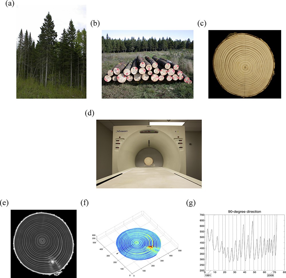
(Color online.) a: white spruce (Picea glauca (Moench) Voss) trees in a natural forest stand of Québec (Canada); b: logs of white spruce trees awaiting pick-up after harvesting; c: stem section of a white spruce tree, prepared for CT scanning (with a direction of reference indicated in pencil); d: same stem section as in (c), installed on the couch of the CT scanner (Toshiba XVision) prior to CT scanning; e: one of the 25 CT images constructed along the stem axis and used for further data analysis; f: map of means of wood densities estimated from the CT scan data (Fig. 2), for the stem section in (c) and (d); and g: curve of estimated wood densities for a “virtual core” with one-voxel diameter (Fig. 3).
For illustration, we use stem sections from two white spruce trees (see, e.g., Fig. 1a), with circular vs non-circular stem growth patterns. Then, we discuss the pros and cons of the approach and define the conditions of application for future studies. From the dendrochronological perspective, when the aim is back-forecasting the climate, we address the implications of measuring tree growth from radial wood cores instead of wood volumes (i.e. discs with a thickness) analyzed for their inner part rather than their surface [21], and make suggestions regarding possible field equipment for the on-site collection of CT scan data for the latter.
2 Materials and methods
The wood discs, for which results of graphical and quantitative analyses of CT scan data will be presented to illustrate the new approach proposed, are stem sections of two white spruces (Picea glauca (Moench) Voss), grown in natural forest stands of Québec (Canada) and harvested in October 2009 (Tree 1) and September 2009 (Tree 2). These two trees were chosen for their very different stem growth patterns (circular, Tree 1 vs non-circular, Tree 2), from a number of white spruces harvested the same year in a broader region (Tree 1: 45°26′11′′N, 70°54′45′′W; Tree 2: 46°45′25′′N, 79°04′41′′W). They grew in the same climatic zone (Nordic temperate) but a different vegetation area, composed of other white spruces and balsam firs (Abies balsamea (L.) Mill.) for Tree 1 vs trembling aspens (Populus tremuloides Michx.) and white birches (Betula papyrifera Marsh.) for Tree 2. They also differed in site topography, 14° slope exposure relative to magnetic north and at the bottom of a 5% slope (Tree 1) vs a 144° slope exposure and mid-way of an 8% slope (Tree 2).
The high-resolution X-ray CT scanner used in this study is the same as the one used in [24–26], where technological details about some of our previous plant science applications (i.e. canopies and wood sticks) can be found. In the CT scanning of Tree 1 and Tree 2 stem sections, the following parameter values were used: 50 mA (tube current), 120 kV (tube voltage), 1 mm (X-ray beam width), and 18 cm (field of view) for Tree 1 and 24 cm (field of view) for Tree 2; no zoom factor was applied. Using the Helical Scan option with a 0.3-mm thickness, CT images were first constructed every 0.3 mm in the tree stem direction (z-axis), each CT image (x–y plane) consisting of a 512 × 512 matrix of CT numbers. Then, CT numbers were converted to wood density estimates using the calibration equation, density = 0.993 × CT number + 1015, for not oven-dried wood in [12] (see also [26]); our wood samples were not oven-dried and the estimated 95% confidence interval for moisture content (4.6 ± 1.8%) included the lower bound of 6% in [12]. To capture the variability in 3D and represent it graphically, one map of means and one map of corresponding standard deviations (in the x–y plane) were computed from the wood density estimates obtained from 25 CT images (along the z-axis) for each of the two wood discs. The functions mean and std of the MATLAB programming language were used to compute 2D arrays of values of the two statistics, which were mapped with the function mesh (The MathWorks, Inc., Natick, MA, USA). The bark was excluded from the computations. For each wood disc, bark exclusion from map production was made by visual inspection of the 25 CT images, which were processed individually with the MATLAB function imtool. Specifically, since bark is much more dense than most of the interior part of the stem section with the exception of rameal traces, peripheral voxels appearing in white or very light grey in a CT image (see, e.g., Fig. 1e), thus, possessing very high CT numbers (i.e. high densities), were peeled out manually.
In order to compare directional variations, which involves quantitative analyses (see below), but also to demonstrate the multi-directionality, flexibility and fineness of the approach, eight “virtual cores” were extracted digitally from the 3D array of CT scan data collected for each wood disc; customized MATLAB programs were written for this. The extraction was performed horizontally (in the x–y plane) and included the x- and y-axes (both sides) as 4 of the 8 directions, plus the 4 diagonals, every 45° from an interior point used as centre for the stem at the height considered (see, e.g., the arrows in Fig. 2a,b); the definition of a location for the centre of the stem in a CT image was made graphically and numerically with a customized MATLAB graphical unit interface, by zooming in the central part of the raw CT image (see, e.g., Fig. 1e) and approximating it by a circle, the centre of this circle providing the centre of the stem to work with (see [22] for another procedure of pith detection, with multiple image processing steps). The extracted virtual cores can mimic cylinders with a given diameter; “mimic”, because of the discrete (by opposition to continuous) character of CT images, which are 512 × 512 matrices of CT numbers; it follows that these virtual cores are made of voxels (i.e. 3D extensions of pixels or parallelepiped rectangles). Mimicked cylinders could have a diameter of 5 mm or 12 mm (i.e. the diameter of “real cores” usually extracted on-site from the stem of standing trees in dendrochronological studies). Here, we chose to work with virtual cores with a one-voxel thickness (i.e. 0.3–0.35 mm for Tree 1, 0.3–0.47 mm for Tree 2), which facilitates the finding of limits for the annual growth rings in our work. Virtual cores of other sizes (i.e. ca. 5 mm and 12 mm in diameter) are considered in another study reported in a manuscript in preparation.
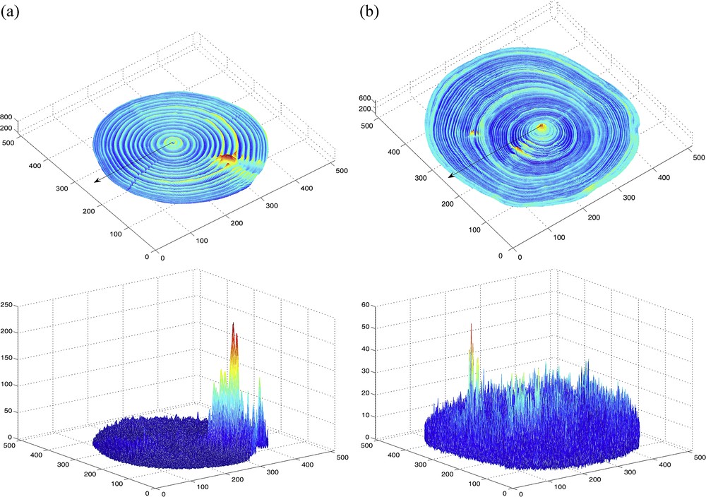
(Color online.) Maps of means (top) and corresponding standard deviations (bottom) in the x–y plane, computed from wood density estimates obtained from 25 CT images constructed along the z-axis, for a stem section of two white spruces (Picea glauca (Moench) Voss); the bark was digitally removed from the CT images and thus excluded from the computations; different colors are used in accordance to the values mapped, from lowest value (dark blue) to highest value (red) with light blue, green, yellow and orange in this order in-between, for intermediate values within the range of a given map (see values reported on the vertical axis). So-called (a) “Tree 1” and (b) “Tree 2” (see description in the text, Materials and methods section). In each of the two maps of means, the arrowed line indicates one of the eight directions in which the width of annual growth rings was measured (Fig. 3).
For each of the virtual cores extracted here, a curve made of wood density estimates was produced every 0.35 mm for Tree 1 (i.e. the field of view of 18 cm, divided by 512 ≈ 0.35 mm) and every 0.47 mm for Tree 2 (i.e. 24 cm divided by 512 ≈ 0.47 mm); a multiplicative factor, equal to square root of 2, applies for diagonal curves. Thus, 16 curves in total were produced, eight per wood disc all around the stem circumference. The beginning and end of annual growth rings for Tree 1 and Tree 2 were identified from the inter-peak distances in wood density estimates, following the calibration procedure of Manceur et al. [26; see Appendix] who also worked with white spruce stem samples, but sticks instead of discs. Curves were produced in order to cover the whole detectable period of growth on an annual basis for Tree 1, before its harvesting in 2009 (i.e. 18 years from 1991 to 2008, excluding the very first years of its lifetime); for Tree 2 (also harvested in 2009), the 15 years studied more closely, from 1950 to 1964, are those over which non-circularity in growth was the most apparent.
As for quantitative analyses, the coefficient of variation (CV), defined as the ratio of the sample standard deviation to the sample mean [27], was used as a unitless measure of dispersion (expressed as a percentage), to quantify the variation in annual growth ring with direction and assess the differences in that variation between Tree 1 and Tree 2. It was expected that under the non-circular stem growth scenario (Tree 2), CV values would be greater than under circularity (Tree 1).
3 Results
Important rules of interpretation must be given prior to starting to scrutinize the content of Fig. 2 (two maps of mean wood density estimates and two maps of standard deviations, one map of each type for Tree 1 and for Tree 2), in relation to the content of Fig. 3 (2 × 8 directional curves of wood density estimates for Trees 1 and 2). First of all, the colors (blue, green, yellow, orange, and red) and contrasts (dark/light) used in the maps of means and standard deviations are the default Jet options for the R2013a version of the MATLAB function mesh (The MathWorks, Inc., Natick, MA, USA). There is an increasing gradient in the mapped values with colors from blue to red, and contrasting colors (e.g., dark blue vs light blue) correspond to lower (dark color) and higher (light color) values, respectively. In a study like ours, very particular attention must be paid to the latter aspect, since it is well known [2] and this is clearly shown in the directional curves of Fig. 3: variation of wood density within annual growth rings is usually such that early wood has a lower density than late wood. As a result, early wood generally appears in dark blue in the top maps of Fig. 2 while late wood appears in light blue, green or yellow. On wood discs, however, the color of late wood is dark brown whereas early wood is light brown in temperate and boreal climates (see, e.g., Fig. 1c). If we had chosen to work with grey tones instead of colors, the same kind of care should have been taken because in classical CT image analysis, darker grey is conventionally used for lighter material (e.g., air is usually represented in black), and lighter grey, for denser material (e.g., white is used for rock or bone). We insist on these rules of interpretation because they are very important in wood CT scanning; this way, results will be correctly interpreted; and the explanations above were not given in [28], for example.
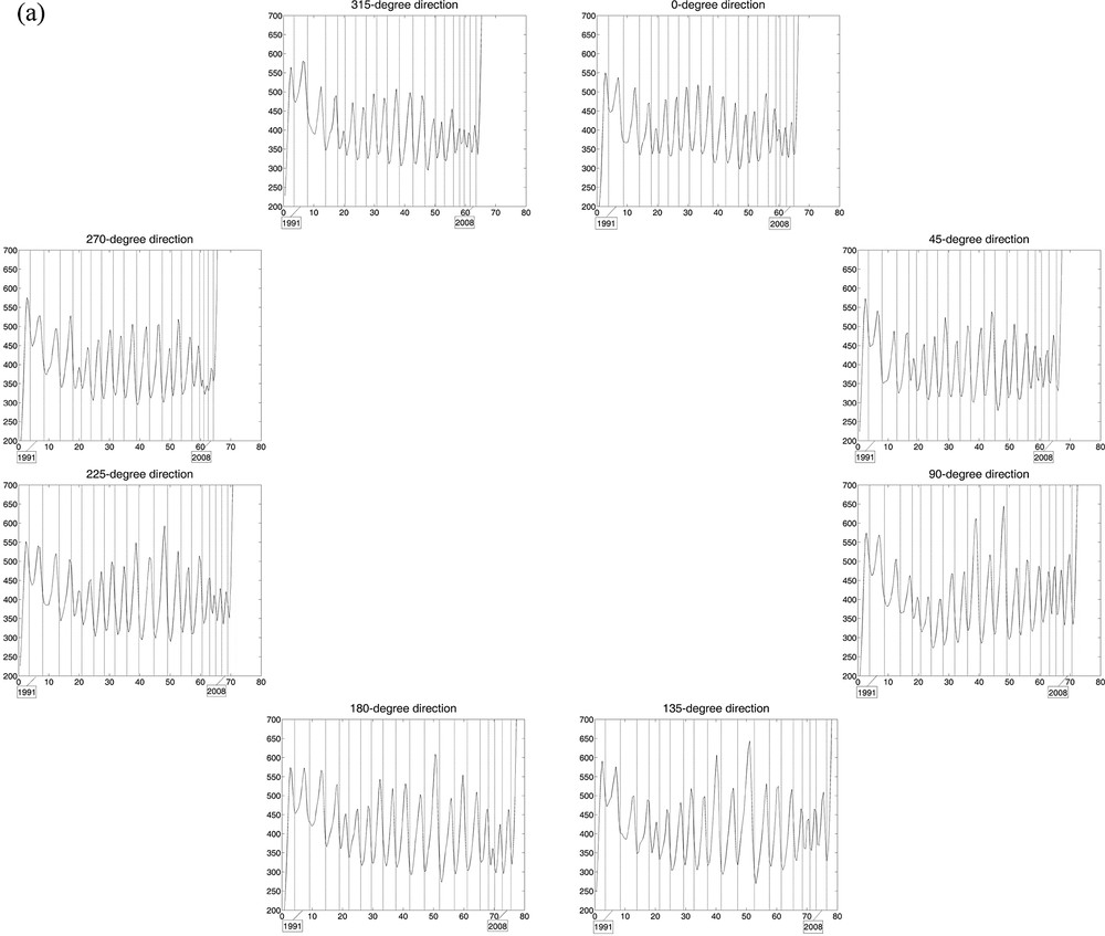
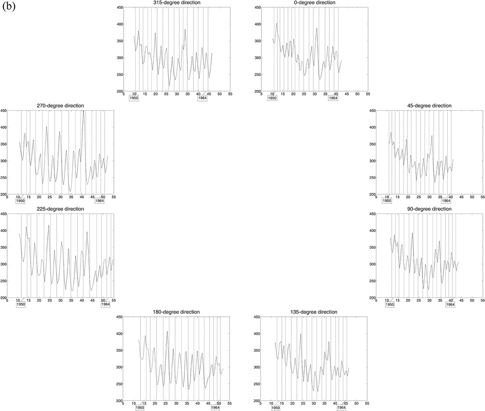
Curves of estimated wood densities for eight “virtual cores” with one-voxel diameter per stem section, with growth ring limits in filigree; the horizontal axis represents the distance (in mm) from an interior reference point. The cores were extracted digitally from the 3D array of collected CT scan data, every 45° including the x- and y-axes and the diagonals at the height considered. a: Tree 1, for which the limits of 18 central growth rings are represented in each of the eight directions; b: Tree 2, for which the limits of 15 central growth rings were drawn.
The map of means of estimated wood density for Tree 1 shows clear and consistent fluctuations within and among growth rings in all directions but a few (Fig. 2a, top panel), due to the presence of a portion of branch between two of the eight directions chosen to extract virtual cores and display curves in Fig. 3a; there is no such exception in the case of Tree 2 (Fig. 2b, top panel). The zone with highest wood density in the CT scanned stem section corresponds to a rameal trace for Tree 1 and the vicinity of the pith for Tree 2. The maps of standard deviations of estimated wood density (Fig. 2, bottom panels) provide a different type of multi-directional information, in terms of dispersion, about the growth of trees inside their stem. The zones of greater dispersion in wood density in the CT scanned stem section tend to correspond to the zones of higher mean wood density, especially for Tree 1 which is characterized by a wider range of wood density estimates (i.e. 200–800 against 200–600 for Tree 2); the greater dispersion of wood density near the knot in the case of Tree 1 is probably mostly due to the radial orientation of branches, which makes the CT number of a given voxel change from slice to slice.
In Fig. 3, the 2 × 8 curves of estimated wood densities, corresponding to the eight virtual cores extracted from the CT scan data collected for the two trees, reliably reproduce their growth pattern in the stem over time, circular for Tree 1 (over 18 years) vs non-circular for Tree 2 (over 15 years). The CVs calculated from the estimated ring widths per year among the 8 directions help quantify the differences in stem growth with direction between trees. For Tree 1, the mean CV value (± standard error) is 9.78% (± 0.98%), with minimum and maximum values of 4.96% and 18.02%, respectively; for Tree 2, the mean CV is 17.43% (± 1.18%), with minimum and maximum of 11.61% and 25.17%.
4 Discussion
Computed tomography (CT) scanning, as a technology based on matter density variations in a body or an object, is a very natural way to explore the interior of a tree stem because of the succession every year within a growth ring of early wood and late wood, characterized by tracheids with large size and lumen but thin walls and tracheids with small size and lumen but thick walls, respectively. As a result, early wood is less dense than late wood [2], and this appears clearly, already in raw CT images (see, e.g., [13], and Fig. 1e here). Further quantitative and statistical analyses of numerical wood CT scanning data (i.e. CT numbers) have been limited so far, except in [26] but this recent study, which also allowed some tree-ring profiling, was for bark-to-bark sticks instead of wood discs as stem sections.
Estimated wood density maps produced from CT scan data of stem sections (Fig. 2) depict tree growth in a unique and novel manner in all directions within a certain volume, while including a measure of vertical variability (along the stem). By comparison, the approach based on the analysis of wood cores, mimicked here with the extraction of virtual cores from the CT scan data, may provide an incorrect representation of tree growth when this is anisotropic (i.e. dependent on direction), whatever diameter is used for the cores (e.g., one-voxel here; 5 mm and 12 mm in Beaulieu et al., unpublished); such a situation corresponds to non-circular growth rings (e.g., Tree 2). Since this approach has been followed in dendroclimatology for decades [29] and although several trees per site and more than one tree-ring series per tree were generally used to construct site chronologies, it is natural to be intrigued and in view of our results (Fig. 3), to start thinking about the reliability or representativeness of some of the site chronologies that have been built in the past. Assuming Tree 2 was chosen to build a site chronology (despite the anisotropy of its growth inside the stem, likely due to non-climatic factors), the use of tree-ring series in the directions of 0, 45, 90, and 315° or of 0, 225, 270, and 315° from the direction of reference would give very different results (Fig. 3b); more specifically, differences could vary in sign and size, and be > 30% between ring widths of the same year.
For a given combination of electric and non-electric parameter values, such as tube current, tube voltage and beam width, the spatial resolution achieved with an X-ray technology is dependent on the volume analyzed with it in one exposure to X-rays; that volume is proportional to the field of view, which can be reduced by the use of a zoom factor. Techniques alternative to CT scanning can attain spatial resolutions as fine as a few tens of microns [18–20] or even the cell [30], but not in 3D or for complete wood discs as those of Tree 1 and Tree 2 CT scanned here; X-ray microtomography achieves very fine resolutions in 3D (scale of resolution: μm) but for very small samples (scale of observation: mm), and this technology falls under CT scanning [31]. With a CT scanner like ours (i.e. a Toshiba XVision), spatial resolution can be decreased to 50 μm by CT scanning the sample in several parts first and then merging the CT scan datasets; this has been done with wood sticks [26] and could be done with wood discs.
Moisture content, whether homogenously or heterogeneously distributed over the wood sample, has an effect on the outcome of its CT scanning. If heterogeneously distributed, a distinction must be made between sensible or meaningful differences in moisture content, such as in juvenile wood in first growth rings vs in mature wood in later growth rings in green wood [13], and artefact moisture content effects due to ill-controlled storage conditions or the presence of fungi in parts of the wood sample. In our study, the white spruce trees were harvested in the fall of 2009 and stem sections were stored and air-dried in a closed room until they were CT scanned in winter 2012. To obtain density estimates, the same calibration equation (see Materials and methods) holds for a broad range of wood moisture contents (6–117%). For wood samples that have been oven-dried, a slightly different calibration equation applies [12].
In closing, most of the CT scanners are not mobile, which obliges researchers to CT scan stem sections of harvested trees, as we did it. If there were more CT scanners of small size that could be moved and brought to a forest stand for being strapped on live trees [28], the procedures that we have presented for data analysis would apply, as one of the calibration equations in [12] holds for green wood. Of course, a well-defined protocol aimed at limiting variations in temperature and moisture content between sampling sites and times would be required for such “field wood CT scanning”, to provide sufficient accuracy of measurements and allow comparison between studies. This notwithstanding, we have provided evidence for a new approach to study tree growth rings and relate their width to climate with an appropriate resolution-to-size ratio.
Disclosure of interest
The authors declare that they have no conflicts of interest concerning this article.
Acknowledgements
The financial assistance of the Natural Sciences and Engineering Research Council of Canada through a Discovery Grant to PD under Grant No Nserc Rgpin 138514-10 and of the Canadian Wood Fibre Centre through research fund awarded to JB is gratefully acknowledged. The authors are grateful to Sébastien Clément, Patrick Laplante, Roger Gagné and Philippe Labrie (Canadian Forest Service) for tree documentation and to an anonymous reviewer for constructive comments on our original submission.
.