Formation of banded vegetation patterns resulted from interactions between sediment deposition and vegetation growth

Tousheng Huang; Huayong Zhang; Liming Dai; Xuebing Cong; Shengnan Ma

doi:10.1016/j.crvi.2018.01.008

Ecology/Écologie

Formation of banded vegetation patterns resulted from interactions between sediment deposition and vegetation growth

Tousheng Huang ^1,² ; Huayong Zhang ¹ ; Liming Dai ² ; Xuebing Cong ¹ ; Shengnan Ma ¹

¹ Research Center for Engineering Ecology and Nonlinear Science, North China Electric Power University, Beijing 102206, PR China
² Industrial Systems Engineering, University of Regina, Regina, SK S4S 0A2, Canada

Comptes Rendus. Biologies, Volume 341 (2018) no. 3, pp. 167-181.

Résumé

This research investigates the formation of banded vegetation patterns on hillslopes affected by interactions between sediment deposition and vegetation growth. The following two perspectives in the formation of these patterns are taken into consideration: (a) increased sediment deposition from plant interception, and (b) reduced plant biomass caused by sediment accumulation. A spatial model is proposed to describe how the interactions between sediment deposition and vegetation growth promote self-organization of banded vegetation patterns. Based on theoretical and numerical analyses of the proposed spatial model, vegetation bands can result from a Turing instability mechanism. The banded vegetation patterns obtained in this research resemble patterns reported in the literature. Moreover, measured by sediment dynamics, the variation of hillslope landform can be described. The model predicts how treads on hillslopes evolve with the banded patterns. Thus, we provide a quantitative interpretation for coevolution of vegetation patterns and landforms under effects of sediment redistribution.

Métadonnées

Reçu le : 2017-09-29
Accepté le : 2018-01-25
Publié le : 2018-03-01

PMID

DOI : 10.1016/j.crvi.2018.01.008

Mots clés : Hillslope landform, Vegetation pattern formation, Banded patterns, Turing instability, Geomorphic processes

Affiliations des auteurs :

Tousheng Huang ^{1, 2} ; Huayong Zhang ¹ ; Liming Dai ² ; Xuebing Cong ¹ ; Shengnan Ma ¹

@article{CRBIOL_2018__341_3_167_0,
     author = {Tousheng Huang and Huayong Zhang and Liming Dai and Xuebing Cong and Shengnan Ma},
     title = {Formation of banded vegetation patterns resulted from interactions between sediment deposition and vegetation growth},
     journal = {Comptes Rendus. Biologies},
     pages = {167--181},
     publisher = {Elsevier},
     volume = {341},
     number = {3},
     year = {2018},
     doi = {10.1016/j.crvi.2018.01.008},
     language = {en},
}

TY  - JOUR
AU  - Tousheng Huang
AU  - Huayong Zhang
AU  - Liming Dai
AU  - Xuebing Cong
AU  - Shengnan Ma
TI  - Formation of banded vegetation patterns resulted from interactions between sediment deposition and vegetation growth
JO  - Comptes Rendus. Biologies
PY  - 2018
SP  - 167
EP  - 181
VL  - 341
IS  - 3
PB  - Elsevier
DO  - 10.1016/j.crvi.2018.01.008
LA  - en
ID  - CRBIOL_2018__341_3_167_0
ER  -

%0 Journal Article
%A Tousheng Huang
%A Huayong Zhang
%A Liming Dai
%A Xuebing Cong
%A Shengnan Ma
%T Formation of banded vegetation patterns resulted from interactions between sediment deposition and vegetation growth
%J Comptes Rendus. Biologies
%D 2018
%P 167-181
%V 341
%N 3
%I Elsevier
%R 10.1016/j.crvi.2018.01.008
%G en
%F CRBIOL_2018__341_3_167_0

Tousheng Huang; Huayong Zhang; Liming Dai; Xuebing Cong; Shengnan Ma. Formation of banded vegetation patterns resulted from interactions between sediment deposition and vegetation growth. Comptes Rendus. Biologies, Volume 341 (2018) no. 3, pp. 167-181. doi : 10.1016/j.crvi.2018.01.008. https://comptes-rendus.academie-sciences.fr/biologies/articles/10.1016/j.crvi.2018.01.008/

Version originale du texte intégral

1 Introduction

Banded vegetation patterns exist widely in the world's ecosystems [1–6]. Such patterns comprise alternating bands of vegetation and bare ground, and are a characteristic feature of landscapes in many arid and semiarid areas [7–9]. These patterns have been widely studied through field investigations and theoretical analysis due to their widespread occurrence and special features [10].

A large number of hypotheses aim to comprehend the self-organization of these patterns [8,10–14]. One important hypothesis addresses the nonlinear feedback between plant biomass and water resources of runoff–runon systems [15,16]. Rainfall on bare soil bands barely infiltrates, but runs downhill into vegetated bands and accumulates. Plant biomass can be greatly magnified in vegetated areas due to uptake of soil water by plant roots.

Many dynamic models based on feedback mechanisms of plant biomass and water resources have been established [8,10,11,15–20]. Two are regarded as core spatial vegetation-water models. The Klausmeier model addresses the formation of banded vegetation patterns in semiarid regions driven by feedback between biomass and water infiltration [8]. The second, proposed by HilleRisLambers et al. [15] and Rietkerk et al. [11], describes the water budget in detail as both soil and surface water. This model produces vegetation patterns of spots, labyrinths, gaps, and regular bands, dependent on rainfall and slope gradient [11]. The two models and their modified versions provide significant understanding of core mechanistic processes of vegetation pattern formation [21].

In the published literature on banded vegetation patterns, only a few researchers have considered the importance of micro-geomorphic processes [22–27]. Processes of soil erosion, sediment transport, and sediment deposition exert great influence on vegetation growth. A substantial amount of sediment is intercepted, trapped, and accumulated at vegetation patches [28,29]. Because the topsoil layer varies with soil erosion and sediment deposition, vegetation growth is greatly affected. Field observations and laboratory experiments show that soil erosion and/or sediment deposition may promote the development of banded vegetation patterns on hillslopes [1,28,30–35].

Considering the influences of soil variation aids understanding of the formation of banded vegetation patterns. For vegetation growth on hillslopes, soil factors dominate the water resource. First, mineral nutrition and water resources necessary for vegetation growth are stored in the soil layer. Second, soil provides a stable environment for vegetation growth. Disturbance of the soil by geomorphic processes leads to variations of water resources and nutrients for plants, affecting vegetation growth [36]. Thornes [37] and Zhang [38] proposed theoretical frameworks regarding the ecology of erosion and eroded ecosystems. From this perspective, focusing on influences of soil variation is more important than considering water resource effects on banded vegetation patterns. Moreover, soil thickness can be directly measured, reflecting variations of microtopography in banded patterns.

The natural world indeed offers examples of the formation of vegetation patterns resulting from soil variation. As observed by Gallart et al. [32], “grassed stairs” and terracette patterns are common features in the central Pyrenees. Generally, the terracettes are restricted to an altitudinal range between 1700 and 2700 m. The total plant cover of the terracette surfaces is often between 30 and 35%, and the main building species are bunchgrasses such as Festuca eskia, Festuca gautieri, Sesleria cerulea, etc. The growth habit of bunchgrasses results in a slow radial growth rate of the clump, and therefore the bunch reaches a high plant density in the clumps, while leaving areas of bare soil among them. On flat or gentle slopes, the bunch growth habit produces a mosaic of more or less circular random phases. As the gradient becomes steeper, bunches become roughly semicircular and tend to connect together, giving a pattern of continuous treads and risers following topographic contours.

Based on the ecological observations of Gallart et al. [32], substantial sediments are transported by overland flow and settle in vegetated areas intercepted by vegetation. Under negative influences of the accumulated sediments, small-scale vegetation bands appear on hillslopes. Thus, the interactions between sediment deposition and vegetation growth promote self-organization of banded vegetation patterns on hillslopes. However, little literature exists on this topic. A dynamic model of sediment deposition and vegetation growth on hillslopes is still needed for quantitative analysis of patterns that result from such interactions.

In this study, a spatial dynamic model is established, describing dynamics of sediment deposition and vegetation growth, based on the field observations of Gallart et al. [32]. The model aims to theoretically investigate the mechanism for the spontaneous emergence of banded patterns and stepped topography in the above case of the central Pyrenees as well as other cases with similar interactions and environmental conditions. Considering the characteristics of vegetation growth and sediment deposition in the above case, the spatial model is parameterized and utilized to simulate and analyze the formation process of banded vegetation patterns. However, it should be noted that the Pyrenees sites studied here are characterized by more humid climatic conditions than the arid and semiarid regions studied in much of the literature. Therefore, the model developed here is site-specific in that the feedbacks between sediment deposition and vegetation growth are likely more important than those between water redistribution and vegetation growth in the emergence of banded vegetation.

In developing the dynamic model of sediment deposition and vegetation growth, Thornes’ thought, which directly integrates geomorphic and ecological processes [37,39–41], is accepted. Via Turing analysis and numerical simulations on the model, the process and mechanism of formation of banded vegetation patterns are addressed. In this research, banded vegetation patterns describe a stable state of spatially heterogeneous vegetation, which shifts under influences exerted by sediment accumulation on vegetation growth.

2 Development of the model for formation of banded vegetation patterns

The dynamic model describes the formation of banded vegetation patterns on hillslopes, which is mainly influenced by the interactions between sediment deposition and vegetation growth.

2.1 Interactions between sediment deposition and vegetation growth

Although many studies use the feedback mechanisms between water and biomass to interpret vegetation pattern formation, vegetation pattern formation can result from the interactions between geomorphic processes and vegetation growth [23,27,37,40,42–44]. Hoffman et al. [45] concluded that the “current mathematical models of pattern formation in drylands typically consider only an infiltration-vegetation feedback and root augmentation growth as driving mechanisms, yet patterns of sedimentation and erosion on the soil surface have a strong effect on hydrological processes, stressing the need to introduce a soil-vegetation and an annual-shrub feedback.”

Gallart et al. [32] observed that banded vegetation patterns in high-mountain terracettes were common features on steep slopes between 1700 and 2700 asl in the central Pyrenees. As described by Gallart et al. [32], terracettes “show a convex downslope riser of bunchgrasses retaining a tread of almost bare soil upslope.” The authors understood the formation of such patterns as the result of the interactions between bunchgrass growth and geomorphic processes. Following the approach of Gallart et al. [32], the present study focuses on the mechanism of interactions between sediment deposition and vegetation growth and its effects on the formation of banded vegetation patterns in ecosystems.

As described in Gallart et al. [32], “most terracettes show coarse deposits which cannot be transported by runoff.” In this situation, two aspects are suggested: on the one hand, sediment deposition takes place along with other sediment processes including soil erosion and sediment transfer; on the other hand, sediment deposition prevails over other sediment processes in the formation of banded vegetation patterns. To quantitatively describe the effects of such sediment movement on formation of banded patterns; in this study, we consider a net sediment deposition, which is the result of sediment deposition subtracting the effects of soil erosion and sediment transfer. In the following, “sediment deposition” as used in this paper always means “net sediment deposition”. Net sediment deposition in nature is manifested by actual thickness of the sediment layer.

As a natural micro-geomorphic process, sediment deposition on hillslopes is promoted by vegetation cover [46,47], agreeing with tread retention in the terracettes of Pyrenees [32]. Persistent accumulation of sediments can negatively influence vegetation growth. Gallart et al. [32] showed that sediment deposition restricted vegetation growth and led to pronounced mortality and lower seedling establishment. The negative influence of sediment deposition is reflected in two aspects. First, sediment deposition affects the properties and structure of soil, leading to deterioration of the environment in which vegetation grows [48]. Second, the sediment layer formed by deposition of sand or even coarser sediments hardly retains water, which infiltrates quickly and runs away as subsurface flow [32]. Lack of water resource in the sediment/soil layer results in slow growth or mortality of vegetation.

In this study, the sediment deposition process is considered as the main dynamic process that promotes formation of banded patterns. The feasibility of this proposition is addressed:

• As shown by Gallart, infiltration rates on the deposited area are as high as 700 mm/h, and water quickly exfiltrates at the feet of vegetated bands. Water redistribution is therefore determined by the property of sediments;
• As the sediment deposits increase, the surface where plants establish rises. Since the water runs as subsurface flow, the root systems of plants need to change to reach the water. The sediment deposition thus influences vegetation establishment and how vegetation absorbs the water resource.

More importantly, sediment deposition changes the runoff–runon mechanism [25]. Deposit of coarse sediments causes a small difference in infiltration rate between bare and vegetated areas. Sediment deposition is more informative than water redistribution in describing the pattern formation.

Sediment deposits act as substitutes of the soil layer for vegetation establishment. The contents of mineral materials and organic matter vary between sediment deposits. Since sediment deposition results in a change in nutrient distribution, sediment deposition is considered as a more comprehensive index than water resources.

Sediment deposition, instead of water redistribution, is thus considered as the main dynamic process. Sediment redistribution is dynamic, affects vegetation growth, and promotes the formation of banded patterns. In describing the formation of banded patterns, Gallart et al. [32] did not even consider water redistribution. Thornes [37] and Burg et al. [41] also emphasized effects of sediment movement on vegetation growth, without considering water redistribution.

The relationship between vegetation biomass and deposited sediment is interactive. Two assumptions of the dynamic model are proposed:

• Sediment deposition is the main dynamic process that affects vegetation pattern formation. The influence of water resource is considered as a subfactor included in the sediment deposition;
• Sediments are transported by un-concentrated runoff. Banded vegetation cannot appear in landscapes with incised rills and gullies, where flow concentration precludes generation of sheet flow [26].

Interactions between sediment deposition and vegetation growth are briefly emphasized:

• Vegetation promotes sediment deposition. Higher plant biomass brings more sediment deposits;
• Accumulated sediment harms vegetation growth in that it deters its development into a homogeneous cover.

Therefore, a dynamic model that integrates vegetation growth and sediment deposition is established to study the self-organization of the banded vegetation patterns. In fact, direct integration of ecological and geomorphic processes is supported in Thornes’ work, which provides a framework for the ecology of erosion from a holistic perspective [37,40]. This model is applied to theoretically explain the self-organization of banded patterns and stepped topography in the case of the central Pyrenees as well as other cases with similar interactions and environmental conditions.

2.2 Model establishment

The dynamic model has two state variables for vegetation growth and sediment deposition. Thickness of the deposited sediment layer, S, is used for net sediment deposition, and ground plant biomass, V, is used for vegetation growth. The change of S is related to natural deposition and promotion of deposition by plant biomass. The change in V is determined by the intrinsic growth of vegetation and negative effect of accumulated sediments on vegetation.

The spatial distribution of S and V on planar hillslopes is considered. With the introduction of spatial terms, the model describes rates of change of S and V in both space and time. The dynamics of the two state variables are expressed in the following equations, after which a detailed interpretation of the equations is provided.

\frac{\partial S (x, y, t)}{\partial t} = A_{0} (1 - \frac{S (x, y, t)}{S_{m}}) + b V (x, y, t) + u \frac{\partial S (x, y, t)}{\partial x},

(1a)

\frac{\partial V (x, y, t)}{\partial t} = h V (x, y, t) (1 - \frac{V (x, y, t)}{V_{m}}) - p S (x, y, t) + d (\frac{\partial^{2}}{\partial x^{2}} + \frac{\partial^{2}}{\partial y^{2}}) V (x, y, t) .

(1b)

In Eq. (1a), A₀(1–S/S_m) describes the net sediment deposition process. A sediment resource term A₀ represents the rate of net sediment deposition per unit of time. The parameter S_m is the maximal thickness of the sediment layer on bare ground. Since the rise of the sediment layer changes the routing of runoff and reduces the rate of sediment deposition, A₀S/S_m encompasses the self-damping of the sediment deposition process. Based on the assumption that the increase in sediment deposition caused by vegetation is simply proportional to plant biomass, bV is proposed. The parameter b is dependent on how plants retard the flow and trap sediments [29]. Sediment movement is kept with the flow and can be modeled by the convection term u∂S/∂x, where u is determined by the slope gradient. This convection term describes the deposited sediment flux along the downslope direction.

In Eq. (1b), a classic logistic growth term hV (1 − V/V_m) is used to describe plant biomass growth. h is the intrinsic vegetation growth rate and V_m is the maximum ground plant biomass given the ratio of actual to potential evapotranspiration [37]. The negative effect of deposited sediments on vegetation is modeled by a simple linear term pS. The lateral growth of vegetation is modeled by a diffusion term $d (\partial^{2} V / \partial x^{2} + \partial^{2} V / \partial y^{2})$ , where d is a diffusion coefficient for plant biomass [8,11,15]. Table 1 provides interpretations and units of all the variables and parameters shown in Eq. (1).

Table 1

Symbol	Interpretation	Units	Reference value	Source
S	Thickness of deposited sediment layer	cm	–	–
V	Ground plant biomass	kg·m⁻²	–	–
t	Time	Day	–	–
x, y	Space	dm	–	–
A ₀	Maximal rate of sediment deposition at S = 0	cm·day⁻¹	0.01	Descheemaeker et al. [60], Mabit et al. [61]
S _m	Maximal thickness of deposited sediment layer on bare ground	cm	20	Descheemaeker et al. [60], Mabit et al. [61]
b	Increased thickness of sediment layer per unit biomass	m²·cm·kg⁻¹·day⁻¹	0.005∼0.11	–
h	Maximal vegetation growth rate at V = 0	day⁻¹	0.005	Klausmeier [8], Gilad et al. [16]
V _m	Maximal ground plant biomass	kg·m⁻²	2	Thornes [39]
p	Decreased plant biomass per unit deposited sediments	kg·m⁻²·cm⁻¹·day⁻¹	0.00005	–
u	Speed of deposited sediment flux along the downslope	dm·day⁻¹	0.01	–
d	Plant dispersal rate	dm²·day⁻¹	0.01	Gilad et al. [16]

In Eq. (1), we apply simple linear terms bV and pS as specific functions to describe the interactions between vegetation and sediment deposition. It should be noted that many other functional forms satisfying the above assumptions can be used to describe the interactions and the results are not sensitive to the exact functional forms. With the employment of the model described by eq. (1), we now can investigate the formation of banded vegetation patterns generated on hillslopes from interactions between sediment deposition and vegetation growth. Theoretical analysis proves that this model can generate heterogeneous vegetation patterns and determine conditions for pattern formation. Numerical simulations are performed to form banded vegetation patterns.

3 Conditions for Turing bifurcation and banded pattern formation

For ecological significance, dynamics of the two state variables, S and V, should be restricted in the region S ≥ 0, V ≥ 0. Also, all the parameters in the model such as A₀, S_m, b, u, h, V_m, p, d, should be positive.

The first step in analyzing how the model generates banded vegetation patterns is to determine stationary states of the non-spatial system in which the space derivatives of eq. (1) are set to zero. By solving the equations of the two nullclines, ∂S/∂t = 0, ∂V/∂t = 0, i.e.

A_{0} (1 - \frac{S}{S_{m}}) + b V = 0,

(2a)

h V (1 - \frac{V}{V_{m}}) - p S = 0 .

(2b)

Three cases of stationary states corresponding to different parameter conditions can be described as follows:

• when Δ < 0, no stationary state exists for vegetation and deposition;
• when Δ = 0 and hA₀/pbS_m > 1, there exists a unique positive stationary state denoted by E_c (S_c, V_c), where S_c = S_m(1 + bV_c/A₀) and V_c = V_m(1–pbS_m/hA₀)/2;
• when Δ > 0 and hA₀/pbS_m > 1, two positive stationary states exist, denoted by E₁(S₁,V₁) and E₂(S₂,V₂), where S_1,2 = S_m(1 + bV_1,2/A₀) and $V_{1,2} = V_{m} (1 - p b S_{m} / h A_{0} \pm \sqrt{Δ / h^{2}}) / 2$ (here set V₁ > V₂).

In these three cases, the expression of Δ is described by

Δ = {(\frac{p b S_{m}}{A_{}} - h)}^{2} - \frac{4 h p S_{m}}{V_{m}} .

(3)

By the method of the Jacobian matrix, the local stability of stationary states in different cases is analyzed. The Jacobian matrix associated with the non-spatial system can be expressed by

J (S, V) = [\begin{array}{c} - \frac{A_{0}}{S_{m}} & b \\ - p & h (1 - \frac{2 V}{V_{m}}) \end{array}] .

(4)

The expressions of the stationary states are substituted into Eq. (4) and the two eigenvalues of the Jacobian matrix are calculated. The signs of the two eigenvalues λ₁ and λ₂ determine local stability of corresponding stationary states. Through these steps, the local stability of various stationary states is determined:

• The two eigenvalues of E_c satisfy λ₁λ₂ = 0. At this stationary state, the dimension of the non-spatial system can be reduced to one. In this case, E_c is a saddle-node point;
• For stationary state E₂, the two eigenvalues satisfy λ₁λ₂ < 0. The positive and negative eigenvalues reveal that E₂ is a saddle point;
• For stationary state E₁, the two eigenvalues satisfy λ₁λ₂ > 0. There are three cases for the local stability of E₁. Since $λ_{1} + λ_{2} = p b S_{m} / A_{0} - A_{0} / S_{m} - \sqrt{Δ}$ , when $p b S_{m} / A_{0} > A_{0} / S_{m} + \sqrt{Δ}$ , E₁ is an unstable node or unstable focus. When $p b S_{m} / A_{0} < A_{0} / S_{m} + \sqrt{Δ}$ , E₁ is a stable node or stable focus. When $p b S_{m} / A_{0} = A_{0} / S_{m} + \sqrt{Δ}$ , the situation is complicated because the non-spatial system may go through a Hopf bifurcation. Therefore, the local stability of E₁ cannot be determined without given specific values of the parameters.

Analyzing spatial system (1) can occur after obtaining the stable stationary state, which demonstrates that the vegetation can survive in the environments of deposited sediments. Moreover, the stable stationary state E₁ implies that system (1) is also stable under spatially homogeneous perturbations. However, when spatially heterogeneous perturbations at this stationary state exist, the homogeneous stationary state may be unstable. Such a property determines the occurrence of Turing's instability and the formation of banded patterns of system (1).

Starting from the spatially stable homogeneous stationary state, a small but spatially heterogeneous amount of plants and sediment is added or removed. If these perturbations diverge with time, the system (1) will enter a new spatial state, implying Turing instability [15]. The perturbation equations at a spatially homogeneous stable stationary state E₁ are expressed as:

S (x, y, t) = S_{1} + s (x, y, t),

(5a)

V (x, y, t) = V_{1} + v (x, y, t) .

(5b)

Substituting the perturbed equations into the system (1) gives

\frac{\partial s (x, y, t)}{\partial t} = - \frac{A_{0}}{S_{m}} s (x, y, t) + b v (x, y, t) + u \frac{\partial s (x, y, t)}{\partial x},

(6a)

\frac{\partial v (x, y, t)}{\partial t} = - p s (x, y, t) + h (1 - \frac{2 V_{1}}{V_{m}}) v (x, y, t) + d (\frac{\partial^{2} v (x, y, t)}{\partial x^{2}} + \frac{\partial^{2} v (x, y, t)}{\partial y^{2}}) .

(6b)

Expanding the small space-time heterogeneous perturbation in Eqs. (5) around the stable stationary state in Fourier space gives the following form of the perturbations:

s (x, y, t) = \bar{s} (t) e^{i (l_{1} x + l_{2} y)},

(7a)

v (x, y, t) = \bar{v} (t) e^{i (l_{1} x + l_{2} x)},

(7b)

where l₁ and l₂ are wavenumbers, and

i = \sqrt{- 1}

. Substituting (7) into (6) gives

\frac{d \bar{s} (t)}{d t} = (- \frac{A_{0}}{S_{m}} + i u l_{1}) \bar{s} (t) + b \bar{v} (t),

(8a)

\frac{d \bar{v} (t)}{d t} = - p \bar{s} (t) + (h (1 - \frac{2 V_{1}}{V_{m}}) - d (l_{1}^{2} + l_{2}^{2})) \bar{v} (t) .

(8b)

The Jacobian matrix of the ordinary differential eq. (8) is

J_{2} = [\begin{array}{c} - \frac{A_{0}}{S_{m}} + i u l_{1} & b \\ - p & h (1 - \frac{2 V_{1}}{V_{m}}) - d (l_{1}^{2} + l_{2}^{2}) \end{array}] .

(9)

Since the eigenvalues of matrix (9) determines the occurrence of Turing instability [15], the following characteristic equation can be calculated:

{(λ (l_{1}, l_{2}))}^{2} - (γ + n) λ (l_{1}, l_{2}) + γ η + b p = 0,

(10)

where

γ = - \frac{A_{0}}{S_{m}} + i u l_{1},

η = h (1 - \frac{2 V_{1}}{V_{m}}) - d (l_{1}^{2} + l_{2}^{2}) .

The dispersion relation is obtained:

λ (l_{1}, l_{2}) = \frac{1}{2} (γ + η \pm \sqrt{ε + i θ}),

(11)

where

ε = {(- \frac{A_{0}}{S_{m}} - η)}^{2} - u^{2} l_{1}^{2} - 4 b p,

θ = 2 u l_{1} (- \frac{A_{0}}{S_{m}} - η) .

Straightforward manipulation yields:

Re (λ (l_{1}, l_{2})) = \frac{1}{2} (- \frac{A_{0}}{S_{m}} + η + \frac{j}{\sqrt{2}} \sqrt{\sqrt{ε^{2} + θ^{2} + ε}}),

(12)

and

Im (λ (l_{1}, l_{2})) = \frac{1}{2} (u l_{1} + \frac{j}{\sqrt{2}} sign (θ) \sqrt{\sqrt{ε^{2} + θ^{2}} - ε}),

(13)

where j = ±1.

As described above, Turing's instability and patterned vegetation need two conditions to be satisfied. First, system (1) is stable to spatially homogeneous perturbations, i.e. the non-spatial system has a locally stable stationary state. E₁ satisfies this condition when $p n S_{m} / A_{0} < A_{0} / S_{m} + \sqrt{Δ}$ . Second, system (1) is unstable to spatially heterogeneous perturbations, i.e. the perturbed system (6) (or (8)) is unstable. At least one Re (λ(l₁, l₂)) must be larger than zero, i.e.

- \frac{A_{0}}{S_{m}} + η + \frac{1}{\sqrt{2}} \sqrt{\sqrt{ε^{2} + θ^{2}} + ε > 0} .

(14)

By direct calculation, this condition for the occurrence of Turing's instability and banded patterns is:

u > \frac{A_{0} - S_{m} η}{S_{m} l_{1}} \sqrt{- \frac{b p S_{m}}{A_{0 η}}} - 1 .

(15)

4 Numerical analyses

The results provided in Section 3 reveal that the spatial model of vegetation growth and sediment deposition yields banded vegetation patterns with proper parameters. However, the dynamical behaviors of the spatial model are difficult to obtain theoretically. It is thus necessary to perform numerical analyses, the most reliable approach with satisfactory accuracy and efficiency in comprehensively investigating characteristics of the model with feasible parameters.

Numerical analyses mainly focus on the stable stationary state and banded vegetation patterns. Three aspects of numerical simulations are performed:

• cases of stationary states in the phase space and possible bifurcations of the stationary states for different parameters;
• extensive simulations on parameter conditions of emerging banded vegetation patterns based on theoretical analysis;
• display of banded patterns with given parameters and their possible analysis.

Table 1 provides parameter reference values for numerical simulations. For various situations in numerical simulations, the parameter values may be changed around these reference values. The reference values of some parameters (A₀, S_m, h, V_m, d) are literature-based, while values of other parameters (b, p, h) are mathematically determined according to the conditions for the occurrence of Turing patterns. Using these values, numerical simulations are performed analogously to real cases.

Stability analysis on the non-spatial model proves the existence of stationary states. These states imply stable or unstable establishment of vegetation covers in depositional areas. Moreover, the stability of stationary states varies with parameter changes. Fig. 1 shows six possible cases of stationary states with different groups of parameters in phase diagrams. The stationary state E₁ can either be attracting (the stable node in Fig. 1a and the stable focus in Fig. 1b) or repelling (weakly repelling equilibrium in Fig. 1c, unstable focus in Fig. 1d, and the unstable node in Fig. 1e). Simultaneously, stationary state E₂ is always a saddle in the five cases represented by Fig. 1a–e. For Fig. 1f, E₁ and E₂ merge together into the saddle-node E_c.

Fig. 1
Various cases of stationary states in the S–V space. E₁ is a (a) stable node, (b) stable focus, (c) weakly repelling equilibrium, (d) unstable focus, and (e) unstable node, whereas E₂ is always a saddle in these five graphs. In (f), the two stationary states merge into a saddle-node E_c. a: b = 0.005; b: b = 0.0157; c: b = 0.0571, h = 0.013; d: b = 0.0165; e: b = 0.0182; f: b = 0.018377. Other parameter values are listed in Table 1.

The dynamic behavior of stationary state E₁ presents gradual changes among the six cases, as the value of any one parameter continuously varies. Changes suggest two types of bifurcations that appear in the interactions between sediment deposition and vegetation growth described in Eq. (1). The saddle-node bifurcation occurs at the transformation between E_c and E_1,2. When the stationary state E₁ transforms from stable focus into unstable focus, the Hopf bifurcation generates a weakly repelling equilibrium. The Hopf bifurcation indicates a sudden shift between two different dynamic outcomes, namely, that vegetation will either stably exist or die in depositional environments.

The bifurcation diagrams for parameters A₀, b, h, and p are plotted to better comprehend them. As shown in each graph of Fig. 2, two branches of the stationary states, E₁ and E₂, are present. Due to the Hopf bifurcation, E₁ transforms between stable states and unstable states. Meanwhile, as a result of saddle-node bifurcation, saddle-branch E₂ is always at an unstable state.

Fig. 2
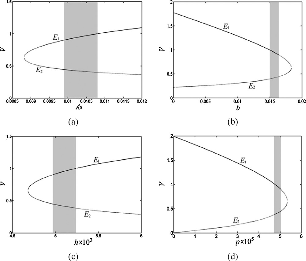
Bifurcation diagrams of the non-spatial model for (a) A₀, (b) b, (c) h, and (d) p. The solid lines describe stable states and the dashed lines describe unstable states. The shaded areas show the parameter range necessary for Turing instability occurrence and pattern formation. Parameter values are given in Table 1, b = 0.0162.

The saddle-node bifurcation provides parameter values for the appearance of coexisting stationary states between vegetation and deposited sediments. In Fig. 2, the parameter values at which saddle-node bifurcation occurs are A_0s = 8.82×10⁻³, b_s = 1.84×10⁻², h_s = 4.68×10⁻³, and p_s = 5.34×10⁻⁵. More importantly, the Hopf bifurcation determines critical values at which a sudden shift occurs between the vegetated and bare ground states. The critical values are A_0H = 9.90×10⁻³, b_H = 1.64×10⁻², h_H = 4.96×10⁻³, and p_H = 5.04×10⁻⁵. Only when A₀ > A_0H, b < b_H, h > h_H or p < p_H, can a stable vegetation cover exist and banded patterns be observed.

Emergence of banded vegetation patterns requires Turing instability. According to the analysis provided in Section 3, the parameters must satisfy $Re (λ (0,0)) < 0$ and $Re (λ (l_{1}, l_{2})) > 0$ when l₁ and/or l₂ are not equal to zero. From eq. (12), satisfying the latter condition requires 2 V₁ < V_m. Therefore, as shown in Fig. 2, a value range for each parameter is simulated. The shaded area in each graph represents this value range, describing a necessary combination of A₀, b, h, p, S_m and V_m for Turing's instability. The parameter ranges described in Fig. 2 are A_0H < A₀ < 1.08×10⁻², 1.50×10⁻² < b < b_H, h_H < h < 5.24×10⁻³, and 4.72×10⁻⁵ < p < p_H.

Considering the necessary conditions for Turing's pattern (i.e. Δ > 0, $h (1 - 2 V_{1} / V_{m}) - A_{0} / S_{m} < 0$ , and 2 V₁ < V_m), two cases of region diagrams are plotted for possible vegetation patterns for the non-spatial system (Fig. 3). In each region diagram, three parameter areas, homogeneous vegetation, no vegetation, and banded vegetation, are separated. Homogeneous vegetation implies that the S–V system exhibits a state of uniform vegetation biomass density. No vegetation is defined by the absence of a stationary state or an unstable one. Turing instability and banded vegetation occur in the parameter area enclosed by C1 and C2 or C3 and C2. From combination of α, β and δ, the value range of any needed parameter(s) for vegetation pattern formation can be easily calculated.

Fig. 3
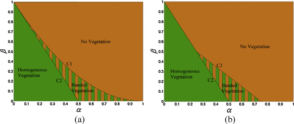
Regions diagrams for the non-spatial system. In each graph, three parameter areas, homogeneous vegetation, no vegetation, and banded vegetation, are separated. α = pbS_m/hA₀, β = 4pS_m/hV_m, δ = A₀/hS_m, C1 is β = (α−1)², C2 is β = −2α + 1, and C3 is β = 2(δ − 1) α + (1 − δ²). (a) δ ≥ 1, (b) δ < 1.

The ranges of parameters u and d for emerging banded vegetation patterns demand simulation of the dispersion relation. As shown in Fig. 4, Re (λ(l₁, l₂)) first increases and then drops as wavenumber l₁ increases. When the vertex point of the curve Re (λ(l₁, l₂)) is above zero, i.e. u > u_c or d < d_c, the spatial model generates banded vegetation patterns. The threshold values u_c and d_c imply that the slope gradient and the plant dispersal rate determine pattern formation.

Fig. 4
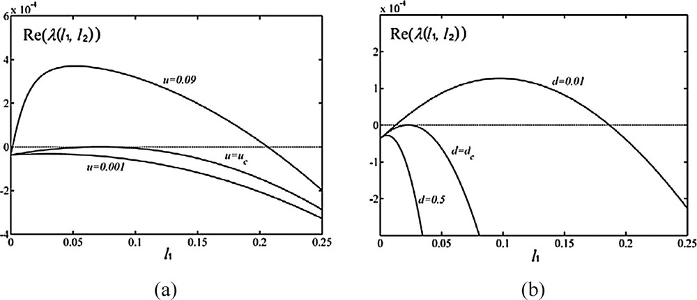
Changing Re (λ(l₁, l₂)) with variation parameters u and d. When Re (λ(l₁, l₂)) is larger than zero, banded vegetation patterns emerge. b = 0.0162, l₂ ₌ 0, and other parameter values are listed in Table 1, u_c = 0.0032 and d_c = 0.099.

With the parameters selected, numerical simulations are provided through discretizing partial differential equations of system (1) in two-dimensional space. The first-order upwinding finite difference scheme is applied to discretize the convection term and finite difference approximation to the diffusion term. An explicit Euler method is applied for the time integration with a time step size Δt = 0.05[day] and space step size Δh = 2[dm] [49]. The space and time scale is averaged for the Euler method. Spatial vegetation patterns are shown in a rectangular domain including 100 × 100 grid elements, representing 20 [m] × 20 [m]. Periodic boundary conditions are employed in the pattern simulations [8]. Initial conditions are given as perturbing 9% of the grid elements in stable homogeneous vegetation and letting biomass in these grid elements equal zero.

Fig. 5 shows the evolution of the banded vegetation pattern at 6, 55, 165, and 494 years, with given parameters. In Fig. 5a, b, and c, the vegetated patches grow laterally to gradually generate parallel vegetation bands. These vegetation bands are perpendicular to the flow direction. Fig. 5d shows a completely developed banded vegetation pattern. Moreover, this banded pattern oscillates in time and migrates in the upslope direction.

Fig. 5
Self-organization of regular banded vegetation pattern on planar slopes. b = 0.0162 and other parameter values are given in Table 1. a: t = 2000; b: t = 20,000; c: t = 60,000; d: t = 180,000. The downslope direction is from left to right in each graph and in the pattern graphs below.

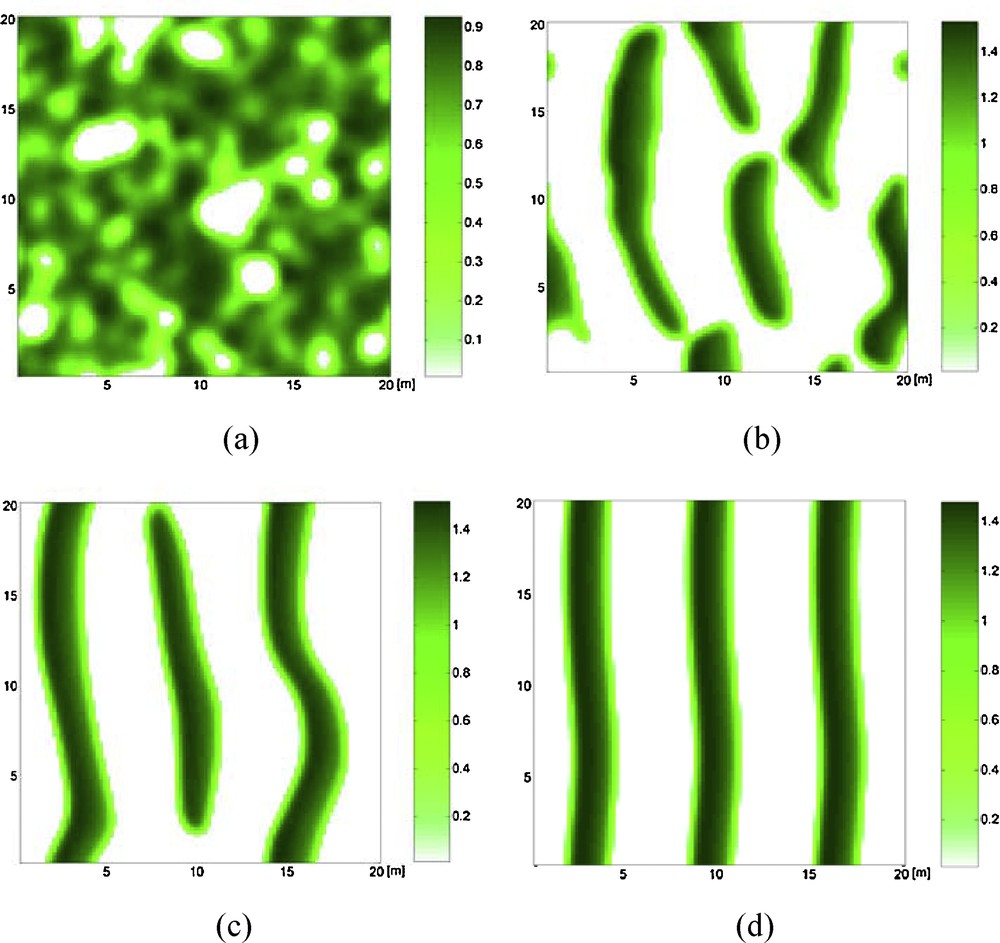
Fig. 6 shows how the change of sediment deposition process influences vegetation pattern features. As shown in Fig. 6a–b, the rate of sediment deposition doubles. Accordingly, the wavelength of the banded pattern decreases, but the number of vegetation bands increases. Fig. 6c–d show that decreasing S_m leads to a similar consequence. Results in Fig. 6 reveal that sediment deposition acceleration results in decreasing wavelength in banded vegetation patterns. Moreover, there is a time lag before the stable pattern is reached.

Fig. 6
Variation of vegetation patterns as the sediment deposition process changes. A₀ = 0.02, b = 0.034, a: t = 20,000; b: t = 180000, and A₀ = 0.02, b = 0.105, S_m = 10; c: t = 20,000; d: t = 360,000, and other parameter values are listed in Table 1.

A phenomenon of the banded pattern formation is shown in Fig. 7. The parameters presented in this case imply that the stationary state E₁ is unstable (see Fig. 1d) and that the Turing instability cannot appear. However, the banded vegetation pattern emerges from the dynamic influences of system (1) on the boundary S = 0 and V = 0. Since S and V must be positive for practical ecological sense, S or V is set to zero when each value becomes negative in the simulations. This results in self-organization of a banded vegetation pattern on the slopes. Moreover, the formation of banded patterns is accelerated, with the lag time in their formation reduced to about 439 years.

Fig. 7
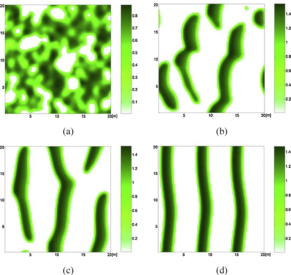
Self-organization of banded vegetation pattern when Turing instability does not occur. b = 0.0165 and other parameter values are given in Table 1. a: t = 2000; b: t = 20,000; c: t = 60,000; d: t = 160,000.

When the patterns of S and V are observed along the downslope direction, waves of plant biomass and sediment layer are found. Fig. 8a shows the alternating bands of vegetation and bare ground along the downslope direction. The horizontal line represents the plant biomass at the stable stationary state. Plant biomass at vegetation bands is much higher than at the stable stationary state. Asynchronism between the peak of vegetation bands and the bottom of sediment bands reveals the lag in the effect of interactions between sediment deposition and vegetation growth.

Fig. 8
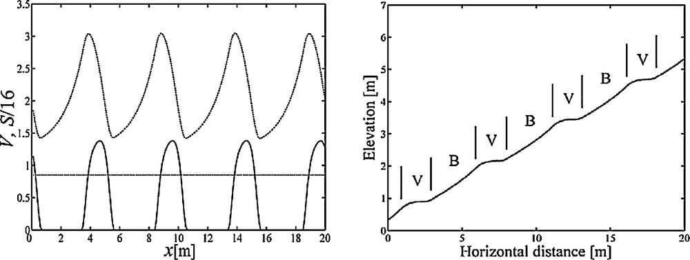
a: the regular patterns of S and V along the downslope direction. The lower wave represents plant biomass and the other wave is the sediment layer. The horizontal line represents plant biomass at E₁; b: longitudinal profile of a banded vegetation pattern and hillslope landform. The gradient of the hillslope is given as 25%. V: vegetated area; B: bare area. Parameter values are the same as in Fig. 6a–b.

To show the banded vegetation pattern on hillslopes, Fig. 8b is plotted. For analogy to the real pattern in the central Pyrenees, we chose a particular hillslope gradient (25%), as recorded in Gallart et al. [32] to plot Fig. 8b. Fig. 8b shows similar characteristics with the vegetation patterns described in literature. First, alternation of vegetated areas and bare areas is demonstrated. Second, the deposited sediments trapped in vegetated areas lead to the formation of treads on hillslopes. With the demonstration in Fig. 8b, the coevolution of vegetation patterns and landforms is quantitatively described in this study.

5 Discussion

Vegetation pattern formation on hillslopes mainly results from the balance of positive and negative feedback between resources for plants and plant biomass [10,11,16,50,51]. Since erosion and sediment deposition disturb the soil layer, affecting resources stored for plants, the spatial distribution of plant biomass is greatly influenced. This also leads to the formation of banded vegetation patterns [28,32,52].

Field investigations show that natural formation of banded vegetation patterns in the central Pyrenees is related to sedimentation on hillslopes and interactions between deposition and vegetation growth [32]. We determined that banded vegetation patterns self-organize when model parameters assume proper values (see the conditions for pattern formation described in Section 3). Using feasible parameter values provided in the literature (see Table 1), numerical simulations are performed analogously to real cases, and the main characteristics of banded pattern formation are quantitatively described.

Banded vegetation patterns were also discovered on semi-natural and abandoned land in the upper Guadalentín basin in southeastern Spain [34]. Cammeraat and Imeson found a strong interrelationship between plant development, sediment deposition, and soil surface crusting, leading to the development of fine-scale banded vegetation structures in degraded lands, dominated by Plantago albicans. At much lower slope positions, sediment deposition clearly becomes more and more important, and blankets of silt-sized material are deposited there. A thick silty crust is present, and the land shows bare and strongly crusted soils alternating with bands of P. albicans, developed in a direction parallel to the contours, at a more or less regular interval. The small bands of plants act as a sediment trap during the rare periods of overland flow, when silty sediments are transported downslope. Due to the accumulation of mainly fine-soil material and some organic debris, micro-topographical steps are also developed, coinciding with the bands of P. albicans. Directly under the small steps, erosion takes place during overland flow, creating small steep cuts in the surface with a height of about 2 cm, exposing coherent layered silts. Cammeraat and Imeson [34] suggested that the vegetation banding and resultant stepped topography were closely related to dynamics of sediment deposition. However, patterns described by Gallart et al. [32] and Cammeraat and Imeson [34] resulted from sediment deposits of different properties.

The field survey cases as described in Gallart et al. [32] and Cammeraat and Imeson [34] provide evidence of banded vegetation patterns that we can model. As can be seen from Figures 5 through 7, banded patterns of vegetation are completely developed under the conditions considered. Development of vegetation bands can be quantitatively described with this model. Employing the model, we found the following ecologically significant results:

• Decrease/increase of the sediment layer leads to increase/reduction of biomass in vegetation bands. Peaks of vegetation bands correspond to the thinnest parts of sediment layer. However, the lagging effect results in asynchronism between vegetation and sediment bands;
• Plants at boundaries of upslope vegetation bands suffer from negative effects of deposited sediments. This ultimately restricts the lateral growth of vegetation patches, and restriction results in the formation of parallel vegetation bands.

Considering ecosystem features, the simulated wavelengths and the real patterns are compared. Wavelengths of vegetation bands in simulated banded vegetation patterns range from 1.6 m to 2.5 m. The range observed by Gallart et al. [32] was from 0.2 m to 5 m, while Cammeraat and Imeson [34] reported wavelengths of 1.2 m in average. Thus, our simulated results are comparable.

Emergence and migration of vegetation bands require unidirectional runoff flow and sloped terrains [8,9,11,13,53]. Vegetation band formation is not directly dependent on slope gradient. Since sediment deposition is the main dynamic process in pattern formation, blocking of runoff flow and interception of sediments are important factors.

Field investigators have reported sediment deposition as being important for vegetation pattern formation [34,52,54,55]. These patterns also are formed by different mechanisms [7,56,57]. Bryan and Oostwoud Wijdenes [31], and Bryan and Brun [33] postulated that these bands result from positive effects of accumulated sediments in depositional zones. Interference factors such as overgrazing and fire lead to fragmentation of vegetation bands in nature.

The spatial vegetation-sediment model considers the effectiveness of sediment fluxes in the formation of banded vegetation. In contrast, the Klausmeier model considers the striped vegetation patterns to be generated merely by interactions between vegetation growth and water resources [8]. Sediment fluxes are more effective in forming banded patterns than water fluxes because water must be restored in soil before absorption. Redistribution of water in forming banded vegetation patterns is regarded as a consequence of disturbing soil layers by sediment deposition.

The important role of sediment fluxes in determining vegetation pattern formation is widely recognized, and many studies have contributed to the literature on this topic [25,28,45,52,58]. However, still few models are documented in the literature for predicting the coevolution of vegetation patterns and hillslope landforms [26,32,45,59]. Based on previous studies, the research reported here makes improvements. Directly integrating sediment flux and vegetation growth in a dynamic model allows the coevolution of vegetation patterns and hillslope landforms be calculated explicitly [32,37,41]. By comparing our work with that of Gallart et al., the effects of parameter variations on the coevolution and the characteristics of vegetation patterns and landforms can be quantitatively determined.

6 Conclusion

Formation of banded vegetation patterns on hillslopes, as an effect of sediment deposition, is investigated theoretically and numerically. With the consideration of the interactions between sediment deposition and vegetation growth, a relevant and novel spatially dynamic model is thus developed. To the best of our knowledge, such a model describing banded pattern formation on hillslopes due to sediment deposition has not yet appeared in the literature.

In this study, the analysis of Turing mechanisms has led to determination of the parameter conditions for the occurrence of banded vegetation patterns. Numerical simulations based on the model established simulate the self-organization process of the patterns under different conditions. Vegetation bands are found perpendicular to the direction of sediment flux. Also, with the model established, it is evident that treads on hillslopes emerge with the evolution of vegetation bands. The coevolution of banded vegetation patterns and landforms due to the interactions between sediment deposition and vegetation growth, as described quantitatively with the model, agrees with the field observations reported in the literature.

Disclosure of interest

The authors declare that they have no competing interest.

Acknowledgments

The authors would like to acknowledge with great gratitude the support of National Major Science and Technology Program for Water Pollution Control and Treatment (No. 2017ZX07101-002), the Fundamental Research Funds for the Central Universities (No. JB2017069), the China Scholarship Council (No. 201206730024), and the Chinese Natural Science Foundation (Project 39560023 to H.Z.). The authors also would like to thank the anonymous referees for their carefulness, helpful comments and suggestions, which greatly improved this paper.

Bibliographie

[1] G.E. Wickens; F.W. Collier Some vegetation patterns in the Republic of the Sudan, Geoderma, Volume 6 (1971), pp. 43-59 | DOI

[2] F. van der Meulen; J.W. Morris Striped vegetation patterns in a Transvaal savanna, Geo-Eco-Trop, Volume 3 (1979), pp. 253-266

[3] J.A. Mabbut; P.C. Fanning Vegetation banding in arid Western Australia, J. Arid Environ., Volume 12 (1987), pp. 41-59

[4] A. Mauchamp; S. Rambal; J. Lepart Simulating the dynamics of a vegetation mosaic: a spatialized functional model, Ecol. Model., Volume 71 (1994), pp. 107-130 | DOI

[5] J. Thiéry; J.-M. d’Herbès; C. Valentin A model for simulating the genesis of banded patterns in Niger, J. Ecol., Volume 83 (1995), pp. 497-507 | DOI

[6] M.F. Bekker; G.P. Malanson Linear forest patterns in subalpine environments, Prog. Phys. Geogr., Volume 32 (2008), pp. 635-653 | DOI

[7] L.P. White Vegetation stripes on sheet wash surfaces, J. Ecol., Volume 59 (1971), pp. 615-622 | DOI

[8] C.A. Klausmeier Regular and irregular patterns in semiarid vegetation, Science, Volume 284 (1999), pp. 1826-1828 | DOI

[9] J.A. Sherratt An analysis of vegetation stripe formation in semi-arid landscapes, J. Math. Biol., Volume 51 (2005), pp. 183-197 | DOI

[10] A.I. Borthagaray; M.A. Fuentes; P.A. Marquet Vegetation pattern formation in a fog-dependent ecosystem, J. Theor. Biol., Volume 265 (2010), pp. 18-26 | DOI

[11] M. Rietkerk; M.C. Boerlijst; F. van Langevelde; R. HilleRisLambers; J. van de Koppel; L. Kumar; H.H.T. Prins; A.M. de Roos Self-organization of vegetation in arid ecosystems, Am. Nat., Volume 160 (2002), pp. 524-530 | DOI

[12] N. Barbier; P. Couteron; R. Lefever; V. Deblauwe; O. Lejeune Spatial decoupling of facilitation of facilitation and competition at the origin of gapped vegetation patterns, Ecology, Volume 89 (2008), pp. 1521-1531 | DOI

[13] M. Rietkerk; J. van de Koppel Regular pattern formation in real ecosystems, Trends Ecol. Evol., Volume 23 (2008), pp. 169-175 | DOI

[14] N. Ursino Above and below ground biomass patterns in arid lands, Ecol. Model., Volume 220 (2009), pp. 1411-1418 | DOI

[15] R. HilleRisLambers; M. Rietkerk; F. van den Bosch; H. Prins; H. de Kroon Vegetation pattern formation in semi-arid grazing systems, Ecology, Volume 82 (2001), pp. 50-61 (10.1890/0012-9658(2001)082[0050:VPFISA]2.0.CO;2)

[16] E. Gilad; J. von Hardenberg; A. Provenzale; M. Shachak; E. Meron Ecosystem engineers: from pattern formation to habitat creation, Phys. Rev. Lett., Volume 93 (2004), p. 098105 | DOI

[17] J. Esteban; V. Fairén Self-organized formation of banded vegetation patterns in semi-arid regions: a model, Ecol. Complexity, Volume 3 (2006), pp. 109-118 | DOI

[18] S. Thompson; G. Katul; S.M. McMahon Role of biomass spread in vegetation pattern formation within arid ecosystems, Water Resour. Res., Volume 44 (2008), p. W10421 | DOI

[19] S. Kéfi; M.B. Eppinga; P.C. de Ruiter; M. Rietkerk Bistability and regular spatial patterns in arid ecosystems, Theor. Ecol., Volume 3 (2010), pp. 257-269 | DOI

[20] M. Baudena; M. Rietkerk Complexity and coexistence in a simple spatial model for arid savanna ecosystems, Theor. Ecol., Volume 6 (2013), pp. 131-141 | DOI

[21] F. Borgogno; P. D’Odorico; F. Laio; L. Ridolfi Mathematical models of vegetation pattern formation in ecohydrology, Rev. Geophys., Volume 47 (2009), p. RG1005 | DOI

[22] J.A. Ludwig; D.J. Tongway Spatial organisation of landscapes and its function in semi-arid woodlands, Australia, Landscape Ecol., Volume 1 (1995), pp. 209-215 | DOI

[23] D.R. Butler; G.P. Malanson; M.F. Bekker; L.M. Resler Lithologic, structural, and geomorphic controls on ribbon forest patterns in a glaciated mountain environment, Geomorphology, Volume 55 (2003), pp. 203-217 | DOI

[24] J.A. Ludwig; D.J. Tongway; S.G. Mardsen Stripes, strands or stipples: modelling the influence of three landscape banding patterns on resource capture and productivity in semi-arid woodlands, Australia, Catena, Volume 37 (1999), pp. 257-273 | DOI

[25] J.A. Ludwig; B.P. Wilcox; D.D. Breshears; D.J. Tongway; A.C. Imeson Vegetation patches and runoff-erosion as interacting ecohydrological processes in semiarid landscapes, Ecology, Volume 86 (2005), pp. 288-297 | DOI

[26] P.M. Saco; G.R. Willgoose; G.R. Hancock Eco-geomorphology of banded vegetation patterns in arid and semi-arid regions, Hydrol. Earth Syst. Sci., Volume 11 (2007), pp. 1717-1730 | DOI

[27] R.A. Marston Geomorphology and vegetation on hillslopes: interactions, dependencies, and feedback loops, Geomorphology, Volume 116 (2010), pp. 206-217 | DOI

[28] C. Valentin; J.M. d’Herbès; J. Poesen Soil and water components of banded vegetation patterns, Catena, Volume 37 (1999), pp. 1-24 | DOI

[29] R.P.C. Morgan Vegetative-based technologies for erosion control (Stokes; al. et, eds.), Eco- and Bio-Engineering: the Use of Vegetation to Improve Slope Stability, Springer, Netherlands, 2007, pp. 265-272

[30] G.A. Worral The Butana grass patterns, J. Soil Sci., Volume 10 (1959), pp. 36-53 | DOI

[31] R.B. Bryan; D. Oostwoud Wijdenes Field and laboratory experiments on the evolution of microsteps and scour channels on low-angle slopes, in: K.H. Schmidt, J. De Ploey (Eds.), Functional geomorphology: landform analysis models, Catena Supplement, Volume 23 (1992), pp. 133-161

[32] F. Gallart; J. Puigdefábregas; G. del Barrio Computer simulation of high mountain terracettes as interaction between vegetation growth and sediment movement, Catena, Volume 20 (1993), pp. 529-542 | DOI

[33] R.B. Bryan; S.E. Brun Laboratory experiments on sequential scour/deposition and their application to the development of banded vegetation, Catena, Volume 37 (1999), pp. 147-163 | DOI

[34] L.H. Cammeraat; A.C. Imeson The evolution and significance of soil-vegetation patterns following land abandonment and fire in Spain, Catena, Volume 37 (1999), pp. 107-124 | DOI

[35] D.R. Butler; G.P. Malanson; L.M. Resler Turf-banked terrace treads and risers, turf exfoliation, and possible relationships with advancing treeline, Catena, Volume 58 (2004), pp. 259-274 | DOI

[36] E.N. Mueller; J. Wainwright; A.J. Parsons Spatial variability of soil and nutrient characteristics of semi-arid grasslands and shrublands, Jornada Basin, New Mexico, Ecohydrology, Volume 1 (2008), pp. 3-12 | DOI

[37] J.B. Thornes The ecology of erosion, Geography, Volume 70 (1985) no. 3, pp. 222-236

[38] H. Zhang, Chinese Science and Technology Press, Beijing (1993), pp. 229-233

[39] J.B. Thornes, John Wiley and Sons Ltd, New York (1990), pp. 41-53

[40] J. Wainwright; A.J. Parsons The ecology of erosion (reprinted from Geography vol. 70, p. 222–35, 1985), Prog. Phys. Geogr., Volume 34 (2010) no. 3, pp. 399-408 | DOI

[41] D. Burg; D. Malkinson; G. Katriel; L. Wittenberg Modeling the dynamics of soil erosion and vegetative control—catastrophe and hysteresis, Theor. Ecol., Volume 8 (2015), pp. 67-79 | DOI

[42] G. Sanchez; J. Puigdefabregas Interactions of plant growth and sediment movement on slopes in a semi-arid environment, Geomorphology, Volume 9 (1994), pp. 243-260 | DOI

[43] L. Reinhardt; D. Jerolmack; B.J. Cardinale; V. Vanacker; J. Wright Dynamic interactions of life and its landscape: feedbacks at the interface of geomorphology and ecology, Earth Surf. Proc. Landforms, Volume 35 (2010), pp. 78-101 | DOI

[44] J.A. Dickie; A.J. Parsons Eco-geomorphological processes within grasslands, shrublands and badlands in the semi-arid Karoo, South Africa, Land Degrad. Dev., Volume 23 (2012), pp. 534-547 | DOI

[45] O. Hoffman; H. Yizhaq; B.R. Boeken Small-scale effects of annual and woody vegetation on sediment displacement under field conditions, Catena, Volume 109 (2013), pp. 157-163 | DOI

[46] L. Beuselinck; A. Steegen; G. Govers; J. Nachtergaele; I. Takken; J. Poesen Characteristics of sediment deposits formed by intense rainfall events in small catchments in the Belgian Loam Belt, Geomorphology, Volume 32 (2000), pp. 69-82 | DOI

[47] C. Pan; L. Ma; Z. Shangguan; A. Ding Determining the sediment trapping capacity of grass filter strips, J. Hydrol., Volume 405 (2011), pp. 209-216 | DOI

[48] National Soil Survey Center Soil Quality Resource Concerns: Sediment Deposition on Cropland. Soil Quality Information Sheet, USDA Natural Resources Conservation Service, Washington, DC, 1996

[49] G.-Q. Sun; L. Li; Z. Jin; B.-L. Li Pattern formation in a spatial plant-wrack model with tide effect on the wrack, J. Biol. Phys., Volume 36 (2010), pp. 161-174 | DOI

[50] E. Sheffer; H. Yizhaq; E. Gilad; M. Shachak; E. Meron Why do plants in resource-deprived environments form rings?, Ecol. Complexity, Volume 4 (2007), pp. 192-200 | DOI

[51] S. Scarsoglio; P. D’Odorico; F. Laio; L. Ridolfi Spatio-temporal stochastic resonance induces patterns in wetland vegetation dynamics, Ecol. Complexity, Volume 10 (2012), pp. 93-101 | DOI

[52] D. Dunkerley; K. Brown Banded vegetation near Broken Hill, Australia: significance of surface roughness and soil physical properties, Catena, Volume 37 (1999), pp. 75-88 | DOI

[53] J.A. Sherratt History-dependent patterns of whole ecosystems, Ecol. Complexity, Volume 14 (2013), pp. 8-20 | DOI

[54] M.R. Agular; O.E. Sala Patch structure, dynamics and implications for the functioning of arid ecosystems, Trends Ecol. Evol., Volume 14 (1999), pp. 273-277 | DOI

[55] J. Xie; T. Liu Characterization of spatial scaling relationships between vegetation pattern and topography at different directions in Gurbantunggut desert, China, Ecol. Complexity, Volume 7 (2010), pp. 234-242 | DOI

[56] R. Ives Desert ripples, Am. J. Sci., Volume 244 (1946), pp. 492-501

[57] A. Cornet; C. Montana; J.P. Delhoume; J. Lopez-Portillo Water flows and the dynamics of desert vegetation stripes (A.J. Hansen; F. De Castri, eds.), Landscape Boundaries: Consequences for Biotic Diversity and Ecological Flows, Springer Verlag, New York, 1992, pp. 327-345

[58] R. Amundson; A. Heimsath; J. Owen; K. Yoo; W.E. Dietrich Hillslope soils and vegetation, Geomorphology, Volume 234 (2015), pp. 122-132 | DOI

[59] P.M. Saco; M. Moreno-de las Heras Ecogeomorphic coevolution of semiarid hillslopes: emergence of banded and striped vegetation patterns through interaction of biotic and abiotic processes, Water Resour. Res., Volume 49 (2013), pp. 1-12 | DOI

[60] K. Descheemaeker; J. Nyssen; J. Rossi; J. Poesen; M. Haile; D. Raes; B. Muys; J. Moeyersons; S. Deckers Sediment deposition and pedogenesis in exclosures in the Tigray highlands, Ethiopia, Geoderma, Volume 132 (2006), pp. 291-314 | DOI

[61] L. Mabit; A. Klik; M. Benmansour; A. Toloza; A. Geisler; U.C. Gerstmann Assessment of erosion and deposition rates within an Austrian agricultural watershed by combining ¹³⁷Cs, ²¹⁰Pb_ex and conventional measurements, Geoderma, Volume 150 (2009), pp. 231-239 | DOI

Commentaires - Politique

Ces articles pourraient vous intéresser

An ethical issue in biodiversity science: The monitoring of penguins with flipper bands

Yvon Le Maho; Claire Saraux; Joël M. Durant; ...

C. R. Biol (2011)

Résolution rapide des systèmes de Toeplitz bande par blocs de Toeplitz bandes

Khalil Houssam; Hossein Mouhamad; Ezzaldine Hayssam

C. R. Math (2010)

Petrology and geochemistry of REE-rich Mafé banded iron formations (Bafia group, Cameroon)

Charles Nkoumbou; Fuh Calistus Gentry; Jacqueline Tchakounte Numbem; ...

C. R. Géos (2017)