Almost a century of oblivion: Integrative taxonomy allows the resurrection of the longnose skate <i>Zearaja brevicaudata</i> (Marini, 1933) (Rajiformes; Rajidae)

Valeria Gabbanelli; Juan Martín Díaz de Astarloa; Mariano Gonzalez-Castro; Diego Martín Vazquez; Ezequiel Mabragaña

doi:10.1016/j.crvi.2018.10.002

Taxonomy / Taxonomie

Almost a century of oblivion: Integrative taxonomy allows the resurrection of the longnose skate Zearaja brevicaudata (Marini, 1933) (Rajiformes; Rajidae)

Valeria Gabbanelli ¹ ; Juan Martín Díaz de Astarloa ¹; Mariano Gonzalez-Castro ¹; Diego Martín Vazquez ¹; Ezequiel Mabragaña ¹

¹ Laboratorio de Biotaxonomia Morfológica y Molecular de Peces, Instituto de Investigaciones Marinas y Costeras (IIMYC), Facultad de Ciencias Exactas y Naturales, Universidad Nacional de Mar del Plata–CONICET, CC1260, Funes 3350, 7600 Mar del Plata, Argentina

Comptes Rendus. Biologies, Volume 341 (2018) no. 9-10, pp. 454-470.

Abstract

Zearaja chilensis has been reported from Southern Brazil in the Southwest Atlantic (SWA) to northern Chile in the Southeast Pacific (SEP), and it was listed as vulnerable by the IUCN. Recent molecular studies have called into question the conspecificity between specimens from these opposite coasts of South America, which can have implications for the conservation status of the species. To verify the identity of specimens identified as Z. chilensis, 47 individuals from SWA and 22 from SEP were examined. By comparing external morphology, spinulation pattern, clasper, egg cases, and mitochondrial cytochrome c oxidase I (COI) sequence data, differences between groups were found. Adults from SWA presented longer snout length and shorter tail than those from SEP. Dermal denticles were restricted to the rostral area in SWA skates, whereas in SEP skates most of the dorsal surface was covered with denticles. Marked differences in the morphology of several components of clasper were noticeable. Egg cases of SWA skates had thinner lateral keels than those of SEP. Molecular analysis revealed two well-defined cohesive clusters, corresponding to SWA and SEP specimens, respectively. Average K2P distance between groups was 3.4%, higher than expected for intraspecific differences, and sequences were assigned to different BINs. These integrative approaches strongly support that specimens from SWA known as Z. chilensis correspond to a different nominal species than those from SEP. Herein, Z. brevicaudata (Marini 1933) is resurrected from synonymy with Z. chilensis.

Metadata

Received: 2018-08-22
Accepted: 2018-10-21
Published online: 2018-11-01

PMID

DOI: 10.1016/j.crvi.2018.10.002

Mots-clés : Rajiformes, Longnose skates, Hidden diversity, Genetics, Morphological features

Author's affiliations:

Valeria Gabbanelli ¹; Juan Martín Díaz de Astarloa ¹; Mariano Gonzalez-Castro ¹; Diego Martín Vazquez ¹; Ezequiel Mabragaña ¹

¹ Laboratorio de Biotaxonomia Morfológica y Molecular de Peces, Instituto de Investigaciones Marinas y Costeras (IIMYC), Facultad de Ciencias Exactas y Naturales, Universidad Nacional de Mar del Plata–CONICET, CC1260, Funes 3350, 7600 Mar del Plata, Argentina

@article{CRBIOL_2018__341_9-10_454_0,
     author = {Valeria Gabbanelli and Juan Mart{\'\i}n D{\'\i}az de Astarloa and Mariano Gonzalez-Castro and Diego Mart{\'\i}n Vazquez and Ezequiel Mabraga\~na},
     title = {Almost a century of oblivion: {Integrative} taxonomy allows the resurrection of the longnose skate {\protect\emph{Zearaja} brevicaudata} {(Marini,} 1933) {(Rajiformes;} {Rajidae)}},
     journal = {Comptes Rendus. Biologies},
     pages = {454--470},
     publisher = {Elsevier},
     volume = {341},
     number = {9-10},
     year = {2018},
     doi = {10.1016/j.crvi.2018.10.002},
     language = {en},
}

TY  - JOUR
AU  - Valeria Gabbanelli
AU  - Juan Martín Díaz de Astarloa
AU  - Mariano Gonzalez-Castro
AU  - Diego Martín Vazquez
AU  - Ezequiel Mabragaña
TI  - Almost a century of oblivion: Integrative taxonomy allows the resurrection of the longnose skate Zearaja brevicaudata (Marini, 1933) (Rajiformes; Rajidae)
JO  - Comptes Rendus. Biologies
PY  - 2018
SP  - 454
EP  - 470
VL  - 341
IS  - 9-10
PB  - Elsevier
DO  - 10.1016/j.crvi.2018.10.002
LA  - en
ID  - CRBIOL_2018__341_9-10_454_0
ER  -

%0 Journal Article
%A Valeria Gabbanelli
%A Juan Martín Díaz de Astarloa
%A Mariano Gonzalez-Castro
%A Diego Martín Vazquez
%A Ezequiel Mabragaña
%T Almost a century of oblivion: Integrative taxonomy allows the resurrection of the longnose skate Zearaja brevicaudata (Marini, 1933) (Rajiformes; Rajidae)
%J Comptes Rendus. Biologies
%D 2018
%P 454-470
%V 341
%N 9-10
%I Elsevier
%R 10.1016/j.crvi.2018.10.002
%G en
%F CRBIOL_2018__341_9-10_454_0

Valeria Gabbanelli; Juan Martín Díaz de Astarloa; Mariano Gonzalez-Castro; Diego Martín Vazquez; Ezequiel Mabragaña. Almost a century of oblivion: Integrative taxonomy allows the resurrection of the longnose skate Zearaja brevicaudata (Marini, 1933) (Rajiformes; Rajidae). Comptes Rendus. Biologies, Volume 341 (2018) no. 9-10, pp. 454-470. doi : 10.1016/j.crvi.2018.10.002. https://comptes-rendus.academie-sciences.fr/biologies/articles/10.1016/j.crvi.2018.10.002/

Version originale du texte intégral

1 Introduction

Longnose skates (family Rajidae, genera Dipturus and Zearaja) are distributed worldwide, occurring in cold temperate waters to tropical seas, on continental shelves and slopes where they have their greatest diversity [1–3]. Species of these genera are medium to large-sized skates with a broadly rhombic disc and long snout with firm rostral cartilage [4,5]. Life history features of these skates make them vulnerable to fishing exploitation, especially due to the large adult and offspring body size, low fecundity, late age at sexual maturity, and relatively high longevity [6–8]. Currently, 41 valid species of the genus Dipturus and four of the genus Zearaja have been described [9]. However, many of them are poorly known and require further morphological and taxonomic revisions [3,5]. Indeed, the recent reassignment of Dipturus argentinensis to the genus Zearaja lacks the clasper analyses. Since clasper morphology is the character that defines the genus [5], we continue using the original designation until further studies of the clasper morphology are provided. In South-American waters, these genera are represented by eight species: D. argentinensis Díaz de Astarloa, Mabragaña, Hanner, Figueroa 2008, D. bullisi (Bigelow & Schroeder, 1962), D. ecuadoriensis (Beebe & Tee-Van, 1941), D. leptocauda (Krefft & Stehmann 1975), D. mennii Gomes & Paragó 2001, D. teevani (Bigelow & Schroeder 1951), D. trachyderma (Krefft & Stehmann 1975), and Zearaja chilensis (Guichenot 1848).

The yellownose skate Z. chilensis has been reported from cold temperate waters of continental shelves and slopes from southern Brazil to northern Chile at depths of 14–477 m [10–14]. The maximum total length reported for the species is 1580 mm, with females attaining larger size than males [15]. Size at maturity is 740–1039 mm for females and 760–900 mm for males, and they can live up to 21–27 and 17–23 years for females and males, respectively [15–22]. Although juveniles prey mostly on crustaceans, they switch their diet to fishes as body size increases [23,24].

Since 1979, Z. chilensis, along with D. trachyderma, has been targeted by industrial and artisanal fisheries, with landings of up to > 4000 t/year in the Pacific Ocean [25,26]. It is also caught as bycatch in the teleost and shark fisheries, such as the South Pacific hake Merluccius gayi (Guichenot, 1848), M. australis (Hutton, 1872), and spiny dogfish Squalus acanthias Linnaeus 1758 [22,27,28]. In the South West Atlantic, Z. chilensis has been directly targeted by a licensed Korean longliner operating from Mar del Plata, Argentina [29], and is also taken in coastal fisheries [30,31]. It is also captured as bycatch in the fisheries of the Patagonian red shrimp Pleoticus muelleri (Spence Bate, 1888) and the Argentine hake M. hubbsi Marini, 1933 fisheries [21,32]. Around the Malvinas/Falkland Islands, Z. chilensis has been targeted by a Korean fleet utilizing demersal trawls [11,33]. This species is also caught as bycatch by finfish trawlers targeting southern blue whiting (Micromesistius australis Norman, 1937), hoki (Macruronus novaezelandiae (Hector, 1871)), hake (M. hubbsi and M. australis), and Patagonian cod (Salilota australis (Günther, 1878)) [34].

The nomenclatural history of the yellownose skate, which has been exhaustively explained by Vargas-Caro et al. [35], is complex and has caused confusion in the scientific community. The first name given to this species was Raia chilensis Guichenot, 1848, which was subsequently relocated with doubt in the synonymic list of Raja flavirostris Philippi, 1892 by Norman [10]. After that, some authors considered R. chilensis [36–41], and others considered R. flavirostris as the original name [12,42–45]. Besides this, several changes on the genus occurred, since the species has been placed on Dipturus (as subgenus first and then as genus) [42,46] and more recently on the resurrected genus Zearaja [47]. Currently, the valid name of the species is considered to be Z. chilensis [48].

In addition to the nomenclatural history, some molecular studies that included specimens of Z. chilensis from different localities suggested that there could be more than one species. Naylor et al. [49] generated sequence data from the protein-coding gene NADH dehydrogenase subunit 2 (NADH2) for elasmobranchs collected worldwide. These authors included samples of Z. chilensis from Chile and from Malvinas/Falkland Islands, and found pairwise distance differences higher than what would be expected for conspecific specimens, concluding that both nominal species are different species. Jeong and Lee [50] provided a description of the complete mitochondrial genome of Z. chilensis based on raw fillet samples collected from a skate specialty restaurant in Seoul, Korea, which were identified at a specific level based on DNA barcode. These authors suggested that the fish could have been imported from South America. Vargas-Caro et al. [51] sequenced the complete mitochondrial genome of the yellownose skate from a specimen collected in San Antonio, Chile, and compared it with the sequences obtained by Jeong and Lee [50]. Their results showed a pairwise similarity of 97.4%, which led these authors to conclude that the tissue samples obtained from the Korean restaurant could belong to a different population or to a different species occurring in South America. Finally, Izzo et al. [52] compared cytochrome c oxidase subunit I gene sequences of specimens of Z. chilensis from Argentina with those present in the Barcode of Life Data System. These authors found, as Naylor et al. [49], a pairwise distance difference higher than that expected for the same species with the sequences from Chile.

Due to its geographical range, biological traits, and levels of exploitation along its distribution, Z. chilensis was listed as vulnerable by the IUCN [34]. The recent molecular studies [49,51,52] have called into question the conspecificity between specimens from the opposite coasts of South America where it inhabits, which can have implications for the conservation status of the species, especially when considering geographic range and management policies. Therefore, the aim of this study is to verify the identity of specimens identified as Z. chilensis in Argentina with respect to specimens from Chile.

2 Material and methods

2.1 Analyzed specimens

Specimens from the South West Atlantic (SWA) and South East Pacific (SEP) were analyzed and compared. A total of 47 individuals from SWA, which were collected in the Argentine Continental Shelf between 2012 and 2017, were examined: 14 have been collected from research cruises conducted by the research vessel ARA Puerto Deseado, and 30 specimens came from fishery markets. In addition, the holotype of Raia brevicaudata (MACN ICT 569) from the “Museo Argentino de Ciencias Naturales Bernardino Rivadavia”, Buenos Aires, and two specimens (IIPB 696/1987, IIPB 699/1987) from the Beagle Channel deposited in the “Instituto de Ciencias del Mar”, Barcelona, Spain, were analyzed. All the specimens examined corresponded to two neonates, 39 juveniles, four subadults, and four adults.

On the other hand, a total of 22 specimens from SEP which were collected in Chilean waters were examined. Fourteen of them were specimens housed in the ichthyological collection of the “Museo Nacional de Historia Natural de Chile”, Santiago (MNHN cl-ict 5604, MNHN cl-ict 5609, MNHN cl.ict 5621, MNHN cl-ict 5639, MNHN cl-ict 5651, MNHN cl-ict 5697, MNHN cl-ict 5908, MNHN cl-ict 5971, MNHN cl-ict 6907, MNHN cl-ict 6909, MNHN cl.ict 6911, MNHN cl-ict 6919, MNHN cl ict 6920, MNHN cl-ict 6925). In addition, five uncatalogued specimens stored at Universidad de Valparaíso and two fresh specimens obtained by the “Instituto de Fomento Pesquero” (Chile), were analyzed, and one of them was deposited at the “Museo Nacional de Historia Natural de Chile” (MNHNCL ICT 7612). Specimens from the SEP corresponded to six neonates, 15 juveniles and one adult. Unfortunately, the type material of R. chilensis and R. flavirostris could not be revised, since it no longer exists (see catalog of fishes).

2.2 Morphometric and meristic analyses

A total of 45 linear morphometric measurements were taken from specimens, following Last et al. [53] (Table 1). A normalization technique to scale the data that exhibited allometric growth was employed following Lleonart et al. [54]. This method is derived from theoretical equations of allometric growth and completely removes all information related to size, not only scaling all individuals to the same size, but also adjusting their shape to a standard form according to allometry. Total length (TL) was used as the independent variable, while the remaining measurements were considered dependent variables. TLo represents a reference value of size (460 mm for this study) to which all individuals were either reduced or amplified [55–58]. After transformation, a new matrix was constructed, which contained the corrected matrices for each species, and Principal Component Analysis (PCA) was performed using MULTIVARIADO software [59]. A few measurements were excluded from this analysis: direct measurements, as they were closely related to indirect measurements; clasper measurements, given that data from both females and males was used, and there was no separation between sexes (data not shown); caudal fin-height as this measurement had low values (less than 10 mm) in relation to the other variables. Therefore, 38 variables were used for this analysis (see Table 2). Differences in the morphology of individuals from SWA and SEP were tested by a non-parametric multivariate analysis (ANOSIM: analysis of similarities). This permutation test analyses differences among replicates within “groups”, contrasted with differences between “groups”, computing an R statistics under the null hypothesis of “no difference between groups”: R falls between –1 and 1, so R is ∼0 if the null hypothesis is true and R = 1 if all replicates within species are more similar to each other than any replicates from different species. ANOSIM test was performed using the PRIMER software [60].

Table 1

Measurements	SWA	SEP
	Mean	Range	SD	Mean	Range	SD
Total length	–	228–1017	–	–	165–869	–
Disc width	–	155–788	–	–	127–668	–
Direct disc length	61.91	55.31–68.92	2.03	59.09	53.62–62.83	2.23
Indirect disc length	59.77	53.99–66.63	1.99	56.54	52.66–60.16	2.04
Snout to maximum width	37.14	32.25–42	2.28	36.29	31.35–43	3.05
Direct preorbital snout length	20.40	16.54–23.96	1.21	17.54	11.15–20.25	1.82
Indirect preorbital snout length	19.91	15.39–23.49	1.34	16.89	14.53–19.92	1.36
Snout to spiracle	25.81	21.84–30.12	1.35	23.51	21.15–26.23	1.24
Dorsal head length	27.26	22.98–31.08	1.39	24.87	22.38–27.77	1.38
Orbit diameter	3.91	3.17–4.76	0.35	4.39	2.67–6.18	0.68
Orbit and spiracle length	5.52	4.85–6.58	0.32	5.88	5.35–6.79	0.36
Spiracle length	2.48	1.88–3.12	0.32	2.99	2.3–3.8	0.41
Distance between orbits	5.50	4.61–6.82	0.48	5.45	4.6–6	0.35
Distance between spiracles	7.37	6.57–8.94	0.45	7.24	6.83–8.48	0.40
Snout to cloaca	59.41	51.12–69.04	3.30	54.20	46.49–60	3.24
Tail length (cloaca to caudal–fin tip)	41.01	36.59–48.46	2.38	45.81	40.95–50.63	2.51
Ventral snout length (preoral)	19.98	16.8–23.41	1.20	17.10	13.26–20	1.71
Direct prenasal length	18.52	15.18–21.67	1.10	16.29	13.7–19.71	1.58
Indirect prenasal length	17.75	14.21–20.67	1.19	15.26	13.04–18.19	1.53
Direct ventral head length	35.53	29.96–40.36	1.79	34.74	31.26–36.86	1.66
Indirect ventral head length	34.99	28.99–40	1.87	34.22	30.68–36.38	1.71
Mouth width	9.50	8.31–11.02	0.47	9.78	8.93–10.49	0.43
Distance between nostrils	9.51	7.59–10.55	0.49	9.36	8.55–10.2	0.43
Nasal curtain length	4.62	3.81–5.96	0.46	4.39	3.32–5.11	0.46
Nasal curtain total width	9.84	8.38–11.08	0.57	10.10	8.78–10.89	0.50
Width of first gill opening	1.73	1.13–2.14	0.23	2.04	1.62–2.43	0.26
Width of fifth gill opening	1.56	1.15–2.19	0.22	1.90	1.08–3.37	0.50
Distance between first gill openings	16.06	13.82–17.82	0.85	18.96	16.43–21.08	1.34
Distance between fifth gill openings	10.17	8.8–11.76	0.74	10.59	8.41–14.33	1.12
Length of anterior pelvic lobe	12.92	5.88–15.27	1.14	12.89	11.58–15.02	0.98
Length of posterior pelvic lobe	15.57	11.39–20.24	1.37	15.05	12.54–18.99	1.41
Pelvic base width	14.14	10.31–18.52	1.71	10.73	8.75–15.54	1.53
Tail width at axis of pelvic fin	4.08	2.72–5.03	0.50	3.21	2.32–4.49	0.58
Tail height at axis of pelvic fin	2.41	1.04–4.07	0.40	2.36	1.77–2.87	0.33
Tail width at tail midlength	2.42	1.43–3.2	0.41	2.32	1.55–2.81	0.37
Tail height at tail midlength	1.42	1.12–2.14	0.21	1.34	0.85–1.91	0.27
Tail width at D1 origin	2.24	0.7–3	0.44	2.18	1.44–2.96	0.35
Tail height at D1 origin	1.39	1.05–1.61	0.13	1.26	0.92–1.52	0.18
D1 base length	5.19	4.12–6.89	0.46	6.09	4.42–7.46	0.64
D1 height	3.81	2.85–4.71	0.42	3.51	2.18–4.57	0.60
D1 origin to caudal–fin tip	15.97	11.39–21.49	1.82	19.08	16.38–20.93	1.36
D2 origin to caudal–fin tip	9.31	5.07–13.38	1.45	11.79	8.97–13.67	1.30
Caudal–fin length	4.18	1.66–7.11	0.98	6.14	4.28–8.23	1.08
Caudal–fin height	0.65	0.11–1.06	0.19	0.82	0.53–1.13	0.16
Post cloaca clasper length	–	29.07–29.98	–	–	30.5	–
Cloaca to pelvic–clasper insertion	–	12.06–12.26	–	–	12.8	–

Table 2

	PC1	PC2	PC3
Disc width	0.44	0.55	0.09
Indirect disc length	0.67	0.37	0.11
Snout to maximum width	0.04	0.37	0.05
Indirect preorbital snout length	0.91	–0.01	–0.32
Snout to spiracle	0.87	0.22	–0.31
Dorsal head length	0.83	0.25	–0.29
Orbit diameter	0.01	0.49	0.24
Orbit and spiracle length	–0.33	0.57	0.37
Spiracle length	–0.39	0.69	0.00
Distance between orbits	–0.21	0.25	0.46
Distance between spiracles	0.21	0.28	0.68
Snout to cloaca	0.78	0.32	–0.07
Tail length (cloaca to caudal-fin tip)	–0.86	0.02	–0.08
Ventral snout length (preoral)	0.87	0.02	–0.34
Indirect prenasal length	0.86	0.10	–0.40
Indirect ventral head length	0.12	0.79	–0.51
Mouth width	–0.20	0.56	0.17
Distance between nostrils	0.21	0.64	0.11
Nasal curtain length	–0.22	0.11	0.19
Nasal curtain total width	–0.37	0.62	0.17
Width of first gill opening	–0.49	0.32	–0.15
Width of fifth gill opening	–0.40	0.26	–0.34
Distance between first gill openings	–0.61	0.61	–0.22
Distance between fifth gill openings	–0.12	0.17	–0.01
Length of anterior pelvic lobe	0.38	0.24	–0.07
Length of posterior pelvic lobe	–0.05	0.30	0.37
Pelvic base width	0.70	0.05	0.36
Tail width at axis of pelvic fin	0.58	0.17	0.24
Tail height at axis of pelvic fin	–0.03	0.14	0.20
Tail width at tail midlength	–0.04	0.14	0.17
Tail height at tail midlength	–0.04	0.01	0.43
Tail width at D1 origin	–0.04	0.28	0.27
Tail height at D1 origin	0.37	0.34	0.44
D1 base length	–0.55	0.40	–0.13
D1 height	–0.04	0.52	–0.13
D1 origin to caudal-fin tip	–0.66	0.11	–0.35
D2 origin to caudal-fin tip	–0.65	0.08	–0.31
Caudal-fin length	–0.67	0.03	–0.43

Additionally, number of tooth rows, pattern of spinulation (following Gravendeel et al. [61]) and coloration were taken into account. Four adult males (three from Argentina and one from Chile) were dissected to reveal the structure of the clasper. Clasper description followed Hulley [62], Leible and Stehmann [63], Leible [64] and Menni [65]. Egg cases (14 from Argentina and 2 from Chile) were measured following Mabragaña et al. [66].

2.3 DNA Barcoding analysis

Muscle tissue samples were extracted from 12 individuals from SWA and two individuals from SEP, and preserved in 96% ethanol at ambient temperature for genetic analysis. Genomic DNA was extracted according to the protocol of Ivanova et al. [67]. DNA barcodes were generated for the mitochondrial 5’ COI gene as follows: PCR products corresponding to base positions 6474–7126 of the Danio rerio mitochondrial genome were amplified using fish barcode primer cocktails developed by Ivanova et al. [68]. PCR reaction mixtures consisted of 6.25 μl of 10% trehalose, 3.0 μl of ultrapure ddH₂O, 1.25 μl of 10X PCR buffer, 0.625 μl of 50 mM MgCl2, 0.125 μl of each forward and reverse primer cocktail (10 μM), 0.0625 μl of 10 mM dNTP mix, 0.06 μl of Platinum^® Taq DNA polymerase (Invitrogen, Inc.), and 1.0 μl of template DNA. PCR amplification reactions were conducted on Eppendorf Mastercycler^® gradient thermal cyclers (Brinkmann Instruments, Inc.) with the following reaction profile: 2 min at 94 °C, followed by 35 cycles of 30 s at 94 °C, 40 s at 52 °C, and 1 min at 72 °C, followed by 10 min at 72 °C and then held at 4 °C. PCR products were visualized on 2% agarose E-gel^® 96 plates (Invitrogen, Inc.). PCR products were sequenced by Macrogen Korea. Additionally, sequences of Z. chilensis from SWA (n = 25, belonging to the working group) and public sequences from SEP (n = 10) were downloaded from the Barcode of Life Data base (BOLD). For comparative purpose, sequences of other Zearaja species available in BOLD were also downloaded.

DNA sequences were aligned with MEGA 6 [69] and further double-checked visually. Barcode sequences were subjected to distance-based and spectral clustering (BIN) analyses. Sequence divergences were calculated using Kimura two-parameter (K2P) distance model [70], a common model used in BARCODE studies. For cluster analysis, the K2P model was chosen as it was determined as the best-fit model under Akaike information criterion for neighbor-joining (NJ) analysis and 500 bootstrap pseudoreplicates were conducted to estimate node support values. A sequence of Amblyraja doellojuradoi (Rajidae) was used as outgroup.

The Barcode Index Number (BIN) was used to verify species identification. BIN analysis clusters barcode sequences algorithmically to create Operational Taxonomic Units (OTUs) that closely reflect species groupings. Since clusters show high concordance with species, BINs can be used as well to document diversity when taxonomic information is lacking (see boldsystems.org and Ratnasingham and Hebert [71] for further details on BINs).

All sequence assemblies, electropherogram (trace) files, primer sequences and specimen provenance data were deposited in the “Southamerican Longnose Skates” project (SALS) within the Barcode of Life Database. Sequences were also deposited in GenBank (accession number pending).

3 Results

3.1 Morphometric and meristic analyses

Body measurements expressed as percentage of TL are presented in Table 1. Fig. 1 shows two mature males from SWA and SEP, respectively. PCA of the correlation matrix, generated by normalization procedure, produced three eigenvalues greater than one (data not shown). The first three principal components explained 49.3% of the variance of the morphometric data (25.4, 14.8, and 9.1%, respectively). Correlations between variables and components > 0.59 were considered significant (Table 2). PCA based on linear morphometric variables allowed a clear separation of specimens from SWA and SEP, with only a small part of overlapping (Fig. 2A–B). Specimens from SWA were mainly located over the I and IV quadrants when analyzing the two principal components (Fig. 2A) and showed higher loadings (values above the average) for the variables: preorbital snout length, ventral snout length, prenasal length, snout to spiracle length, dorsal head length, distance snout to cloaca and disc length (Table 2). Specimens from SEP were located in II and III quadrants (Fig. 2A) and they showed higher loadings for the following variables: tail length, distance between first gill openings and spiracle length (Table 2). When analyzing the first and third principal components, specimens of SWA were situated in I and IV quadrants (Fig. 2B), and the new variables with higher loading values with respect of PC1 vs PC3 were: width of pelvic-fin base and distance between spiracles (Table 2). Specimens from SEP were located in the II and III quadrants and did not show higher loadings of any variable (Fig. 2B, Table 2). The global test of ANOSIM (R: 0,653; p: 0.1%) indicated that specimens from SWA are different from those of SEP.

Fig. 1
Dorsal view of male specimens of Zearaja chilensis from the Southwest Atlantic (A) and the Southeast Pacific (B). The black bar represents 100 mm.

Fig. 2
Principal components analyses based on morphological data. A. First principal component (PC1) vs. second principal component (PC2). B. First principal component (PC1) vs. third principal component (PC3). The triangles represent specimens of Zearaja chilensis from the Southwest Atlantic, the circles represent specimens of Z. chilensis from the Southeast Pacific, and the and squares represent the holotype of Raia brevicaudata Marini.

Spinulation was very similar in specimens from both oceans. Ocular thorns were present in a variable range number (1–9 SWA, 2–7 SEP), nuchal thorn was either present or absent and no scapular thorns were present in any of the individuals examined. One to five rows were observed in the tail with a variable number of thorns (midline: 10–27 SWA, 10–28 SEP) (Fig. 3A). Most juveniles from SEP analyzed (68.2%) had one row of thorns on midtail (Fig. 3B), whereas just a few specimens from SWA (17%) had this pattern. Most specimens presented lateral-thorn rows, which varied from 1 thorn up to 19 thorns. In some cases, only a row was present on one side, and sometimes only a single thorn. The outer rows were located above the lateral caudal fold and presented smaller and thinner thorns, that could be either present or absent. Interdorsal thorns were present (1–2 SWA, 1–3 SEP).

Fig. 3
A. Tail of the specimen of Zearaja chilensis from the Southwest Atlantic (SWA), showing three rows of caudal thorns. B. Tail of the specimen of Z. chilensis from Southeast Pacific (SEP) showing one row of caudal thorns. C. Detail of denticles on ventral side of caudal tip on a specimen of Z. chilensis from SEP. D. Detail of denticles on dorsal side of tail on a specimen from SEP. E. Detail of mid dorsal zone of disc of a specimen of Z. chilensis from SWA. F. Detail of mid dorsal zone of disc of a specimen of Z. chilensis from SEP. Arrows point the denticles and black bar represents 50 mm.

Conversely, the denticle distribution patterns in specimens from both sides of South America were different. Adults from SWA presented denticles spread from tip of snout to the end of the neurocranium on the dorsal side and several developed thorns on the tip of the snout. Posteriorly to the spiracles, the disc was denticle-less (Fig. 3E). On the ventral side, dermal denticles were present from the tip of the snout to the mouth, and in some cases the denticles extended up to the interbranchial space. Some adults presented denticles around the cloaca. The caudal fin was completely covered with dermal denticles, while dorsal fins presented them on the anterior margin. Adults from SEP presented a snout covered with dermal denticles on dorsal side, and they extended over the neurocranium and the scapulocoracoid. A band of denticles covered the anterior and posterior margins of the disc, while the central part of the pectoral fins was smooth. Denticles formed two bands in the mid dorsal zone, and some were scattered on the side of these (Fig. 3F). The bands continued along the tail's length (Fig. 3D). On the ventral side, denticles covered the snout tip and the neurocranium to the first gill openings, except for nostril curtains that were spineless. A band of denticles was present between gill openings. Denticle bands extended above the metapterygium and some were spread in the ventral side. There were also denticles and little thorns over the pelvic girdle, and from this point they extended around the cloaca. A midline of denticles extended along the tail on the ventral side (Fig. 3C). The dorsal fins were densely covered with denticles, except for the posterior margin that has a little fringe free of them. The caudal fin was also covered with denticles. Juveniles from SWA presented some denticles on the rostral cartilage, at the anterior margin both dorsally and ventrally, and sometimes only in the tip. The rest of the body surface was smooth. The dorsal disc of juveniles from SEP was smooth, but presented some denticles on the snout above the rostral cartilage and at the anterior margins. On the ventral side, SEP juveniles presented some denticles in low density from the tip of the snout to the mouth and a line along the tail. Neonates from both sides of South America have ventral and dorsal sides smooth.

Fresh specimens from SWA were grayish on their dorsal surface except on the snout, which was transluscent and yellowish-white on both sides of the rostrum. They presented an ocellus on each pectoral fin and, sometimes, pale fuzzy circles scattered over the disc. The ventral surface was white, and, in some cases, grayish blotches were present. After time in formalin, coloration turned dark brown and the fuzzy circles turned light brown. Specimens from SEP presented a similar coloration, except the dorsal surface, which was more brownish. Once in formalin, coloration turned dark brown, similar to specimens from SWA.

The clasper of specimens from both locations was dorsoventrally depressed with a spatulated distal lobe (Fig. 1). The ventral lobe was evident from the dorsal view. Pseudosiphon and dermal denticles were absent. A pocket (P) was present on the inner face of the dorsal lobe and the pseudorhipidion (Pr) stuck out in the middle of it. Distal to Pr, the riphidion (Rh) extended longitudinal close to the shield (Sh) in the ventral lobe. Under the Sh, the spike (Sp) was present. Above the Sp, the terminal bridge (Tb) joined the axial cartilage with the dorsal terminal cartilage series. Distally, there was a cleft (Cl) that extended longitudinal besides dorsal terminal 3 cartilage towards the distal lobe (Dl), which had a rounded shape (Fig. 4A–B). The clasper skeleton was composed by 9 cartilages (Fig. 4C–F). The stem was constituted by the axial (Ax), the ventral marginal (Vm), and the dorsal marginal (Dm) cartilages. The Ax crossed the complete length of the clasper and ended in a spatulated tip. On the dorsal side, the Dm covered the axial and it had two processes, the outer process was sharp and covered part of the dorsal terminal 2 (Dt2), the inner process came out externally to form the Pr. Dorsal terminal 1 (Dt1) covered almost half of the terminal section of the clasper. It had an irregular rhombus shape, with anterior and posterior margins slightly undulated, and its distal part curved around axial. Dt2 was moon-shaped, its proximal part was covered by the distal part of dorsal marginal, and its distal part was covered with the proximal end of dorsal terminal 3 (Dt3). Dt3 had a stick shape with proximal tip laterally flattened; the outer and inner edges were straight, except where the terminal bridge cartilage (Tbc) joined (Fig. 4C and D). On the ventral side, Vm covered the ventral side of Ax. It had a pipe-like shape with the round side on the distal part. The J-shaped ventral terminal (Vt) had an apophysis in the proximal end that articulated with the Vm, and distally articulated with the Ax and with the curved portion of the Dt1. Externally, Vt presented a sharp edge as a knife blade, which was seen from the dorsal side. Accessory terminal 2 cartilage (At2) had a curved stick shape and was slightly wound on its axis. It was located parallel to ventral side of the Ax. Its proximal end articulated with the curved part of Dt1, and the distal end was free and composed the Sp externally. The terminal bridge cartilage (Tbc) was short, and it joined the Ax with the Dt3 (Fig. 4E and F).

Fig. 4
External (A and B) and internal (C–F) components of the clasper of Zearaja chilensis from the Southwest Atlantic (A, C, E) and the Southeast Pacific (B, D, F). View of claspers when open (A and B), dorsal (C and D) and ventral view of the internal components (E and F). Cl: cleft, Dl: distal lobe, P: pocket, Pr: pseudorhiphidion, Rh: rhiphidion, Sp: Spike, Sh: shield, Tb: terminal bridge, At2: accessory terminal 2; Ax: axial; Dm: dorsal marginal; Dt1: dorsal terminal 1; Dt2: dorsal terminal 2; Dt3: dorsal terminal 3; Vm: ventral marginal; Vt: ventral terminal.

Differences in the shape and size of several external and internal components of claspers of specimens from SWA and SEP were observed. Externally, the edge of the Pr in SWA specimens was more or less straight, and the groove was relatively wide. In contrast, specimens from SEP presented the edge of the Pr curved, with a narrow groove. The Tb was straight towards the tip of the Dt2 in specimens from SWA, whereas in SEP specimens the Tb was curved towards the tip of Dt2. The inner margin of the Sh was straight and then it curved inside in the clasper from SWA, whereas this margin was more convex in the clasper from SEP. The Sp was thinner in the clasper from SWA than in that from SEP and it did not reach the Tb, while in the specimen from SEP it did. Finally, the Dl of the clasper from SWA was narrow and with only the tip rounded, whereas the Dl from SEP was more expanded and spatulated (Fig. 4A and B). Internally, the outer process of Dm in the SWA specimen was short and it curved outwards, being separated from the rest of the clasper. In contrast, in the SEP specimen the outer process was longer and it curved outwards, getting close to the Dt2. The Dt1 of the SWA specimen was narrower than the one of SEP. The Vt of SWA had a shorter apophysis and the outer edge was narrower than those from SEP. The distal tip of Ax was much narrower in the clasper from the specimen of SWA than in the clasper from SEP. Finally, the outer edge of Dt3 in the specimen from SWA was straight, while in the SEP specimen it was curved (Fig. 4C–F).

Measurements of 14 egg cases from SWA and two from SEP are shown in Table 3. Morphologically, egg cases from both places were similar; however, they could be distinguished especially by their lateral keel, which was relatively thinner in egg cases from SWA specimens. Indeed, the following relationships were markedly different: keel width (KW) 21.12–40.5 times in egg case length (ECL) and keel thickness (KT) 1.75–5.78 times in KW for SWA samples; KW 15.6–17.7 times in ECL and KT 5.69–6.39 times in KW for SEP samples (Fig. 5).

Table 3

Measurements	SWA	SEP
	Mean	Range	SD	Mean	Range	SD
Egg case length	–	115–158	–	–	131–133	–
Maximum width	50.65	39.2–60.3	7.24	58.34	57.9–58.8	0.63
Minimum width	45.90	34.37–56.1	7.71	51.26	52.7–49.9	2.00
Anterior horn length	47.19	36.9–62.4	7.72	48.83	44.3–53.4	6.44
Posterior horn length	66.81	49.22–88.3	10.26	71.23	68.4–74	3.98
Keel width	3.56	2.5–4.7	0.71	6.02	5.6–6.4	0.52
Keel thickness	1.31	0.69–2	0.36	1.00	1.00	0.01
Anterior apron width	9.42	5.6–14.1	2.46	9.98	7.4–12.6	3.64
Posterior apron width	31.51	26.7–36	3.19	35.44	38.4–32.5	4.18
Horn length 2	21.33	15.5–30.8	5.01	26.19	23.4–29	3.90

Fig. 5
Egg cases of Zearaja chilensis from the Southwest Atlantic (A) and the Southeast Pacific in dorsal view (B). Black bar represents 50 mm.

3.2 DNA Barcoding analysis

The neighbor-joining tree revealed two well-defined cohesive clusters of shared haplotypes, corresponding to SWA and SEP specimens, respectively (Fig. 6). Each cluster was supported by high bootstrap values (>80). Minimum and average K2P distances between groups were 3.2 and 3.4%, respectively. K2P divergences within groups were 0.2% and 0.1% for SWA and SEP, respectively. The distance to the nearest neighbor (NN) was higher than the maximum intra-group distance, showing a barcode gap between both groups. On the other hand, each group was assigned to a different BIN; thereby, specimens from SWA were included in the BIN AAB5856 and SEP specimens in the BIN AAB5857. The BIN BOLD: AAB5856 is composed by specimens of Z. chilensis from the SWA. The internal parameters (expressed as p-distances) were: average distance 0.17%, maximum distance 0.61%, and distance to the NN 3.05. NN is a sequence of Z. argentinensis (sensu Last et al. [5]) and correspond to the BIN BOLD: ACF4662. The BIN AAB5857 is composed by two species, Z. chilensis (from SEP) and Z. nasuta (from New Zealand). Even in the same BIN, each species formed cohesive cluster and do not share haplotypes. The average distance is 0.52% and the maximum distance 1.1%. The distance to the NN is 1.61% and corresponds to Z. argentinensis.

Fig. 6
Neighbor-joining tree based on mitochondrial cytochrome c oxidase I (COI) sequence data of specimens of Zearaja chilensis from the Southwest Atlantic (SWA) and the Southeast Pacific (SEP), D. argentinensis (= Z. argentinensis from Barcode of Life Data System) and Z. nasuta. Outgroup: Amblyraja doellojuradoi. BIN numbers assigned by the Barcode of Life Data System are indicated.

4 Resurrection of Zearaja brevicaudata (Marini, 1933)

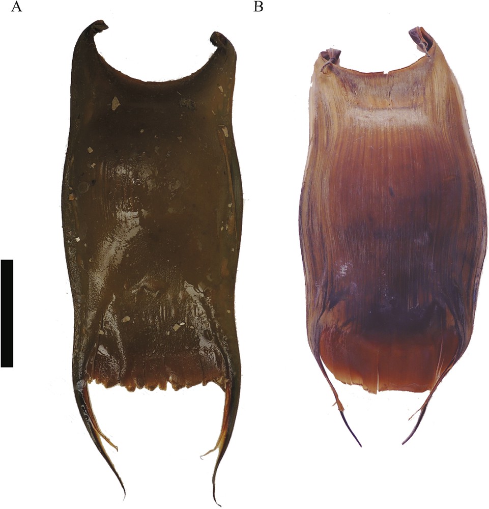
The morphological and molecular comparisons between specimens of Z. chilensis from SEP and from SWA, presented here, revealed that they correspond to different nominal species. Zearaja chilensis (Guichenot, 1848) was described for the first time under the name R. chilensis by Guichenot in 1848 [72]. In 1892, Philippi described R. flavirostris based on two female specimens, and R. oxyptera from an adult male found in Quinteros bay, Chile and declared not having found R. chilensis [73]. Delfin [74] described Raja latastei based on the analysis of a male and a female collected in La Herradura, Coquimbo, Chile. He regarded R. latastei as a different species from that described by Philippi. Garman [75] regarded R. oxyptera as a junior synonym of R. flavirostris, suggesting that the morphological differences between the two nominal species have been attributed to age and sex, and he also included R. latastei Delfin 1902 in the synonymy. In 1928, Marini reported the occurrence of Raja stabuliforis (= Dipturus laevis) in Argentine waters, based on specimens collected off the Buenos Aires coast [76]. Five years later, the author made an amendment about this record based on comparison with the type material and described Raia brevicaudata as a new longnose skate species [77]. Norman [10] later gave a description of specimens from Argentine waters and synonymized R. brevicaudata to R. flavirostris. It is noteworthy that Norman stated, when he gave the detailed description of Raja flavirostris: “I received a specimen of R. brevicaudata from Buenos Aires (Marini) […] I have been unable to examine any Chilean material of this long-snouted form, but have little doubt that the specimens described here are identical with the large male and female described by Philippi as R. oxyptera and R. flavirostris respectively.” Since Norman [10], the work of Marini has faded into oblivion and nobody was raised to compare specimens from both oceans, until now. As happened in other recent cases [78,79], molecular evidence led to reconsider taxonomic issues. Given that Z. chilensis and Z. flavirostris were first used in the description of Chilean specimens by Guichenot [72] and Philippi [73], respectively, it is necessary to rename the specimens from SWA. Looking for available names in the literature, Marini [77] was the first who described longnose skates from these waters. Based on clasper morphology, the resurrected species is tentatively included (see discussion) in the Genus Zearaja. Therefore, the suitable name for the species is Z. brevicaudata and is resurrected herein. The holotype of Z. brevicaudata (Fig. 8) was included in the analyses and was placed with the Argentine specimens (Figs. 2–3); its measurements are given in Table 4. It would have been important and enriching for the purpose of the work to analyze the type material of R. chilensis Guichenot 1848 and R. flavirostris Philippi 1892. But unfortunately, this material does not exist.

Fig. 8
Holotype of Zearaja brevicaudata (Marini 1933) in dorsal (A) and ventral view (B). The black bar represents 50 mm.

Table 4

	Holotype
Total length	324
Disc width	250
Direct disc length	200
Indirect disc length	197
Snout to maximum width	122
Direct preorbital length	62
Indirect preorbital length	60.4
Snout to spiracle	81.5
Dorsal head length	84.42
Orbit diameter	14.6
Orbit and spiracle length	18.7
Spiracle length	7.4
Distance between orbits	16.13
Distance between spiracles	25.11
Snout to cloaca	183
Tail length (cloaca to caudal-fin tip)	140.32
Ventral snout length (preoral)	64.2
Direct prenasal length	60.7
Indirect prenasal length	58
Direct ventral head length	110.44
Indirect ventral head length	109
Mouth width	30.6
Distance between nostrils	30.4
Nasal curtain length	13.3
Nasal curtain total width	31.4
Width of first gill opening	4.52
Width of fifth gill opening	5.01
Distance between first gill openings	53.5
Distance between first gill openings	34.04
Length of anterior pelvic lobe	42.7
Length of posterior pelvic lobe	49
Pelvic base width	38.11
Tail width at axis of pelvic fin	13.5
Tail height at axis of pelvic fin	13.2
Tail width at tail midlength	7.6
Tail height at tail midlength	5.3
Tail width at D1 origin	9.1
Tail height at D1 origin	4.7
D1 base length	18.3
D1 height	11.4
D1 origin to caudal tip	55.6
D2 origin to caudal tip	33.4
Caudal-fin length	13.2
Caudal-fin height	2.7

4.1 Previous references

Raia stabuliforis:[76] [misidentification], Raia brevicaudata [77], Raja flavirostris: [10,80–82], Raja (Dipturus) flavirostris: [39,43,44], Dipturus flavirostris: [12], Dipturus chilensis: [15,77,83–87], Zearaja chilensis: [5] [in part]; [35] [in part]; [47,66,88], Zearaja flavirostris: [49,52,89].

4.2 Diagnosis

Zearaja brevicaudata is a relatively large species of skate with a rhombic-shaped disc characterized by the combination of the following characters: relatively large snout (1.7–2.9 times tail length), short tail (2.1–2.7 times in total length), and short distance between the first gill openings (3.42–4.19 times indirect disc length). Even though these relationships overlap with those of Z. chilensis, these features differ diagnostically among specimens of similar size (Fig. 7). The dermal denticles are mainly restricted to the rostral area, both in dorsal and ventral surfaces. Denticles are more conspicuous in adults, and can be absent or in less number in neonates and juveniles. Three to five rows of thorns are present on the tail (rarely only one). The clasper is relatively long and stout, 74–78% of the tail's length in adult specimens. The terminal bridge (Tb) is straight towards the tip of dorsal terminal 2, and the spike is thin and does not reach the Tb. The ventral terminal cartilage has a short apophysis, and its outer edge is narrow. The distal tip of the axial is relatively narrow.

Fig. 7
Direct relation between total length (LT) and preorbital indirect length (PorbL) (A), preoral length (PorL) (B), distance between first gill openings (DG1) (C) and tail length (TaL)(D) of specimens of Zearaja brevicaudata (triangles) andZearaja chilensis (circles). All measurements are given in mm.

4.3 Redescription of the holotype

MACN Ict-569, Atlantic Coast of Buenos Aires, Cap Alexandersson, vapor “Maneco” (Fig. 8). A juvenile female of 324 mm TL and 250 mm disc width with a relatively large snout (ventral snout length 2.2 times tail length, 5.1 in total length), a short tail (2.3 times in total length), and a short distance between the first gill openings (3.7 times indirect disc length). The disc is broader than long (disc width 1.25 times disc length). The mouth is as wide as half (0.47) of the snout length. Teeth number on the upper jaw: 35. Distance between orbits: 1.1 times the orbit diameter. Dorsal surface smooth with no denticles perceived to the touch. A well-developed thorn on the snout tip and two on the anterior margin of each pectoral fin. Four ocular thorns around each eye and one nuchal thorn are present. No spiracular thorns. Three rows of caudal thorns: mid-caudal line with twelve thorns and one interdorsal thorn, lateral rows with four thorns each. Surface of the dorsal fins slightly rough in the anterior margin. Ventral surface smooth with denticles only in the anterior margin of the snout and on the tip of the rostral process. The ventral surface of the tail is smooth. No thorns are present on the ventral surface. The morphometric values are shown in Table 4.

4.4 Distribution

Endemic of the Southwestern Atlantic, from southern Brazil to at least the Beagle Channel. It inhabits between 25–350 m in depth, with the highest abundance between 50 and150 m. It also occurs in San Matias and San Jorge Gulfs [90].

4.5 Common names

In English: “Yellownose skate” is used for both Z. chilensis and Z. brevicaudata, therefore we suggest the name “short tail Yellownose skate”. In Spanish: Raya hocicuda de cola corta.

5 Discussion

Zearaja brevicaudata is resurrected herein, based on an integrative comparison between Argentinian and Chilean specimens identified as Z. chilensis, which included: classical morphology and morphometric analyses, spinulation and denticle pattern, clasper morphology, egg case morphology, and molecular analysis. Last and Gledhill [47] resurrected the genus Zearaja mainly based on clasper morphology, and provided a detailed comparison of the claspers of Zearaja and Dipturus. The authors also included D. chilensis within the genus Zearaja based on its clasper morphology. However, Naylor et al. [49] have called into question the validity of the genus based on molecular data. Specifically, the authors stated that the genus Dipturus would be monophyletic only if the genus Zearaja was included within Dipturus. Given that no new phylogenetic results were presented since 2012, the query was not fully resolved yet, and therefore the resurrected species was included tentatively within the genus Zearaja.

Differences in external morphology, pattern of spinulation, clasper and egg cases morphology, allowed distinguishing Z. brevicaudata from Z. chilensis. The characteristics observed herein for Z. chilensis were consistent with those reported by Leible [91], who analyzed a large number of juvenile and adult specimens of Z. chilensis (as Raja (Dipturus) flavirostris) from SEP. Indeed, the range values of the most important feature that distinguish both species (the distance between first-gill openings) obtained by this author was 18–22.3%, out of the range of Z. brevicaudata (less than 18%). Leible [91] remarked that specimens from Chilean waters presented shorter snout than those from Argentinian waters, based on the results of Menni [43]. Even though, these relationships overlap with those of Z. chilensis (as was previously reported), these variables differed diagnostically among specimens of equal size, having Z. brevicaudata longer snout and shorter distance between the first gill openings than Z. chilensis.

Leible [91] described the clasper of Z. chilensis, remarking on the internal and external components. However, no detailed description of the size and shape of each component was provided beyond the pictures. Menni [65] described the inner components of the clasper of Z. brevicaudata (as Raja (Dipturus) flavirostris), based on SWA specimens, and indicated an accessory terminal 1(At1). However, in the present study, cartilages of Z. brevicaudata were disarticulated and it was found that the piece considered by Menni [65] as At1 is actually part of the Dm. Therefore, At1 is absent in the clasper of Z. brevicaudata. This is consistent with the observations of Leible [91] and Last and Gledhill [47] for specimens of Zearaja. Terminal series cartilages are known to be species-specific on skates [1,46,62,92–94]. Herein, even sharing the same external and internal components, differences on the shape of several cartilages were observed between the claspers of Z. brevicaudata and Z. chilensis, allowing us to differentiate them.

Egg-cases morphology is also species-specific [66,95–99]. Egg cases of Z. brevicaudata have a thinner lateral keel than those of Z. chilensis. Differences in egg-case length were noticed previously by Concha et al. [99], who stated that both length and width ranges of egg cases were considerably smaller in the South West Pacific. The range values of egg case length and egg case maximum width for Z. brevicaudata were 115–158 mm and 58.7–70.8 mm, respectively. Those of Z. chilensis were 94–144 mm and 64–76 mm [99]. Unfortunately, only two egg cases from Chilean waters could be analyzed; therefore, the ranges given here for Z. chilensis do not include the entire variation the species may present.

Five nominal species of longnose skates have been recorded in the South West Atlantic Ocean, from southern Brazil to southern Argentina. Coloration pattern and tail distinguish Z. brevicaudata from D. argentinensis. The dorsal surface of the disc of Z. brevicaudata is grayish, with an ocellus on each pectoral fin and pale fuzzy circles scattered over the entire dorsal surface; the ventral surface is whitish with gray blotches; the snout is translucent and both sides of the rostrum are yellowish-white; the tail is short and wide, with 3–5 thorn rows. The tail length is 41% of the body length, and its width is 10% of the tail length. On the other hand, the ventral surface of the disc of D. argentinensis is as dark as the dorsal surface, the snout is not translucent, the tail is rather long (47% of the body length) and slender (7.5% of the tail length) with one row of caudal thorns [78]. Zearaja brevicaudata differs from D. trachyderma by the denticle and spinulation patterns. The former presents both surfaces of snout covered by denticles and the rest of disc is smooth; ocular and nuchal thorns are present. Conversely, dorsal and ventral surface of disc of D. trachyderma are thornless but densely covered with coarse denticles [63]. Zearaja brevicaudata distinguishes from D. mennii by its smooth interorbital space and the absence of thorn row from the nuchal region to the beginning of the tail. In contrast, D. mennii presents a continuous row of thorns from the nuchal region to the first-dorsal fin and an interorbital region covered with coarse denticles [100]. Zearaja brevicaudata has no suprascapular thorn, its mouth width is two times in preoral length, and the occurrence of fuzzy pale circles distinguishes it from D. leptocauda. The latter species presents two suprascapular thorns, a mouth width that is three times in preoral length, a dorsal surface of the disc with dark brown color with numerous rounded pale whitish blotches and a remarkable thin tail [101].

There are two different commercial markets for the skates. One of them is the European market, in which the fins are sold without preference of any species. The other one is the Asian market, which has preference for Z. brevicaudata and Z. chilensis, known as the red skate or longnose skate [31]. Due to the increasing demand on these international markets, the fishing pressure on all skates has increased since 1994 in the shelf waters of Argentina, rising from 761 tons in 1992 to a maximum of 26,957 tons in 2008 [102]. In the direct fishing of Z. brevicaudata, onboard observation showed that in 2000 and 2001, a longline vessel fished from 37° to 44°S off Argentina, between 50 and 100 m in depth. The species accounted for more than 50% of the total skate's catch, and 30% of the captured individuals corresponded to juveniles [29]. Zearaja brevicaudata is also taken as bycatch in the fisheries that operate in the South West Atlantic. In Puerto Quequén (Buenos Aires province), Z. brevicaudata is fished as bycatch in the target fisheries of Zidona dufresnei (Neogastropoda: Volutidae), flatfishes (Osteichthyes: Paralichthyidae) and the smoothound Mustelus schmitti (Chondrichthyes: Triakidae) [103]. Estalles et al. [21] found that Z. brevicaudata was one of the most abundant species in the analyzed skate landings as bycatch of fisheries of the common hake in the San Matias Gulf. This longnose skate was recorded in all landings and more of the 80% of the individuals collected were smaller than 600 mm. Even in this study, 93% of the analyzed individuals from fisheries corresponded to juveniles. Due to the high levels of exploitation, Z. brevicaudata (listed as Z. chilensis) is categorized as vulnerable species by the IUCN. Paesch and Oddone [19] estimated the LT₅₀ (length at which half of the individuals in the population are sexually mature) of 78.5 cm for males and 81.4 cm for females, from specimens collected in the Argentinean–Uruguayan Common Fishing Zone. Colonello and Cortes [104] found values of LT₅₀ of 78 cm and 90.8 for males and females, respectively from specimens collected in the entire species distribution range. This information must be taken into account to create management policies that protect the species, given that the survival of juveniles is a key factor for the maintenance of populations of elasmobranch fishes [7]. Since specimens currently known as Z. chilensis from the Pacific and Atlantic Oceans actually correspond to different species, caution must be taken with previous information regarding biological parameters. Therefore, a new IUCN assessment should be performed for each species. Given its endemism and the importance of this species in Southwestern Atlantic fisheries, further research and a continuous monitoring that allow assessing the abundance, geographic range distribution and population status of Z. brevicaudata are urgently needed.

Funding

This work was supported by CONICET (PIP No. 11220130100339), MINCYT (PICT-2014-0665) and Universidad Nacional de Mar del Plata (EXA 867/18).

Disclosure of interest

The authors declare that they have no competing interest.

Acknowledgments

This research is part of Gabbanelli V. PhD Universidad de Mar del Plata and CONICET scholarship. We thank Mariano Gulielmetti, Santiago Barbini, David Sabadin and Solimeno S. A., for providing some of the samples in Argentina. We thank Francisco Concha for providing samples from Chile. We wish to thank the crew of the A.R.A Puerto Deseado for helping in the collection of samples. We would like to thank Gustavo Chiaramonte for receiving us at the “Museo Argentino de Ciencias Naturales Bernardino Rivadavia”, and Augusto Cornejo, Jhoann Canto and Herman Núñez for receiving us and the good treatment they gave us at the Museo Nacional de Historia Natural de Chile. We thank Matías Delpiani for contributing with DNA extraction and PCR amplification process. Finally, we thank Damian Castellini, Mariana Deli Antoni, Cecilia Spath and Gabriela Delpiani for helping in the measurement process. Finally, we would like to thank two anonymous reviewers for offering helpful comments that improved the earlier draft of the manuscript.

References

[1] J.D. McEachran; T. Miyake Zoogeographic and bathymetry of skates (Chondricthyes. Rajoidei) (H.L. Pratt; S.H. Gruber; T. Taniuchi, eds.), Elasmobranchs as living resources: advances in the biology, Ecology, systematic, and the status of the fisherie, United States National Marine Fisheries Service, NOAA Technical Report, 1990, pp. 305-326

[2] D.A. Ebert; L.J.V. Compagno Biodiversity and systematics of skates (Chondrichthyes: Rajiformes: Rajoidei), Environ. Biol. Fish., Volume 80 (2007), pp. 111-124 | DOI

[3] P.R. Last New short-snout members of the skate genus Dipturus (Rajoidei: Rajidae) from Australian seas (P.R. Last; W.T. White; J.J. Pogonoski; D.C. Gledhill, eds.), Descriptions of New Australian Skates (Batoidea: Rajoidei), CSIRO Marine & Atmospheric Research, Canberra, 2008, pp. 53-98

[4] L.J.V. Compagno; D.A. Ebert; M.J. Smale Guide to the sharks and rays of southern Africa, Struik Publishers, Cape Town, 1989

[5] P.R. Last; S. Weigmann; L. Yang Changes to the nomenclature of the skates (Chondrichthyes: Rajiformes) (P.R. Last; G.K. Yearsley, eds.), Rays of the World: Supplementary information, CSIRO Special Publication, Canberra, 2016, pp. 11-34

[6] M.G. Frisk; T.J. Miller; M.J. Forgarty Estimation and analysis of biological parameters in elasmobranch fishes: a comparative life history study, Can. J. Fish. Aquat. Sci., Volume 58 (2001), pp. 969-981 | DOI

[7] J.D. Stevens; R. Bonfil; N.K. Dulvy; P.A. Walker The effects of fishing on shark, Rays, and chimaeras (Chondrichthyans), and the implications for marine ecosystems, ICES J. Mar. Sci., Volume 57 (2000), pp. 476-494 | DOI

[8] N.K. Dulvy; S.L. Fowler; J.A. Musick; R.D. Cavanagh; P.M.L. Kyne; R. Harrison; J.K. Carlson; L.N.K. Davidson; S.V. Fordham; M.P. Francis; C.M. Pollock; C.A. Simpfendorfer; G.H. Burgess; K.E. Carpenter; L.J.V. Compagno; D.A. Ebert; C. Gibson; M.R. Heupel; S.R. Livingstone; J.C. Sanciangco; J.D. Stevens; S. Valenti; W.T. White Extinction risk and conservation of the world's sharks and rays, eLife, Volume 3 (2014), p. e00590 | DOI

[9] P.R. Last; W.T. White; M.R. de Carvalho; B. Séret; M.F.W. Stehmann; G.J.P. Naylor Rays of the World, CSIRO Publishing, Australia, 2016

[10] J.R. Norman Coast fishes Part II: The Patagonian region, Discov. Rep., Volume 16 (1937), pp. 1-150

[11] D.J. Agnew; C.P. Nolan; J.R. Beddington; R. Baranowski Approaches to the assessment and management of multispecies skate and ray fisheries using the Falkland Islands fishery as an example, Can. J. Fish. Aquat. Sci., Volume 57 (2000), pp. 429-440 | DOI

[12] R.C. Menni; M.F. Stehmann Distribution, environment and biology of batoid fishes off Argentina, Uruguay and Brazil. A review, Rev. Mus. Argentino. Cienc. Nat., Volume 2 (2000), pp. 69-109

[13] U.L. Gomes; S. Picado Distribution of the species of Dipturus Rafinesque (Rajidae, Rajinae, Rajini) off Brazil and first record of the Caribbean skate D. teevani (Bigelow & Schroeder). in the Western South Atlantic, Rev Bras Zool., Volume 18 (2001), pp. 171-185 | DOI

[14] C. Bustamante; C. Vargas-Caro; M.B. Bennett Not all fish are equal: functional biodiversity of cartilaginous fishes (Elasmobranchii and Holocephali) in Chile, J. Fish. Biol., Volume 85 (2014), pp. 1617-1633 | DOI

[15] M.B. Cousseau; D.E. Figueroa; J.M. Díaz de Astarloa; E. Mabragaña; L.O. Lucifora Rayas, chuchos y otros batoideos del Atlántico Sudoccidental (34° S–55° S), Instituto Nacional de Investigación y Desarrollo Pesquero (INIDEP), Mar del Plata, Argentina, 2007

[16] M. Fuentealba; M. Leible Perspectivas de la pesquería de la raya volantín Raja (Dipturus) flavirostris. Estudio de edad, crecimiento y algunos aspectos reproductivos (M.A. Barbieri, ed.), Perspectivas de la actividad pesquera en Chile, Universidad Católica de Valparaíso, Valparaíso, Chile, 1990, pp. 227-236

[17] R. Licandeo; J. Lamilla; P.G. Rubilar; R. Vega Age, Growth, and sexual maturity of the yellownose skateDipturus chilensis in the south-eastern Pacific, J. Fish. Biol, Volume 68 (2006), pp. 488-506 | DOI

[18] R. Licandeo; F.T. Cerna Geographic variation in life- history traits of the endemic kite skate Dipturus chilensis (Batoidea: Rajidae), along its distribution in the fjords and channels of southern Chile, J. Fish. Biol., Volume 71 (2007), pp. 421-440 | DOI

[19] L. Paesch; M.C. Oddone Change in size-at-maturity of the yellownose skate Dipturus chilensis (Guichenot. 1848) (Elasmobranchii: Rajidae) in the SW Atlantic, Neotrop. Ichthyol., Volume 6 (2008), pp. 223-230 | DOI

[20] M.I. Aversa; S.L. Dans; N.A. García; E.A. Crespo Growth models fitted to Dipturus chilensis length-at-age data support a two-phase growth, Rev. Chil. Hist. Nat., Volume 84 (2011), pp. 33-49 | DOI

[21] M. Estalles; N.M. Coller; M.R. Perier; E.E. Di Giácomo Skates in the demersal trowl fishery of San Matías Gulf, Patagonia: species composition, relative abundance and maturity stages, Aquat. Living Resour., Volume 24 (2011), pp. 193-199 | DOI

[22] C. Bustamante; C. Vargas-Caro; M.C. Oddone; F. Concha; H. Flores; J. Lamilla; M. Bennett Reproductive biology of Zearaja chilensis (Guichenot, 1848) (Chondrichthyes: Rajidae) in the southeast Pacific Ocean, J. Fish. Biol., Volume 80 (2012), pp. 1213-1226 | DOI

[23] M. Koen Alonso; E.A. Crespo; N.A. García; S.N. Pedraza; P.A. Mariotti Food habits of Dipturus chilensis (Pisces: Rajidae) off Patagonia, Argentina, ICES J. Mar. Sci., Volume 58 (2001), pp. 288-297 | DOI

[24] M. Belleggia; N. Andrada; S. Paglieri; F. Cortés; A.M. Massa; D.E. Figueroa; C. Bremec Trophic ecology of yellownose skate Zearaja chilensis, a top predator in the south-western Atlantic Ocean, J. Fish. Biol., Volume 88 (2016), pp. 1070-1087 | DOI

[25] R. Roa; B. Ernst Informe Final del Proyecto Investigación CTP de raya volantín entre la VIII y X Regiones, Subsecretaría de Pesca, Chile, 1999

[26] R. Roa; B. Ernst Informe Final del Proyecto Investigación CTP de raya volantín entre la VIII y X Regiones, Subsecretaría de Pesca, Chile, 2000

[27] J. Lamilla; R. Roa; P. Barría; C. Bustamante; F. Concha; E. Cortes; E. Acuña; F. Balbontín; M. Oliva; M. Araya; R. Meléndez Desarrollo metodológico para la estimación del descarte de Condrictios en las pesquerías artesanales. Informe Final Proyecto del Fondo de Investigación Pesquera (F.I.P.) No. 2006-31, Subsecretaría de Pesca, Universidad Austral de Chile, Chile, 2008

[28] J. Lamilla; C. Bustamante; R. Roa; E. Acuña; F. Concha; R. Meléndez; S. López; G. Aedo; H. Flores; C. Vargas-Caro Estimación del descarte de condrictios en pesquerías artesanales Informe Final Proyecto del Fondo de Investigación Pesquera (F.I.P.) No. 2008-60, Subsecretaría de Pesca, Universidad Austral de Chile, Chile, 2010

[29] J.H. Colonello; A.M. Massa; L.O. Lucifora Composición de la captura de rayas del buque palangrero “Sureste 501” en el norte del Mar Argentino, INIDEP Inf. Téc., Volume 107 (2002), pp. 1-13

[30] A.M. Massa; N.M. Hozbor; J.H. Colonello Situación actual y avances en el estudio de los peces cartilaginosos, INIDEP Inf. Téc., Volume 57 (2004), pp. 1-18

[31] A.M. Massa; L.O. Lucifora; N.M. Hozbor Condrictios de las regiones costeras Bonaerense y Uruguaya (R. Sánchez; S. Bessi, eds.), El Mar Argentino y Sus Recursos Pesqueros. Tomo 4. Los Peces Marinos de Interés Pesquero. Caracterización Biológica y Evaluación del Estado de Explotación INIDEP, Mar del Plata, 2004, pp. 85-99

[32] P.V. Cedrola; A.M. González; A.D. Pettovello Bycatch of skates (Elasmobranchii: Arhynchobatidae, Rajidae) in the Patagonian red shrimp fishery, Fish. Res., Volume 71 (2005), pp. 141-150 | DOI

[33] R.C. Wakeford; D.J. Agnew; D.A.J. Middleton; J.H.W. Pompert; V.V. Laptikhovsky Management of the Falkland Islands Multispecies ray fishery: Is species specific management required?, J. Northwest Atl. Fish. Sci., Volume 37 (2004), pp. 309-324 | DOI

[34] P.M. Kyne; J. Lamilla; R.R. Licandeo; J. San Martín; M. Stehmann; C. McCormack Zearaja chilensis, The IUCN Red List of Threatened Species 2007: e. T63147A12623314, 2007 ([http:dx.doi.org/10.2305/IUCN.UK.2007.RLTS.T63147A12623314.en ; Accessed on 07 February 2018])

[35] C. Vargas-Caro; C. Bustamante; J. Lamilla; M.B. Bennett A review of longnose skates Zearaja chilensis and Dipturus trachyderma (Rajiformes: Rajidae), Univ. Sci., Volume 20 (2015), pp. 321-359 | DOI

[36] F. De Buen Tiburones, rayas y quimeras en la Estación de Biología Marina de Montemar, Chile, Rev. Biol. Mar., Volume 10 (1959), pp. 1-50

[37] G. Pequeño; J. Lamilla Estudio sobre una colección de rayas del sur de Chile (Chondrichthyes, Rajidae), Rev. Biol. Mar., Volume 21 (1985), pp. 225-271

[38] G. Pequeño Peces de Chile, Rev. Biol. Mar. Oceanogr., Volume 24 (1989), pp. 1-132

[39] D. Lloris; J. Rucabado Ictiofauna del Canal Beagle (Tierra de Fuego): aspectos ecológicos y análisis biogeográfico, Pub Esp IEO., Volume 8 (1991), pp. 1-182

[40] G. Pequeño; J. Lamilla Batoideos comunes a las costas de Chile y Argentina-Uruguay (Pisces: Chondrichthyes), Rev. Biol. Mar. Oceanogr., Volume 28 (1993), pp. 203-217

[41] S. Sáez; J. Lamilla Morfología y disposición de los dientes en una especie con heterodontía sexual: Raja (Dipturus) chilensis Guichenot, 1848, Biol. Pesq., Volume 26 (1997), pp. 25-41

[42] M. Stehmann Vergleichend morphologische und anatomische untersuchungen zur Neuordnung der Systematik der nordostatlantischen Rajidae (Chondrichthyes, Batoidei), Arch. Fischereiwiss., Volume 21 (1970) no. 2, pp. 73-164

[43] R.C. Menni Rajidae del litoral bonaerense. I Especies de los géneros Raja. Bathyraja y Sympterygia (Chondrichthyes), Physis, Volume 32 (1973), pp. 413-439

[44] R.C. Menni; R.A. Ringuelet; R.H. Arámburu Peces marinos de la Argentina y Uruguay. Reseña histórica. Clave de familias, géneros y especies, Catálogo crítico, Hemisferio Sur, Buenos Aires, 1984

[45] H.L. López; M.L. García; N.A. San Román Ictiofauna del Canal Beagle (Sector Argentino), Neotropica, Volume 35 (1989), pp. 1-50

[46] J.D. McEachran; K.A. Dunn Phylogenetic analysis of skates, a morphologically conservative clade of elasmobranchs (Chondrichthyes: Rajidae), Copeia, Volume 2 (1998), pp. 271-290

[47] P.R. Last; D. Gledhill The Maugean skate, Zearaja maugeana sp. nov. (Rajiformes: Rajidae)–a micro endemic Gondwanan relict from Tasmanian estuaries, Zootaxa, Volume 1494 (2007), pp. 45-65

[48] W.N. Eschmeyer Catalog of fishes. Special Publication (3 vols.), Academy of Sciences San Francisco, California, 1998

[49] G.J.P. Naylor; J.N. Caira; K. Jensen; K.A.M. Rosana; W.T. White; P.R. Last A DNA sequence-based approach to the identification of sharks and ray species and its implications for global elasmobranch diversity and parasitology, Bull. Am. Mus. Nat. Hist., Volume 367 (2012), pp. 1-262 | DOI

[50] D. Jeong; Y.H. Lee Complete mitochondrial genome of the yellownose skate: Zearaja chilensis (Rajiformes. Rajidae), Mitochondr. DNA, Volume 27 (2014) no. 1, pp. 293-294 | DOI

[51] C. Vargas-Caro; C. Bustamante; M.B. Bennett; J.R. Ovenden The complete validated mitochondrial genome of the yellownose skate Zearaja chilensis (Guichenoti 1848) (Rajiformes. Rajidae), Mitochondr. DNA, Volume 27 (2014) no. 2, pp. 1227-1228 | DOI

[52] S. Izzo; G. Andreoli; D.E. Figueroa; M. Costagliola Molecular characterization of sympatric skates of the Dipturus and Zearaja genera of the Argentine Sea with DNA Barcode, Rev. Invest. Desarr. Pesq., Volume 31 (2017), pp. 55-74

[53] P.R. Last; W.T. White; J.J. Pogonoski; D.C. Gledhill New Australian skates (Batoidea: Rajoidei) – background and methodology (P.R. Last; W.T. White; J.J. Pogonoski; D.C. Gledhill, eds.), Description of new Australian skates (Batoidea: Rajoidei), CSIRO Marine and Atmospheric Research, Canberra, 2008, pp. 1-8

[54] J. Lleonart; J. Salat; G.J. Torres Removing allometrics effects of body size in morphological analysis, J. Theor. Biol., Volume 205 (2000), pp. 85-93 | DOI

[55] A. Lombarte; J. Lleonart Otolith size changes related with body growth, habitat depth and temperature, Environ. Biol. Fish., Volume 37 (1993), pp. 297-306

[56] M. González-Castro; J.J. Rosso; E. Mabragaña; J.M. Díaz de Astarloa Surfing among species, populations and morphotypes: inferring boundaries between two species of new world silversides (Atherinopsidae), C. R. Biologies, Volume 399 (2016) no. 1, pp. 10-29 | DOI

[57] P. Orlando; M. González-Castro; E. Mabragaña New insights to discriminate between Sympterygia acuta Garman 1877 and Sympterygia bonapartii Muller & Henle, 1841 (Rajidae) of the Southwest Atlantic Ocean: On the use of geometric morphometrics and spinulation patterns, J. Appl. Ichthyol., Volume 31 (2015), pp. 381-389 | DOI

[58] D. Sabadin; M. González Castro; C. Iudica; J.M. Díaz de Astarloa; P.J. Fernández Iriarte Morphometric and genetic assessment of the Cynoscion guatucupa population structure from Buenos Aires coast, Argentine sea, Rev. Biol. Mar. Oceanogr., Volume 45 (2010) no. 3, pp. 513-517

[59] R. Salomón; S. Melo; N. Winzer MULTIVARIADO software. Departamento de Matemática, Universidad Nacional del Sur, Argentina, 2004

[60] K.R. Clarke; R.M. Warwick Changes in marine communities: an approach to statistical analysis and interpretation, PRIMER-E: Plymouth Marine Laboratory, United Kingdom, 2001

[61] R. Gravendeel; W. Van Neer; D. Brinkhuizen An identification key for dermal denticles of Rajidae from the North Sea, Int. J. Osteoarchaeol., Volume 12 (2002), pp. 420-441 | DOI

[62] P. Hulley The origin, interrelationships and distribution of southern African Rajidae (Chondricthyes, Batoidei), Ann. S. Afr. Mus., Volume 60 (1972) no. 1, pp. 1-103

[63] M.D. Leible; M. Stehmann First records of Raja (Dipturus) trachyderma Krefft & Stehmann, 1975 from the southeastern Pacific off Chile, with first descriptions of its clasper characters and additional skeletal and morphological details (Pisces, Rajiformes, Rajidae), Stud. Neotrop. Fauna E., Volume 22 (1987), pp. 169-188 | DOI

[64] M.D. Leible Revisión de métodos taxonómicos para el estudio de rayas (Rajiformes. Rajidae), Gayana, Zoologia, Volume 52 (1988) no. 1–2, pp. 15-93

[65] R.C. Menni Anatomia del mixopterigio y posición sistemática deRaja flavirostris Philippi, 1892, Neotropica, Volume 17 (1971) no. 52, pp. 39-43

[66] E. Mabragaña; D.E. Figueroa; L.B. Scenna; J.M. Díaz de Astarloa; J.H. Colonello; G. Delpiani Chondrichthyan egg cases from the south-west Atlantic Ocean, J. Fish. Biol., Volume 79 (2011), pp. 1261-1290

[67] N.V. Ivanova; J.R. deWaard; P.D.N. Hebert An inexpensive, automation-friendly protocol for recovering high-quality DNA, Mol. Ecol. Notes., Volume 6 (2006), pp. 998-1002 | DOI

[68] N.V. Ivanova; T.S. Zemlak; R.H. Hanner; P.D.N. Hebert Universal primer cocktails for fish DNA barcoding, Mol. Ecol. Notes, Volume 7 (2007), pp. 544-548 | DOI

[69] K. Tamura; G. Stecher; D. Peterson; A. Filipski; S. Kumar MEGA6: Molecular Evolutionary Genetics Analysis Version 6.0, Mol. Biol. Evol., Volume 30 (2013), pp. 2725-2729 | DOI

[70] M. Kimura A simple method for estimating evolutionary rate of base substitutions through comparative studies of nucleotide sequences, J. Mol. Evol., Volume 16 (1980), pp. 111-120

[71] S. Ratnasingham; P.D.N. Hebert DNA-based registry for all animal species: the barcode index number (BIN) system, PLoS ONE, Volume 8 (2013), p. 8e66213

[72] A. Guichenot Fauna Chilena. Peces (C. Gay, ed.), Historia física y política de Chile II, Museo de Historia Natural de Chile, Santiago, 1848, pp. 137-370

[73] R.A. Philippi Algunos peces de Chile: Las rayas. Callorhynchus i Orthagoriscus chilenos, Anales del. Mus. Nac. Santiago de Chile, Volume 3 (1892), pp. 1-16

[74] F.T. Delfin Nuevas Especies de la Familia Rajidae, Rev. Chil. Hist. Nat., Volume 6 (1902), pp. 262-270

[75] S. Garman The Plagiostomia (sharks. skates and rays), MCZ Memoirs, Volume 36 (1913), pp. 1-528 | DOI

[76] T.L. Marini Nota sobre dos rayas nuevas para la costa atlántica de la provincia de Buenos Aires, Physis, Volume 9 (1928), pp. 133-141

[77] T.L. Marini Rectificando errores ictiológicos, Physis, Volume 11 (1933), pp. 328-332

[78] J.M. Díaz de Astarloa; E. Mabragaña; R. Hanner; D.E. Figueroa Morphological and molecular evidence for a new species of longnose skate (Rajiformes: Rajidae: Dipturus) from Argentinian waters based on DNA barcoding, Zootaxa, Volume 1921 (2008), pp. 35-46

[79] P.R. Last; B. Séret A new Eastern Central Atlantic skate Raja parva sp. nov. (Rajoidei: Rajidae) belonging to the Raja miraletus species complex, Zootaxa, Volume 4147 (2016) no. 4, pp. 477-489 | DOI

[80] R.A. Ringuelet; R.H. Aramburu Sistemática y biología de los peces marinos de la plataforma continental Argentina, Boletin -Ministerio de Asuntos Agrarios Direccion de Recursos Pesqueros, Volume 12 (1971), pp. 5-16

[81] R.C. Menni; H.L. López Distributional patterns of Argentine marine fishes, Physis, Volume 42 (1984), pp. 71-85

[82] S.B. García de La Rosa Estudio de la interrelaciones tróficas de dos elasmobranquios del Mar Argentino, en relación con las variaciones espacio-temporales y ambientales Squalus acanthias (Squalidae) y Raja flavirostris (Rajidae), Universidad Nacional de Mar del Plata, Mar del Plata, 1998

[83] M.B. Cousseau; D.E. Figueroa; J.M. Díaz de Astarloa Clave de identificación de las rayas del litoral marítimo de Argentina y Uruguay (Chondrichthyes, Familia Rajidae), Instituto Nacional de Investigación y Desarrollo Pesquero (INIDEP), Mar del Plata, 2000

[84] L.O. Lucifora; J.L. Valero; C.S. Bremec; M.L. Lasta Feeding habits and prey selection by the skate Dipturus chilensis (Elasmobranchii: Rajidae) from the south-western Atlantic, J. Mar. Biol. Assoc. UK, Volume 80 (2000), pp. 953-954

[85] F. Sánchez; E. Mabragaña Características biológicas de algunas rayas de la región sud Patagónica, INIDEP Inf. Téc., Volume 48 (2002), pp. 1-15

[86] S.B. García de la Rosa; F. Sánchez; L.B. Prenski Caracterización biológica y estado de explotación de la raya (Dipturus chilensis) (R.P. Sánchez; S.I. Bezzi, eds.), El Mar Argentino y sus recursos pesqueros Tomo 4. Los peces marinos de interés pesquero: Caracterización biológica y evaluación del estado de explotación, Publicaciones Especiales INIDEP, Mar del Plata, 2004, pp. 53-66

[87] M.C. Oddone; L. Paesch; W. Norbis Size at first sexual maturity of two species of rajoid skates, genera Atlantoraja and Dipturus (Pisces, Elasmobranchii, Rajidae), from the south-western Atlantic Ocean, J. Appl. Ichthyol., Volume 21 (2005), pp. 70-72 | DOI

[88] M.Y. Deli Antoni; G.E. Delpiani; S.M. Delpiani; E. Mabragaña; J.M. Díaz de Astarloa An aberrant extra fin in Zearaja chilensis (Chondrichthyes: Rajidae), Cybium, Volume 36 (2012), pp. 403-405

[89] R.C. Menni; A.J. Jaureguizar; M.F. Stehmann; L.O. Lucifora Marine biodiversity at the community level: zoogeography of sharks, skates, rays and chimaeras in the southwestern Atlantic, Biodivers. Conserv., Volume 19 (2010), pp. 775-796 | DOI

[90] M.B. Cousseau; R.G. Perrotta Peces marinos de Argentina: biología, distribución, pesca, Instituto Nacional de Investigación y Desarrollo Pesquero (INIDEP), Mar del Plata, 2013

[91] M.D. Leible Descripción taxonómica de juveniles y adultos de Raja (Dipturus) flavirostris Philippi, 1892 (Rajiformes, Rajidae), capturados frente a la costa de Chile Central, Gayana, Zoología, Volume 51 (1987), pp. 131-176

[92] J.D. McEachran Results of the research cruises of FRV “Walther Herwig” to South America LXI. Revision of the South American skate genus Psammobatis Gunther, 1873 (Elasmobranchii, Rajiformes, Rajidae), Arch. Fisherwiss., Volume 34 (1983), pp. 23-80

[93] P.R. Last; G.K. Yearsley Zoogeography and relationships of Australasian skates (Chondrichthyes: Rajidae), J. Biogeogr., Volume 29 (2002), pp. 1627-1641 | DOI

[94] R.A. Moreira; U.L. Gomes; M.R.D. Carvalho Clasper morphology of skates of the tribe Riorajini (Chondrichthyes: Rajiformes: Arhynchobatidae) and its systematic significance, J. Morphol., Volume 278 (2017) no. 9, pp. 1185-1196 | DOI

[95] R. Ishiyama Studies the rajid fishes (Rajidae) found in the waters around Japan, J. Shimonoseki Univ. Fish., Volume 7 (1958), pp. 191-394

[96] D.A. Ebert; C.D. Davis Description of skate egg cases (Chondrichthyes: Rajiformes: Rajoidei) from the eastern North Pacific, Zootaxa, Volume 1393 (2007), pp. 1-18

[97] M.C. Oddone; C.M. Vooren Comparative morphology and identification of egg capsules of skate species of the genera Atlantoraja Menni, 1972,Rioraja Whitley, 1939 and Sympterygia Müller & Henle, 1837, Arq. Cien. Mar., Volume 41 (2008) no. 2, pp. 5-13

[98] E. Mabragaña; D.M. Vazquez; V. Gabbanelli; D. Sabadin; S.A. Barbini; L.O. Lucifora Egg cases of the graytail skate Bathyraja griseocauda and the cuphead skate B. scaphiops from the Southwest Atlantic, J. Fish. Biol., Volume 91 (2017) no. 3, pp. 968-974 | DOI

[99] F. Concha; M.C. Oddone; C. Bustamante; N. Morales Egg capsules of the yellownose skate Zearaja chilensis (Guichenot 1848) and the roughskin skate Dipturus trachyderma (Krefft and Stehmann 1974) (Rajiformes: Rajidae) from the south-eastern Pacific Ocean, Ichthyol. Res., Volume 59 (2012), pp. 323-327 | DOI

[100] R.A. Moreira; U.L. Gomes; M.R.D. Carvalho Morphological description of Dipturus mennii (Chondrichthyes: Elasmobranchii: Rajidae) and its differentiation from Dipturus trachyderma, Zoologia-Curitiba, Volume 28 (2011), pp. 97-111 | DOI

[101] U.L. Gomes; S.R. Costa New records of the thintail skate Dipturus leptocauda (Rajidae, Rajinae, Rajini), with notes on its taxonomy, Biociências, Volume 11 (2003), pp. 91-95

[102] R.P. Sánchez; G. Navarro; E. Calvo; F. Del Castillo La pesca y comercialización de condrictios en la Argentina. Aportes de la Dirección Nacional de Planificación Pesquera para la elaboración del Plan de Acción Nacional (O.C. Whöler; P. Cedrola; M.B. Cousseau, eds.), Contribuciones sobre biología, pesca y comercialización de tiburones en la Argentina. Aportes para la elaboración del Plan de Acción Nacional,, Consejo Federal Pesquero, Buenos Aires, 2011, pp. 151-184

[103] L.L. Tamini; G.E. Chiaramonte; J.E. Perez; H.L. Cappozzo Batoids in a coastal trawl fishery of Argentina, Fish. Res., Volume 77 (2005), pp. 326-332

[104] J.H. Colonello; F. Cortés Parámetros reproductivos de la raya Dipturus chilensis en el atlántico sudoccidental (34°S–48°S), INIDEP Inf. Téc., Volume 92 (2014), pp. 1-19

Comments - Policy