


 CC-BY 4.0
1. Introduction
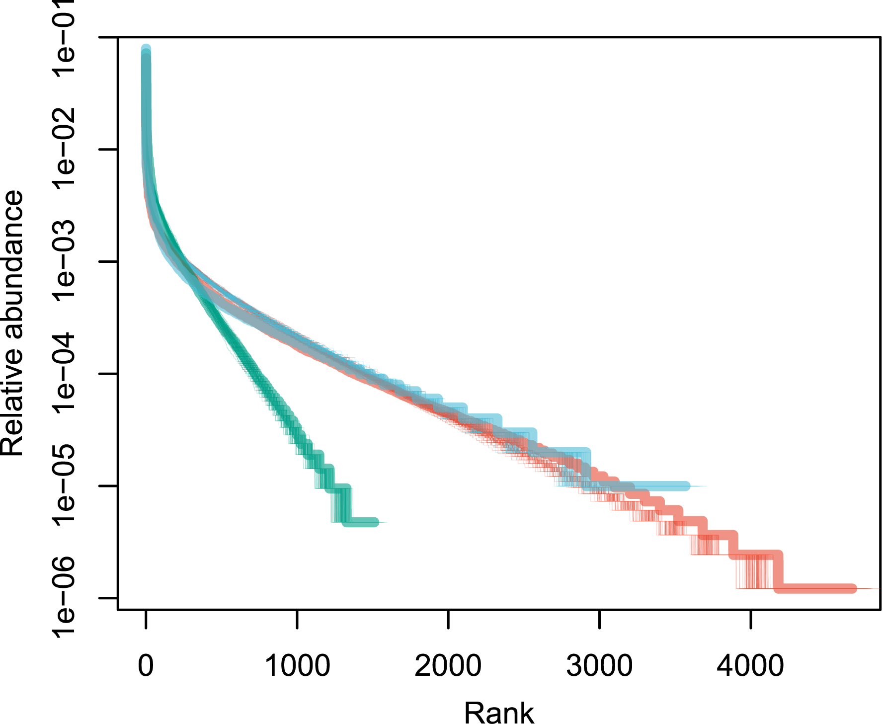
Patterns of species abundance and rarity are an important dimension of biological diversity. A species can be rare because it is limited by its physiology, by local biotic constraints on its abundance, or by its limited geographical distribution [1, 2, 3]. These diverse causes for rarity also reflect the fundamentally different reasons why species are threatened. Species that are locally abundant but geographically limited may be threatened with extinction if their habitat is transformed, as is the case with certain species of forest tree in the tropics. Highly specialized sap-sucking insects may be threatened because the trees on which they feed are removed. Finally, the degradation of restricted habitats can lead to the disappearance of species, as for example on the island of Saint Helens [4]. Although rare species exert great fascination, the question of why some species are abundant locally or regionally is no less interesting. The most abundant species are most relevant to many ecosystem processes. In a study of Amazonian rain forest trees, ter Steege et al. have shown that no more than 227 tree species make up half of the trees in this biome, out of more than 6700 species [5]. These were called hyperdominant species. Patterns of abundance for Amazonian rain forest trees [5] are represented in Figure 1 for illustration.
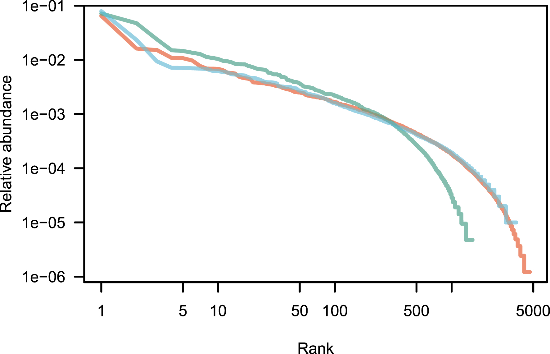
Rank abundance distribution of tropical tree species in three continents. These empirical distributions are scaled such that the sum of the relative abundances is equal to one. Red: Amazon; green: tropical Africa; blue: Southeast Asia. Data from [6].
The motivation for this contribution is to understand the processes underlying regional patterns of species abundance. One way to contribute to this research is to ask to what extent empirical species abundance distributions deviate from those of regional species pools generated purely from random processes. Here, I provide a self-contained treatment of neutral models of relevance in the study of species abundance distributions, together with a code for the algorithms in the R statistical language. Then I illustrate this method with regional species abundance data for three tree flora (Amazonia, Africa, Southeast Asia).
The neutral theory of biodiversity and biogeography [7] has emerged from the mathematics inspired by population genetics theory of the 1970s, and it has generated much debate in ecology. The theory has shed light on questions such as: how are the sampled individuals distributed between species? how many species remain to be discovered after a given number of individuals have been sampled? How representative are samples of larger ecological communities? When I was invited to contribute to the pages of this journal, I took opportunity to return to a debate on neutral models of species abundance that have animated the scientific community in ecology. Neutral models are now in the toolkit of ecologists for the analysis of species abundance [5]. Yet, many important results on neutral models tend to be overlooked in the modern literature and regularly rediscovered [8]. In addition, since the 1970s, important research in probability theory has been developed [9, 10, 11, 12, 13, 14], some of which is relevant to quantitative research on biodiversity.
This study explores models of species abundance that mimic the process of species discovery in a real situation, where individual organisms are identified to the species one at a time. The first organism is always a new species in the sample, the second may be a representative of the first species or of a new species, and so on. For such a model to make sense, it is assumed that organisms are identified one by one, through a classical taxonomic study. Bulk identification methods, using mass sequencing of environmental DNA for microbial species provide a different context to the study of biological diversity in that species are substituted for molecular operational taxonomic units, and individuals are not always observable or even clearly defined [15]. With that limitation in mind, it is still helpful to explore the patterns of species abundance in discrete assemblages of organisms [16]. The goal here is to return to known mathematical formulation of neutrality, provide several representations of the model and show that these representations are quite flexible.
Here, I first review the mathematical foundations of two standard models of species abundance, the canonical neutral model, and a spatially subdivided version of this model. I also discuss a model that has not been explored in the context of species abundance distributions, which models the hypothesis that the addition of species to a community may increase the resources and biotic interactions, making that community hospitable to a greater number of species, or in short “diversity begets diversity”, as proposed by Whittaker [17]1 . It is curious that this “diversity begets diversity” model has never received proper quantitative mathematical treatment in the ecological literature and one aim of this contribution is to promote this discussion [9, 11].
In Section 2, I present the fascinating mathematical results associated with three neutral models. In Section 3, I illustrate the application of these models to practical examples of parameter inference for empirical samples of tropical forest trees. Finally, I discuss the possible ramifications of the theory of random partitions for the study of empirical patterns of biodiversity.
2. Three neutral models of biodiversity
In ecology, models have been referred to as neutral in the sense that individuals all have the same prospects of reproduction and mortality, whatever the species to which they belong [20]. In probability theory, the more general notion of exchangeability is defined: a model is exchangeable if the probability distribution of the class abundances {n1, n2, …, nk}, where ni is the abundance of species i, does not depend on the labels of the classes [21, 22]. This property is essential in order to obtain exact mathematical results on the probability distribution of the model. This probability distribution, when known, can then be used as a likelihood function to compare the model to empirical species abundance distributions. In Section 2.1, an intuitive construction is provided in the form of urn models.
Model 1 is the canonical neutral model, for which the probability distribution of species abundances is the Ewens sampling formula [23], explained in Section 2.2. I also present the species individual curve for Model 1, and the Griffiths–Engen–McCloskey formula, which allows samples conforming to Model 1 to be drawn in a time proportional to the number of species k rather than the number of individuals n. Models 2 and 3 are two possible generalizations of Model 1. Model 2, presented in Section 2.3, assumes a spatially subdivided system, with limited dispersal between local sites. Under general assumptions, this Model 2 is also associated with a probability distribution for species abundances, and the model parameters can be estimated by maximal likelihood estimation. The second generalization, Model 3 (Section 2.4), implements the “diversity begets diversity” model. It turns out to be a equivalent to a model first developed in [9], with the same properties as the canonical neutral model but with the addition of one parameter.
2.1. Urn model representation
The process of species discovery can be summarized in generic terms using so-called urn models [24]. The “urn” represents the system (here, a sample, or an ecological community), and it is populated by “balls”, which represent objects (here, individuals). The objects may belong to two or more classes, which are usually represented by the color of a ball. The urn representation is relevant when an operator picks balls and performs a number of operations based on this sampling. A lottery is an example of a game that can be represented as an urn model, other examples including election systems [25, 26] or sports [27].
In the Pólya urn model [28, 24], an urn is initially filled with ni balls of color i, and the balls are drawn one by one, being replaced in the urn after its color has been observed. The construction process is as follows. When a ball is drawn, it is replaced in the urn together with a new ball of the same color. The most abundant color tends to be selected more often, so its abundance increases more rapidly. This Pólya urn model resembles the species sampling process, where a color symbolizes a species. Note that even if the process is stochastic, the abundance of each species depends on the initial condition of the system, i.e., the initial abundance of the species.
A slight variant of the Pólya urn model, due to Hoppe [29], is directly related to the problem of species sampling. It assumes that initially the urn contains a single black ball. The construction process is as follows. When the black ball is picked, it is replaced in the urn together with a ball of a completely new color. When any other ball is picked, it is replaced in the urn together with another ball of the same color. All the colored balls have the same chance of being chosen, which we define as a unit “weight”. In contrast, the black ball has a weight 𝜃, which is a positive real number. The parameter 𝜃 is proportional to the probability of adding a new color in the urn per iteration. This method yields a partition of the colored balls, and this partition depends on the single parameter 𝜃. This is the basis of Model 1 presented below, also called the “canonical neutral model”. It is a drastic simplification of reality, but is amenable to exact probabilistic results.
In large biological assemblages of organisms, geographical structure can become an important factor, and can invalidate the assumption of perfect mixing, i.e., the assumption that there is a single urn from which one samples the balls. For example, the Amazon is a large collection of trees (on the order of 4 × 10¹¹, see [5]), covering more than 6 million square kilometers, and assemblages of tree species differ west and east of the Amazon. Spatially subdivided models have been developed to account for this effect, where local sites are considered as a dispersal-limited sample of the regional pool [7, 30, 31]. The goal is to predict the local distribution of individuals between species in a local community, as a function of immigration rates and regional species diversity [7, 32, 33]. The influence of space on the canonical neutral model is discussed in Model 2 below.
In Model 3, the diversity begets diversity model, the rate of species appearance depends on the number of species in the system, which is denoted kn (the subset n is because the number of species depends on n, the number of individuals). As will be explained below (Section 2.4), one definition of this model is through an urn scheme, sometimes referred to as the Blackwell–MacQueen model [34, 9, 11]. After n − 1 individuals have been sampled, the probability of sampling an altogether new species (i.e., the probability of sampling the black ball) is equal to (𝜃 + 𝜎kn)/(𝜃 + n), so for any value of 𝜎 > 0, the probability to pick a new species is proportional to the number of existing species kn. In the special case 𝜎 = 0, this model is equivalent to the Hoppe urn model (Model 1). The probability of adding one individual to species i (i.e., the probability of sampling a colored ball) is equal to (ni − 𝜎)/(𝜃 + n), so each of the colored balls is picked slightly less often than expected by chance, and the rarest colors, represented by a single ball in the urn, are counter-selected. Biologically, rare species are likely to be less viable than expected by chance due to reproductive difficulties, both pre- and postzygotic [35, 36, 37]. Crucially, the complete sampling theory is known for this third urn model, as described below, so it lends itself to statistical inference [9, 11].
2.2. Canonical neutral model (model 1)
The first model describes a natural partition of n objects into k classes. This partitioning could concern many real-life situations, and has been applied in population genetics (number of allelic copies in a population, [23]), linguistics (number of word occurrences in a book [38]), and ecology (species abundance in a sample [39]). The question of how to partition discrete collections is also relevant to many other fascinating problems in mathematics [13, 14]. All the results in this section are classic but they are still provided as they provide essential context to Models 2 and 3. An excellent introduction is found in Ewens’ textbook (2004 edition, Chapters 3, 9, and 11, [8]).
In a sample of organisms, let us assume that the species have been labeled: the species differ in detectable ways, such as a taxonomic feature. We denote ni the abundance of species i, and
In the Hoppe urn model, step one draws the black ball with probability one, generating one new species. At the nth draw, n − 1 individuals have been sampled, and the probability of sampling an altogether new class (or color) is equal to 𝜃/(𝜃 + n), while the probability of adding one object to class i is equal to ni/(𝜃 + n). The Hoppe urn model generates a population of n objects, and patterns of class abundance are parameterized only by 𝜃. This construction turns out to be equivalent with Fisher–Wright model of population genetics [29, 8], or the dispersal-unlimited neutral model in ecology [40]. Consider a time-dependent system of N individuals such that all individuals die exactly at the end of the time step and are replaced by a multinomial draw of their offspring. In addition, with probability 𝜈 they are replaced by a totally new species. This means that new species can arise at a rate N𝜈 = 𝜃 (new species per time step). This system is assumed to be large in the sense that any sample n verifies n ≪ N. This process soon reaches a dynamic equilibrium where the appearance of new species is balanced by the extinction of rare species. Hoppe [29] has shown that the urn model generates a typical configuration of the above model at dynamic equilibrium.
In the Fisher–Wright model, the probability F2(t) that two randomly chosen individuals belong to the same species at time t is computed as follows [41, 8, 42]. For two individuals to belong to the same species, none of the two individuals can be a new species (probability (1 − 𝜈)2), and they can descend from the same parent (probability 1/N) or from two different parents already of the same species at the previous time step (probability F2(t − 1)). This reasoning is summarized in the equation: F2(t) = (1 − 𝜈)2(1/N + (1 − 1/N)F2(t − 1)). At dynamic equilibrium, F2 = F2(t) = F2(t − 1), and substituting in the equation, one finds F2 = 1/(1 − N + N(1 − 𝜈)−2). For N large and 𝜈 small, this results in: F2 = 1/(1 + 𝜃). This result is equivalent with the Hoppe urn model, since the probability of picking any one ball in the urn is 1/(1 + 𝜃). The same reasoning can be applied one step further to the probability of picking three individuals of the same species F3(t). Three situations can arise: (i) all three could descend from the same parent (probability 1/N2), (ii) they could descend from two parents (probability 3(N − 1)) already of the same species at time t − 1 (probability F2(t − 1)), or (iii) they could descend from three different parents (probability (N − 1)(N − 2)) already of the same species at time t − 1 (probability F3(t − 1)). At dynamic equilibrium, the formula reads: F3 ∼ 2/(2 + 𝜃)F2. This reasoning for two and three individuals can be extended to compute the probability of picking n individuals of the same species [23], which is Fn = (n − 1)!/(𝜃(𝜃 + 1)⋯(𝜃 + n − 1)).
The denominator of this expression, 𝜃(𝜃 + 1)⋯(𝜃 + n − 1), is an important mathematical quantity in this theory, and for this reason it deserves a specific notation: 𝜃(n) = 𝜃(𝜃 + 1)⋯(𝜃 + n − 1), which is called the increasing factorial power, or sometimes the “Pochhammer symbol”. 𝜃(n) may be expressed in terms of the usual Gamma function as follows: 𝜃(n) = 𝛤 (𝜃 + n)/𝛤(𝜃). An expansion of 𝜃(n) as a polynomial is known and it turns out to be useful below:
| (1) |
The above calculus on the probabilities Fn suggests that the computation of the complete probability distribution of the state {n1, n2, …, nk}, denoted p𝜃(n1, n2, …, nk), is possible. Ewens [23] has computed p𝜃(n1, n2, …, nk) as a closed-form expression, and Karlin and McGregor have provided a formal proof for this formula by recurrence [43]. This result is known as the Ewens sampling formula [13, 14]:
| (2) |
| (3) |
A first natural question is how many classes, or species, are in a sample of n individuals given the parameter 𝜃. From the Ewens sampling formula, the probability P𝜃, n(k) of finding k species in the sample of size n must be proportional to 𝜃k/𝜃(n), and since P𝜃, n(k) is a probability distribution, then
| (4) |
| (5) |
| (6) |
It may also be shown that the variance of k is equal to
| (7) |
Now, defining the log-likelihood function for Model 1 as Lk(𝜃) = ln P𝜃(k) from Equation (4), the maximum likelihood estimate of 𝜃,
| (8) |
In the literature on species diversity estimation, the estimated number of species in a sample
| (9) |
Finally, the following result turns out to be useful. A second generative process, the residual allocation model, has been shown to converge to the Ewens sampling formula. This construction has been popularized under the name Griffiths–Engen–McCloskey model by Ewens [8], in light of the pioneering works of [39, 48]. Let {W1, W2, …, Wk} be a vector of independently identically distributed random numbers drawn from the beta probability distribution with parameters (1, 𝜃): Beta(1, 𝜃) = 𝜃 (1 − W)𝜃−1. Let us define the variables {V1, V2, …, Vk} as follows:
| (10) |
2.3. Neutral model with dispersal limitation (model 2)
Spatial extensions of Model 1 have been developed early on in the context of population genetics [41, 30, 51], with subsequent applications in ecology and biogeography [52, 7]. One possible framework is as follows: a region is considered as a collection of K local sites (“demes” in the parlance of population genetics), and each local site has a total size {N1, …, NK}. Within a local site, individuals interact directly, whereas local sites are only connected through migration. This framework is the multi-deme model of population genetics [53, 30] and the metapopulation model of population dynamics [52]. Within-site processes (local reproduction, interactions) are the dominant processes over small time scales compared with the genealogical processes occurring across local sites and over much longer time scale [30]. A similar setting arises in spatial interacting particle systems, such as chemical reactions [54, 10].
An historically important special case, due to Hubbell [7], is one where a single site is sampled. Conceptually, this model is parameterized by the same parameter 𝜃 as above, which describes the regional species pool. An additional parameter m (0 ⩽ m ⩽ 1) represents the probability that a new individual appears in the focal community through immigration rather than due to local reproduction. If m ∼ 1, all the local recruits are immigrants, and the local structure becomes irrelevant, in which case the Ewens sampling formula Equation (2) applies, together with the results of the previous section. In the more general case of an arbitrary parameter m, a closed-form solution of the general sampling formula does exist and it generalizes Equation (2) [40, 32]. With I = m/(1 − m)(n − 1) a rescaled migration parameter, the generalized version of the sampling formula is (see Equation (6) in [32]):
| (11) |
| (12) |
Let us now turn to Model 2. One far more interesting model of spatially subdivided populations is the K-deme model, with K local samples (or demes), of size {N1, …, NK}. Assume that the regional relative species abundance distribution is given by {x1, …, xk}, where xi is the regional relative abundance of species i, and ∑i xi = 1. Denote {n1j, …, nk j} the species abundances in deme j, such that ∑i nij = Nj. Finally, assume that each local deme j has an immigration rate mj, with mj ∈ [0,1] (or equivalently the rescaled immigration rate Ij = mj/(1 − mj)(Nj − 1)). This model could describe an archipelago with K islands, some far away from the continent (m ≪ 1) and others closer, as in the insular theory of biogeography [56]. In this case, the sampling formula px,I(nij), i ∈ {1, …, k}, j ∈ {1, …, K} can be written as [33]:
| (13) |
| (14) |
with C a constant, and using again the equality x(n) = 𝛤 (x + n)/𝛤(x).
Note also that px,I(ni, j) is the product of the probabilities for each of the K demes. The maximum likelihood estimate of Ij is obtained for the condition: ∀j, ∂ Lx, n i, j(I)/∂ Ij = 0, and this implies that the migration parameter Ij can be estimated independently of all other model parameters through the following equation, for all j:
| (15) |
2.4. Neutral “diversity begets diversity” model (model 3)
A second natural extension of Model 1 is one where the probability of creating new species increases with the number of species in the sample. The idea of this model is that species entering a community generate the conditions for the establishment of more species than originally possible. Formally, the rate of species appearance is not strictly equal to 𝜃 but increases with the number of extant species k as 𝜃 + 𝜎 k, where 𝜎 is a new parameter in the model compared with Model 1.
As outlined above, let us first represent this model as an urn scheme. After n − 1 individuals have been sampled, the probability of adding one individual to species i (i.e., sampling a colored ball) is equal to (ni − 𝜎)/(𝜃 + n), while the probability of sampling an altogether new species (i.e., sampling the black ball) is equal to (𝜃 + 𝜎k)/(𝜃 + n). In the special case 𝜎 = 0, this model is equivalent to the Hoppe urn model (Model 1). Values 1⩾𝜎⩾0 imply that rare species tend to be picked less, and that more new species arise. As 𝜎 → 1, the probability of picking a singleton species vanishes, and at 𝜎 = 1, species cannot increase in abundance and each new individual represents a different species. This model was introduced by Blackwell and MacQueen [34] in the early 1970s, then was formally studied by Pitman and colleagues [9, 58, 59].
In Model 3, the expected number of species k is given by the summed probability of picking the black ball at each step:
| (16) |
| (17) |
| (18) |
Let us now turn to the existence of a sampling formula for Model 3. Pitman has shown that a sampling formula analogous to that of Ewens can also be derived in this case [58] and that it has the following form:
| (19) |
| (20) |
| (21) |
In empirical species abundance studies, one objective is to infer the values of model parameters 𝜃, 𝜎 given the observed vector n1, n2, …, nk. In the case of the Ewens sampling formula, the number of species k and the sampling size n are jointly sufficient to estimate the parameter 𝜃. It is no longer the case in this two-parameter Model 3. However, it remains true that Equation (21) can be used to define a log-likelihood function Ln(𝜃, 𝜎) = ln p𝜃,𝜎(n1, n2, …, nk), which takes the form:
| (22) |
| (23) |
Finding best-fit parameters 𝜃, 𝜎 can be obtained by solving these two equations jointly, but it is simpler to maximize the function Ln(𝜃, 𝜎) (Equation (22)). The numerical problem of finding 𝜃, 𝜎 given the vector n is therefore easily resolved (see next section for a numerical implementation).
Importantly, species abundance distributions for Model 3 can be generated through a random allocation model (Griffiths–Engen–McCloskey construction) similar to that in Model 1. Let {W1, W2, …, Wk} be a vector of i.i.d. random draws with Wi from the probability distribution Beta(1 − 𝜎,𝜃 + k𝜎), with 0 ⩽ 𝜎 ⩽ 1. Define the variables {V1, V2, …, Vk} as follows:
| (24) |
2.5. Numerical analyses
To perform empirical analyses, I have written the package neutr in the R Statistical Language [61], available at https://github.com/jeromechave/neutr.
Parameters can be fit against the empirically observed species abundance data. For Model 1, function optim.ewens() optimizes Equation (2). It has the empirical species abundance as an argument and returns parameter 𝜃 and the maximal log-likelihood value. For Model 2, the function optim.multideme() takes as argument a matrix with entry the abundance nij (species i in deme j) and it optimizes Equation (13). This function returns a vector of parameters Ij = mj/(1 − mj)(nj − 1), one per deme, and mj. Importantly, the optim.multideme() function assumes that the regional species abundance distribution is the sum of all local species abundances. For Model 3, the function optim.pitman() takes the empirical species abundance as an argument, plus initial values of 𝜃, 𝜎 and returns the best-fit parameters 𝜃, 𝜎 and the maximal log-likelihood value based on Equation (22).
Another set of functions return typical species abundance distribution generated by Models 1 and 3. Package neutr includes the function generate.hoppe.urn0() that generates a species abundance distribution according to the Hoppe urn model (Model 1). It takes parameter value 𝜃 and sampling size n as an argument, and returns one possible species abundance distribution and the species number
The three models can also be compared: Model 1 is nested within both Models 2 and 3, but the number of kp parameters vary (kp = 1 for Model 1, kp = K for Model 2, and kp = 2 for Model 3). It is possible to compare the models based on some form of the Akaike Information Criterion [62].
Package neutr bears resemblance with package untb [63], which implements Model 1, but not its Griffiths–Engen–McCloskey construction. Also, packages ecolottery [64] and package GUILDS [55] both implement Models 1 and some forms of Model 2 based on the coalescent, as first proposed by [40]. To my knowledge, Model 3 and its Griffiths–Engen–McCloskey construction have never been implemented in a R package.
3. Application to the tropical tree flora
3.1. Datasets
An empirical application of the above theory is now provided for three large empirical data sets taken from numerous tropical forest inventories around the world and reproduced as a Supplementary Information of [6]. It contains a total of over a million sampled trees all identified to the species, for a total area of forest sampled of 2324 ha (23.24 km2; summary in Table 1). This is a huge sampling size, although it is very small compared with the ca. 10.7 million km2 of tropical forests [65]. Since the exact species name is not reported in this data set, it is impossible to estimate the exact number of species in total, although the species overlap across continents is small, and the species total is likely to be close to the sum (9765 species). The raw data is plotted as a rank-abundance curve in Figure 1.
Statistics of the data used in this study
| Region | Nb trees | Nb species | Cumul. area (ha) | Nb plots |
|---|---|---|---|---|
| Amazon | 821,670 | 4670 | 1590 | 1417 |
| Tropical Africa | 210,313 | 1509 | 504 | 483 |
| Southeast Asia | 100,152 | 3586 | 201 | 230 |
| Total | 1,021,974 | NA | 2324 | 2130 |
The table reports the total number of trees sampled, total number of species, cumulative sampled area (in hectares, ha), and total number of permanent sampling plots in the biome. Data from Ref. [6].
Briefly, the data have been obtained using a standard method in tropical forest science: standard areas, usually squares of one hectare (100 × 100 m), are positioned on the ground, and all trees with at least 10 cm in trunk diameter are mapped, tagged using a permanent tag (in plastic or metal), and identified to the species [66]. Establishing a permanent forest inventory plot requires several days of work in the field, and complete botanical identification is usually much more time consuming. The above data set is therefore the result of a long term vision, and hard work of a large scientific community from across the tropics.
3.2. Results
For Model 1, the estimate of parameter 𝜃 for all three data sets is provided using the empirical values of n and k with Equation (6). I used the empirical values of 𝜃 and Equation (10) to produce 1000 neutral distributions for each of the three empirical distributions. Figure 1 reveals that the fit to the data is not bad, except for a small number of the most abundant species (see [67] for a similar pattern). It is therefore interesting to explore if the goodness of fit improves when the top species are removed.
To estimate the goodness of fit, one method is to define a distance between the observed Pobs and the theoretical Ptheor distributions. I use the Kullback–Leibler distance, defined by
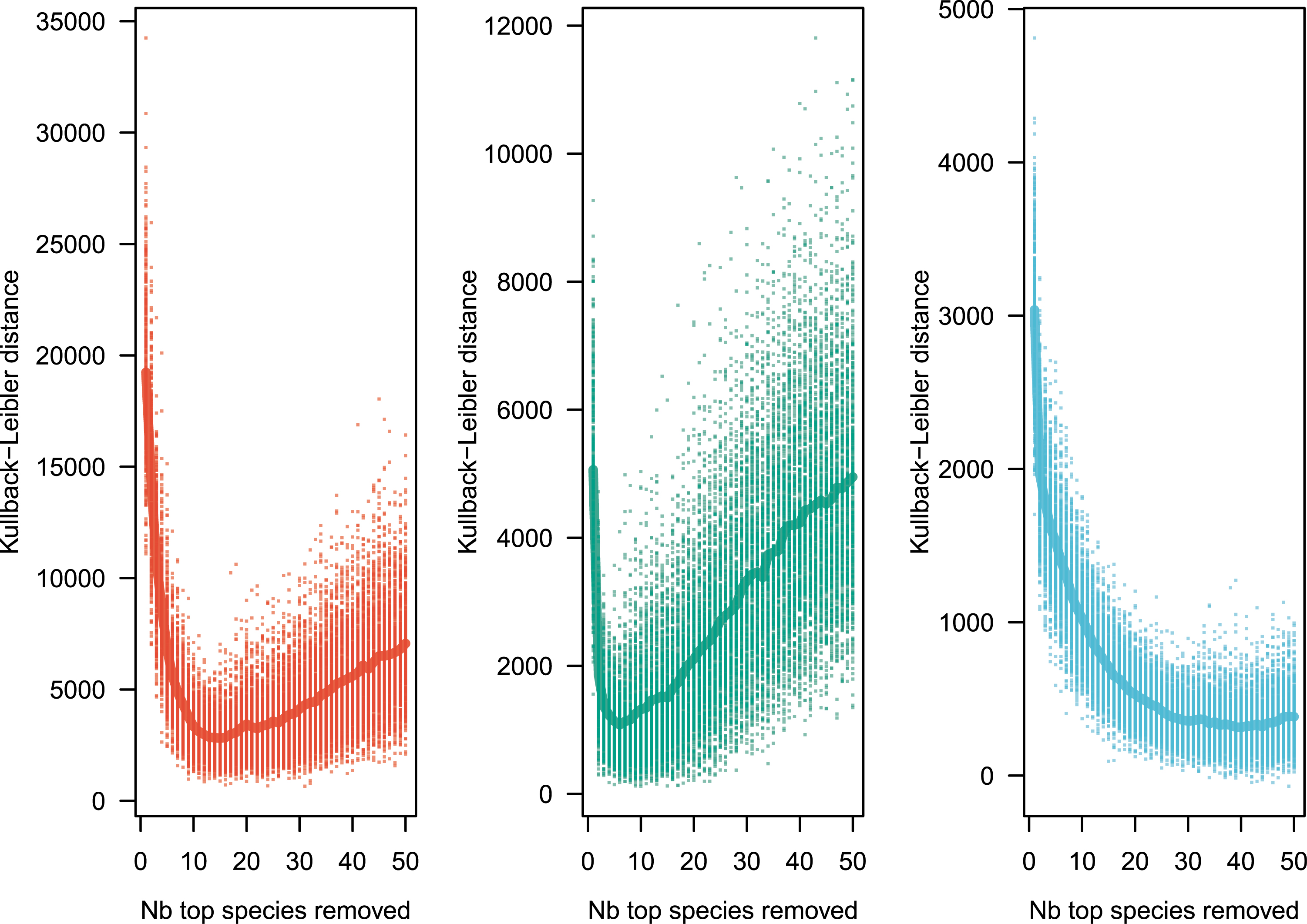
Kullback–Leibler distance between observed and simulated distributions replicated 1000 times, after sequentially removing 1 to 50 of the most abundant species. The minimal Kullback–Leibler distance, number of species to remove to minimize the distance, and 𝜃 are reported in Table 2. Color codes as in Figure 1.
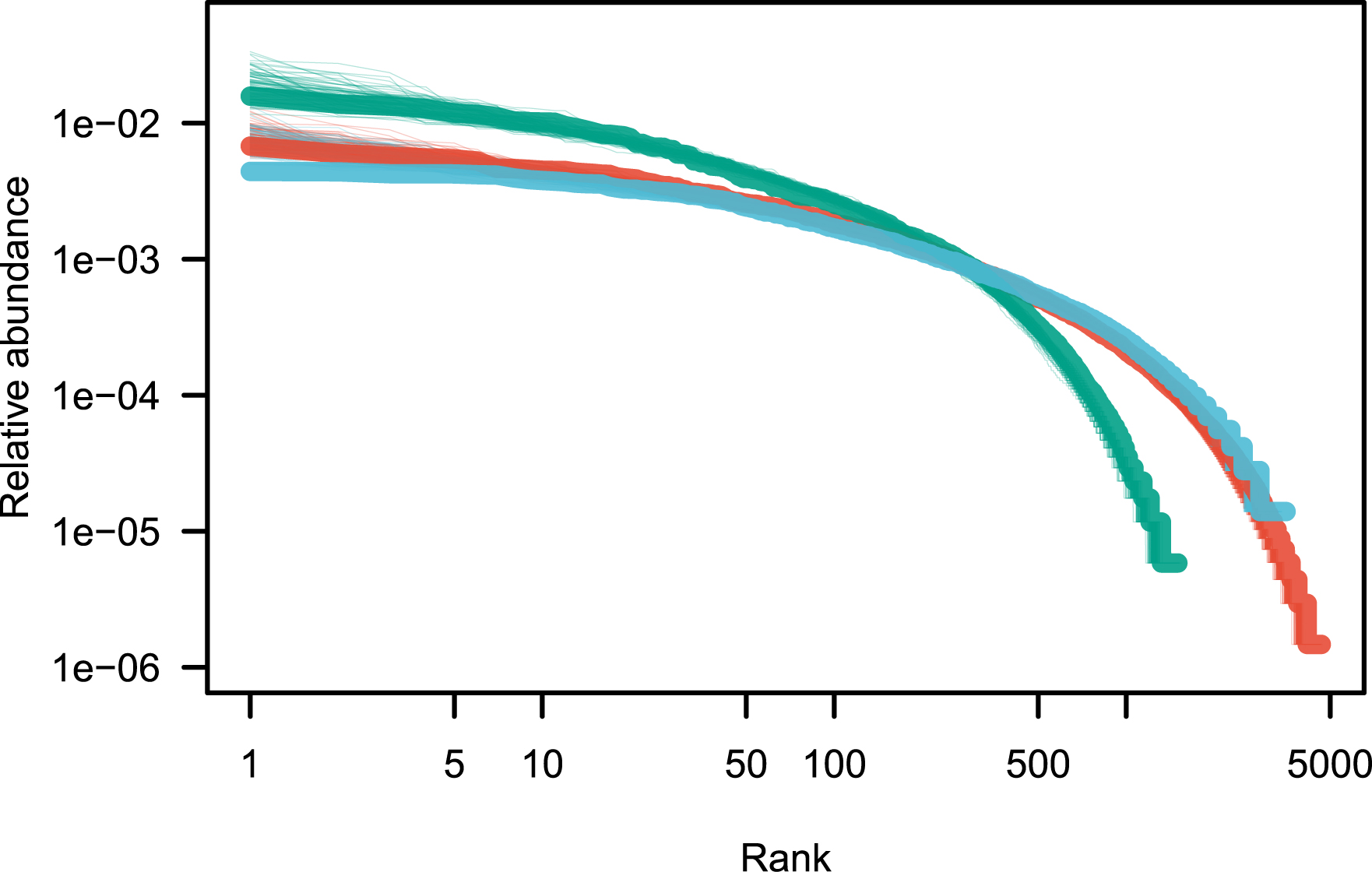
Fit of the rank abundance distributions after removing the ultradominant species (see Table 2). Color codes are as in Figure 1.
Best fit of the canonical neutral model after removing a number of the top species (see Figure 2 for an illustration)
| Region | Initial 𝜃 | Min. Kullback–Leibler | Nb. of ultradominant species | 𝜃 of best model |
|---|---|---|---|---|
| Amazon | 654.3 | 2748.6 | 13 | 673.19 |
| Tropical Africa | 219.7 | 1077.0 | 6 | 226.69 |
| Southeast Asia | 726.8 | 299.9 | 40 | 778.23 |
Empirical values of parameter 𝜃 are reported before (first column) and after (last column) the ultradominant species have been removed. Column “Min. Kullback–Leibler” reports the mean value of the minimal Kullback–Leibler distance between model and observations (average across 1000 values).
The multideme model (Model 2) can be fitted with the maximization of Equation (15). The distribution of m values, which represent the fraction of individuals drawn from the regional pool rather than from the local site, peaks at m = 0.122 for Amazonia, m = 0.094 for Africa and m = 0.127 for Southeast Asia (Figure 4). This shows that local sites are dispersal-limited in similar ways across continents on average. Sites-specific parameters m could be interpreted as an environmental filtering effect, since m measures how dissimilar the local assemblage is from the regional one [33].
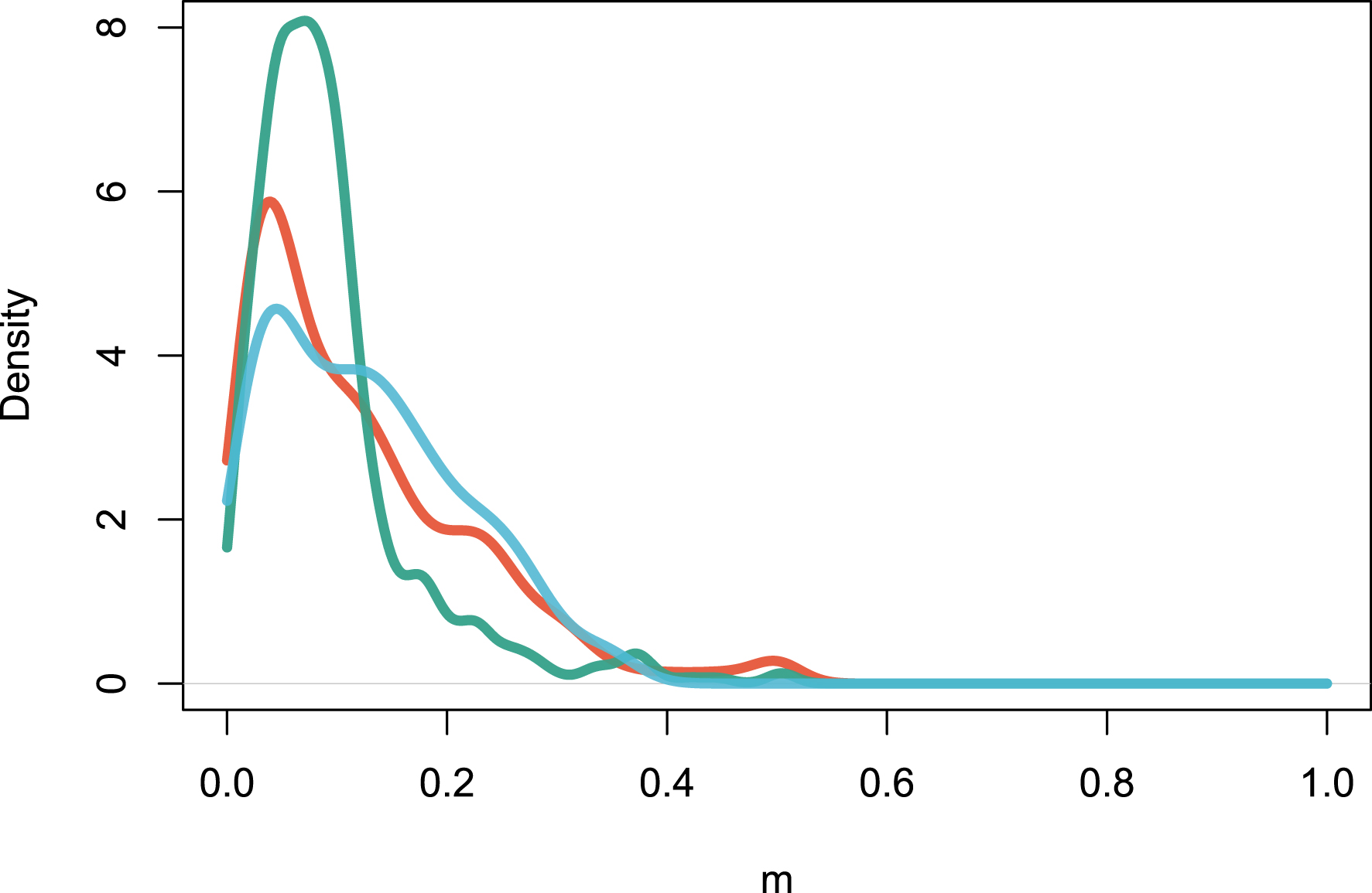
Estimation of the local m parameters for all the sites in the three continents. The figure reports the density distribution of m values. Color codes are as in Figure 1.
A fit of the data set against the two-parameter Model 3 is illustrated in Figure 5. The fit is not improved for the Amazonia and tropical Africa data (𝜎 values <10−7), and barely so for Southeast Asia (𝜎 = 0.034). Thus, for these data sets, Model 3 does not result in a better fit of the data than Model 1.
Fit of the rank abundance distributions (thick solid lines) against Model 3 (n = 100 simulations, thin solid lines), in linear–log axes, which allow a better display of the tail of the distribution (rare species). Compare with Figure 1 for a similar representation in log–log axes. Color codes are as in Figure 1.
The neutral model represents well tropical tree species abundances at regional scale, and this finding is used to extrapolate species numbers [5]. Assuming that the Amazonian tropical forest covers about 6.3 million km2, with an average 500 trees per hectare, the estimated number of trees is N ≈ 3.15 × 10¹¹. Using the value of 𝜃 reported in Table 2 and N in Equation (6) yields
Estimated number of species in tropical forests based on an extrapolation of Model 1
| Region | Area (M km2) | Nb trees (estimated) | Nb species | Nb species with at least 50 ind. |
|---|---|---|---|---|
| Amazon | 6.3 | 3.15 × 10¹¹ | 13,081 | 10,141 ± 91 |
| Tropical Africa | 2.9 | 1.45 × 10¹¹ | 4,462 | 3,477 ± 51 |
| Southeast Asia | 1.1 | 0.55 × 10¹¹ | 13,186 | 9,915 ± 90 |
The estimated number of species is provided together with the estimated number of species with at least 50 individuals.
4. Discussion
4.1. Three neutral models
The three models presented here are only a few examples of the many systems that can be framed as urn models [24]. The reader may be surprised to read no mention of the coalescent theory, even if Model 1 is the key building block of this theory [70, 12]. The coalescent is a powerful approach, but the choice was made here to focus solely on species abundance distribution and efficient numerical analyses can be performed without resorting to coalescent models. There is no doubt that exploring further applications of the coalescent in ecology should be a rewarding effort.
The three models presented here are neutral in the following sense. All three describe a partition of the collection into disjoint subsets (classes), such that the objects within each class are interchangeable, and the abundance ni⩾1 within class i is a random number that fully describes the class. The models are thus fully described by the probability distribution p(n1, …, nk) of the sequence of random numbers {n1, …, nk}, where
Another property common to exchangeable models is that a random partition following Equations (10) and (24) define a size-biased partition of {V1, V2, …, Vk} that can be used to define an ordered series of relative abundances Pi, i ∈ {1, …, k}, with P1⩾P2⩾⋯⩾Pk, such that
The one-parameter (𝜃) Model 1 is a special case of a more general two-parameter (𝜃, 𝜎) Model 3. When 𝜎 = 0, Models 1 and 3 are equal. Model 3 turns out to have a biological interpretation as a species abundance model where diversity begets diversity: new species tend to be picked with probability (𝜃 + k𝜎)/(𝜃 + n) (0 ⩽ 𝜎 ⩽ 1), when k species are already present, so more often than expected by chance. With respect to the asymptotic scaling regime n ≫ 1, Equations (9) and (18) are two well-known scaling relationships in ecology and there has been much literature on whether the species accumulation curve
The dispersal-limited neutral model of [7] is historically important in the context of ecology and biogeography. However, Hubbell’s two-parameter (𝜃, m) generalization of Model 1 is not framed as an urn model or a random allocation model. An urn representation of Hubbell’s model is possible, but it is not straightforward2 . This is a special form of a hierarchical urn construction, such that the construction of the second urn depends on that of the first urn, but not the other way around. Here, I define Model 2 as a neutral model of K subdivided assemblages, or multi-deme model, a more useful alternative in practical situations. Though only one result is presented and studied here, many other results have been obtained, and it is an area where coalescent based numerical analyses are most useful [51, 12].
4.2. Implications for tropical forests
A remarkable feature is that neutral models fit extremely well tree species abundance data [7, 5]. The only departure from this neutral fit appears to be for the most abundant species, which I have here informally called ultradominant species. Ultra-dominant species are the most abundant species that tend to depart from the prediction of the canonical neutral model (Model 1), and a simple empirical method is proposed here to detect these species. When ultra-dominant species are removed from the analysis, the neutral model reproduces empirical observations extremely well in the three regional tropical tree data sets explored here (Figure 2). The nature of ultra-dominant species is unclear, but it would be interesting to explore the commonalities of ultra-dominant species, and possible biological explanations for their occurrence.
A second insight from this analysis stems from the fit of the multi-deme model (Model 2) to the same three regional tropical tree data sets. The finding of Figure 3 is that most local sites significantly depart from a hypothesized random sample of the regional species pool, detected by m values much lower than unity. In a dispersal-limited interpretation [7], this suggests that a relatively constant proportion of the reproduction events are local, the rest being immigration events. The alternative explanation is that biotic or abiotic effects exert a major influence on the floristic composition of each local community, and m < 1 values in the multi-deme model reflect these environmental filtering effects [33].
In the Ewens canonical model, 𝜃 is a natural measure of local diversity, which is a convenient property of the model. However, non-parameteric methods of biodiversity estimation have also been developed, and they are often presented as more robust than parametric methods [72, 73]. It is not the goal of the present contribution to discuss this issue at length. One known limitation of Model 1 is that the 𝜃 parameter cannot be estimated with confidence for small sample sizes. A method such as Model 2 may provide a useful alternative to Model 1 and it would be interesting to explore the scale dependence of the m parameter (i.e., how m varies with decreasing sample sizes n).
The notion of neutrality has generated a heated debate in ecology [7, 20, 74, 75, 76]. Part of the debate has been motivated by a narrow definition of neutrality. The questions raised relate to the fact that this model ignores so many important features as to become useless or event dangerous [77]. Species differ not only in abundance but also in ecological traits, and individuals within species also differ in size, metabolic capacity, and fitness. A second class of critiques of ecological neutrality is that tests of the theory are not robust because independent estimates of the parameters cannot be accessed [74]. A last class of critiques relate to the consistency of the ecological neutral model with respect to the dominant theory in ecology, niche theory, which interprets patterns of species occurrence in the light of competition between species [78]. Sampling methods that make the assumption of neutrality (in the sense of exchangeability), are however more general than commonly discussed in the ecology literature. One strength of these models presented here is that they are naturally associated with a method of exact inference, which makes it possible to compare model and data quantitatively. By analogy, the analysis of selectively neutral alleles in natural populations is a useful tool set of population genetics, and helps infer past population sizes, and phases of demographic expansions and bottlenecks [8, 79].
In ecology, the development of the neutral mathematical tool set has not been as rapid as in genetics. One limitation has been that, unlike in genetics, methods for analyzing huge data sets has been relatively less in need in ecology. The situation is changing now with the rapid rise of DNA-based ecology [15], in which samples are not of individuals but of sequences, and with applications in tropical forest research [80]. Provided that sequence abundance data can be interpreted biologically, the question of the structure of sequence abundance distributions can be explored with the same approach as outlined here.
Why should a model as simple as Model 1 provide such an excellent fit to regional tropical tree abundance data? The neutral hypothesis cannot be valid over ecological and evolutionary time scales. Yet, regional species assemblages result from such a myriad of local processes, both biotic and abiotic, that large enough samples of regional patterns average over these effects. Half a century ago, Robert H. Whittaker wrote [17]: “The enigma of the diversity of the tropical rainforest should be expected to open itself to no single key, and may be enigmatic to the extent we have yet to comprehend the full implications of biotic differentiation and interaction, the complexity […] that is feasible and has evolved in these forests”. To this day, this analysis still holds, and the successes of the neutral theory to replicate broad patterns remains a mystery. Even if the details of species persistence and coexistence may be explained by fundamentally different processes [2], the laws of large numbers provide important insights into key questions on the regional species abundance patterns.
Declaration of interests
The author does not work for, advise, own shares in, or receive funds from any organization that could benefit from this article, and has declared no affiliations other than his research institution.
Funding
I gratefully acknowledge funding from “Investissement d’Avenir” grants managed by the Agence Nationale de la Recherche (CEBA, ref. ANR-10-LABX-25-01; TULIP, ref. ANR-10-LABX-0041; ANAEE-France: ANR-11-INBS-0001), CNES long-term funding, the European Space Agency CCI-BIOMASS and FRM4BIOMASS projects. This research is product of the SynTreeSys group funded by the synthesis center CESAB of the French Foundation for Research on Biodiversity (FRB).
1 The hypothesis that diversity begets diversity has been extremely popular in the recent literature, yet the history of this catchy term is quite obscure. It is generally traced back to Robert H. Whittaker (1972, p. 216) [17] who writes that “facilitation of increase in species number in interacting trophic levels is reciprocal. We should thus expect diversity to increase in parallel on any adjacent trophic levels and, in fact, throughout the various groups of interacting species that the community comprises.” In fact similar ideas are already present in Allee et al. (1949) textbook on animal ecology [18, p. 695]. Vane-Wright (1978) referred explicitly to the diversity begets diversity mechanism in an evolutionary context [19].
2
Define two urns, the first with a black ball with weight 𝜃, the second empty. First, draw J balls from the first urn exactly as in the Hoppe urn scheme, generating the sequence of ball colors: