

1 Introduction
In NMR of high abundance nuclei such as 1H, precise quantification of magnetization intensities for the different types of nuclei is made difficult by the usual presence of homonuclear scalar couplings. For nuclei X in low abundance, such as 13C and 15N, heteronuclear broadband 1H decoupling during the acquisition enables simplification of the spectrum. But then, nuclear Overhauser enhancement may appear, which is incompatible with quantification. To remove it, a very long delay without any decoupling during 9 to 10 T1max of X nuclei will be necessary before next read pulse [1,2]. This makes the sequence, usually called inverse-gated-decoupling sequence, globally poorly sensitive [1]. Also, the decoupling RF field applied during the acquisition may disturb the system and induce instabilities. The peaks are then no longer Lorentzian and their quantification by means of Lorentzian simulations does not give adequate results. For all these reasons, it seemed us interesting to obtain quantitative decoupled spectra without applying any decoupling RF field.
Aue et al. first presented a method for obtaining a proton decoupled NMR spectrum without applying any RF field [3]. This was based on the diagonal projection of a 2D J-resolved absolute value spectrum and hence gave a spectrum with a poor spectral resolution. Bax et al. adapted this method for obtaining a better resolution and developed the ‘constant-time’ experiment [4], where the signal was detected a constant time after the 90° pulse instead after the spin echo. Unfortunately, the areas of the peaks were then no longer proportional to the equilibrium magnetization.
Woodley and Freeman [5] proposed a pattern-recognition algorithm that converts a two-dimensional NMR J-spectrum in a decoupled spectrum and efficiently eliminates all dispersion signals. Unfortunately, this technique fails in the presence of severe overlap and when signals have amplitudes at noise level. Nuzillard [6] showed that transforming the data of a J-resolved spectrum by means of linear prediction for the negative t1 values and then doing their F2 projection could give a similar result. Mutzenhardt et al. [7] developed a close procedure for obtaining pure absorption 2D J-spectra, by means of linear prediction for the negative t2 values. This method was supposed to give quantitative fully J-decoupled NMR spectra, but seemed rather complicate to implement in routine procedures.
Another approach was considered by Mahi et al. [8], who developed a mathematical treatment of NMR signal from a 2D J-resolved spectrum, called analytical decoupling.
Mahi et al. showed that this method could be applied either in 1H NMR or for other nuclei. They also suggested that this method appears suitable for quantitative studies. To our knowledge, the efficiency of this method for obtaining quantitative results has nether been estimated until now. The aim of this work is to evaluate it. First, the principle of analytical decoupling is described rapidly. Then, simulations of different NMR signals are performed. Finally, these signals are transformed by the analytical decoupling method and their intensities are studied.
2 Principle of the analytical decoupling
The whole method is described in [8]. We give here the main calculations. The signal of coupled magnetization detected after the spin-echo pulse sequence: D1 – 90° − τe/2 – 180° − τe/2 – Acq(t) is treated so as to obtain a spectrum without any indirect J coupling, as if it would be totally decoupled. For that, the delay τe is incremented regularly from 0 to the maximal value T. A signal M(t,τ) is then recorded, where τ is defined by the relationship: τ = T − τe. This signal M(t,τ) is then multiplied by exp[2 i π ν (t − τ + k T)], where k is a constant between 0 and 1 chosen by the operator, and doubly integrated in frequency and for the delay τ between 0 and T.
The corresponding integral can be approximated by the function:
| (1) |
In the case of a weakly coupled system of two spin 1/2 nuclei, the part of the signal M(t, τ) detected at frequency ν0 + J/2 transformed as described in (1) becomes:
| (2) |
Mahi et al. proposed to treat again S(t, k) so as to obtain a new time function whose intensity would be independent of the coupling constant [8]. For that, S(t, k) is multiplied by exp[2 i π ν′(t − τ + k T)] {1 + [α (kmax/2 – k)]2}–1 exp(−a k T), where the constants a and α are chosen by the operator, and doubly integrated in frequency and for k between 0 and kmax. This integral can be approximated to the value:
| (3) |
For a = T2*, the transformation by this way of the function S(t, k) written in Eq. (2) gives:
| (4) |
The signal is no longer modulated in phase but its amplitude still depends on its T2 by the term: which may also induce an important attenuation.
Before being able to use optimally this method for quantification, one may wonder a few questions. In which way can one limit the attenuation and the distortions due to the treatment? What are the consequences of the approximate integrations made? Which values of the different parameters should one choose?
So as to answer these questions, we have made simulations of NMR signals and of Gaussian noise detected after a spin-echo sequence with the program Mathematica. The corresponding signals M(t,τ), obtained for a series of values of τ between 0 and T, were then treated by means of Eq. (1). When a signal resonating at a single frequency was detected, it was analysed in the time domain. S(t,k) and S(t) are complex functions of time. Their modules for t = 0 give the area of the corresponding peak in the phased spectrum obtained after Fourier Transform. They were studied for estimating the validity of quantification. The signals S(t,k) and S(t) could eventually be Fourier transformed and analysed in magnitude with the program Origin (Microcal) for observing the quality of the analytical decoupling.
3 Results
Magnetizations resonating at frequency ν0 + J/2 were simulated and treated by means of Eqs. (1) and (3) to obtain the demodulated signal S(t). Three values of J (1, 8, and 16 Hz) were considered. Other parameters of the simulated magnetizations were: M0 = 100, T2 = 0.5, T2* = 0.1, TAQ = 1.4 s, T = 1.44 s, 200 echo delays, F = 40. Other parameters introduced for the demodulation treatment where chosen as suggested by Mahi et al. [8]: a = T2* = 0.1, α = 44, kmax = 0.5, and the integration was performed for 100 values of k, regularly spaced between 0 and kmax. We performed these simulations for different values of the filter coefficient F′. The amplitude of S(t) at the origin was measured. The results are presented in Table 1 for the filter coefficient F′ between 100 and 160. One observes that for a given value of J, the amplitude of the signal depends a lot of F′. Similar fluctuations were still observed for larger values of F′, whereas the signal detected was even smaller.
Evolution of the magnitude ||S(0)|| obtained after the demodulation treatment as a function of F′ for three values of J
| J(Hz) | 1 | 8 | 16 | |
| F' = | 100 | 29.2 | 27.5 | 18.5 |
| 110 | 26.9 | 13.8 | 23.62 | |
| 120 | 87.8 | 102.4 | 110.5 | |
| 130 | 131.2 | 200 | 926 | |
| 140 | 958.25 | 471 | 240.7 | |
| 145 | 220.3 | 504.1 | 557.68 | |
| 150 | 202.3 | 197.393 | 387 | |
| 160 | 78.68 | 92.5 | 108.7 |
Unfortunately, the dependence of the signal as a function of F′ is not the same for the different J values. This transformation is then totally incompatible with quantification. Maybe the method could be more efficient with other values of a and α. But these preliminary results show that it should be used with circumspection.
In order to better understand the problems met in quantification and eventually get rid of them, we have studied the different steps of the transformation. First, magnetizations resonating at frequency ν0 + J/2 were simulated and treated by means of Eq. (1), for three values of J (1, 8, and 16), two values of F (100 and 40) and different values of k between 0 and 1. The other parameters were the same as previously. The magnitude of the signal S(t,k) at the origin, ||S(0,k)||, was measured for F = 100 (Table 2) and F = 40 (Table 3). Gaussian noise was simulated and transformed in the same way. It was drawn as a function of time and its maximal amplitude was measured. The aim of this comparison was to better understand the effect of the choice of F on the value of S(t,k). For the two values of F, the noise magnitude was independent of k: bmax = 11.4 when F = 40 and bmax = 20.2 when F = 100.
Evolution of the magnitude ||S(0,k)|| as a function of k and J for F = 100
| k | 0 | 0.01 | 0.1 | 0.3 | 0.5 | 0.7 | 0.8 | 0.9 | 0.95 |
| J = 1 | 33.1 | 37.8 | 45.3 | 82.1 | 147.9 | 260.7 | 347 | 436 | 552 |
| Δb (%) | 43.3 | 37.8 | 31. 6 | 17.4 | 9.67 | 5.48 | 4.12 | 3.28 | 2.59 |
| J = 8 | 33.9 | 39.2 | 45.22 | 84.4 | 145.5 | 259.8 | 348 | 433 | 533 |
| ΔJ (%) | 2.67 | 3.68 | –0.20 | 2.75 | –1.63 | –0.36 | 0.20 | –0.79 | –3.30 |
| Δb (%) | 42.2 | 36.5 | 31.6 | 16.9 | 9.83 | 5.50 | 4.11 | 3.30 | 2.68 |
| J = 16 | 32.9 | 38.18 | 47.5 | 82.0 | 149 | 260 | 350 | 452 | 528 |
| ΔJ (%) | –2.95 | –2.55 | 4.77 | –0.16 | 0.98 | –0.27 | 0.81 | 3.48 | –4.27 |
| Δb (%) | 43.5 | 37. 5 | 30.1 | 17.4 | 9.57 | 5.50 | 4.08 | 3.17 | 2.71 |
Evolution of the magnitude ||S(0,k)|| as a function of k and J for F = 40
| k | 0 | 0.01 | 0.1 | 0.3 | 0.5 | 0.7 | 0.8 | 0.9 | 0.95 |
| J = 1 | 24.16 | 29.31 | 24.16 | 82.6 | 148 | 268 | 357 | 603 | 551 |
| Δb (%) | 33.37 | 27.50 | 33.37 | 9.76 | 5.43 | 3.01 | 2.26 | 1.34 | 1.46 |
| J = 8 | 26.48 | 28.03 | 26.48 | 84.4 | 145 | 270 | 343 | 610 | 529 |
| ΔJ (%) | 9.60 | –4.37 | 9.60 | 2.14 | –1.95 | 0.56 | –3.78 | 1.09 | –4.00 |
| Δb (%) | 30.44 | 28.76 | 30.44 | 9.55 | 5.54 | 2.99 | 2.35 | 1.32 | 1.52 |
| J = 16 | 29.13 | 27.49 | 29.13 | 80.7 | 150.7 | 264 | 363 | 609 | 534 |
| ΔJ (%) | 20.57 | –6.21 | 20.57 | –2.28 | 1.59 | –1.41 | 1.82 | 1.00 | –3.17 |
| Δb (%) | 27.67 | 29.32 | 27.67 | 9.99 | 5.35 | 3.05 | 2.22 | 1.32 | 1.51 |
So as to estimate the pertinence of the treatment, we have calculated the fluctuations of the signal due to the noise Δb, given by the formula:
| (5) |
| (6) |
For a given value of k, the fluctuations between the intensities for the different values of J are comprised between 1% and 10%. So, quantification can be deduced from S(t,k) analysis. For the values of F analysed, it is more precise for the higher value of F and when k is in the range 0.5–0.8. On the other hand, one observes that, for a given value of J and F, the signal significantly increases with k. The signal-to-noise ratio is maximal when k is close to 1 and for the smaller value of F. In the present case, the fluctuations Δb due to the noise are larger than the fluctuations ΔJ due to the treatment. As a matter of fact, their relative weight will depend on the sample studied with its specific signal-to-noise ratio. When the initial signal-to-noise ratio is very high, one can choose large values of the filter F so as to obtain a very small value of ΔJ, whereas it will be better to choose a smaller value of F for more noisy data.
These results are not sufficient for establishing that analytical decoupling enables quantification of NMR signal. A multiplet is composed of peaks that will resonate after the treatment at the same frequency ν0, but with a different phase, because of the modulation coefficient exp[i π J(1 − k) T]. The intensity of their sum may be modified. So as to study this effect, we have simulated magnetizations of a doublet and triplet after the spin-echo sequence and transformed them by means of Eq. (1). A simulated spectrum containing the doublet and the triplet is shown in Fig. 1, together with the Fourier transform of the corresponding function S(t, k) for k = 0.01. One can observe that the analytical decoupling is well performed. We studied the amplitude at the origin of the doublet and triplet signals for different values of k. The results are shown in Table 4 for k comprised between 0 and 0.95. One notes important fluctuations of the two signals that are directly incompatible with quantification, contrary to the results found in Tables 2 and 3. This is due to the contributions of the components of the multiplets with different phases. It is only for k = 0.01 that the amplitude ||S(0, k)|| is almost proportional to M0, at a precision of 8%.
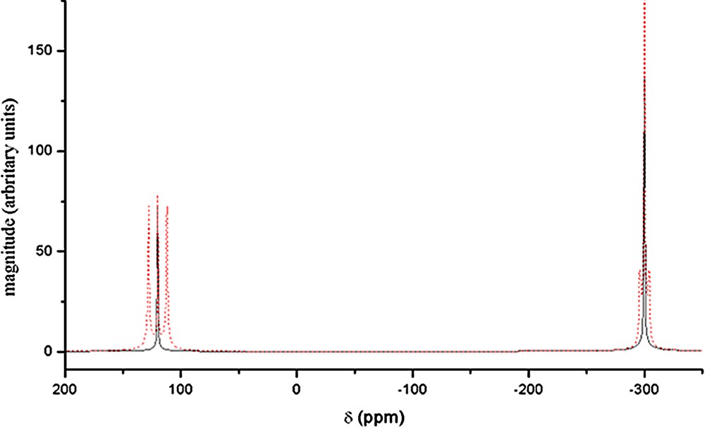
Simulated NMR spectrum of a doublet and triplet before (– – –) and after (__) analytical decoupling. Simulations made for magnetization with the following parameters: doublet, M0 = 200, T2 = 1 s, T2* = 0.6, J = 16; triplet, M0 = 300, T2 = 0.9 s, T2* = 0.5, J = 4. Analytical decoupling performed for k = 0.01. T = 1.44 s, F = 100, 200 echo delays.
Comparison of the magnitude ||S(0,k)|| for a doublet and a triplet for different values of k
| k | 0 | 0.01 | 0.1 | 0.2 | 0.3 | 0.4 | 0.5 | 0.6 | 0.7 | 0.8 | 0.9 | 0.95 | average |
| Doublet | 33.02 | 74.6 | 49.2 | 32.9 | 109.5 | 102.6 | 9.6 | 150 | 186 | 50.9 | 184 | 267 | 104 |
| Triplet | 122.9 | 120.6 | 6.7 | 132.6 | 83.4 | 77 | 233.12 | 5.19 | 369 | 46.6 | 359.9 | 11.2 | 131 |
| T/D | 3.72 | 1.62 | 0.14 | 4.03 | 0.76 | 0.75 | 24.3 | 0.035 | 1.98 | 0.92 | 1.96 | 0.042 | 1.26 |
One notes also that the average value of the signal for the different values of k gives a value compatible with a quantification with a higher intensity than for k = 0.01, but with a precision at 16% only. This last method would become more interesting than the analysis of S(t,k = 0.01) when the initial signal-to-noise ratio is poor. After an average for 12 values of k, the Gaussian noise would be divided by , whereas the signal would be at least 8% higher.
4 Conclusion
Analytical decoupling is a treatment of a signal detected after a spin-echo sequence that enables a decoupled spectrum to be obtained.
We have performed several magnetization simulations and transformed them so as to estimate the ability to quantify a signal after this treatment. We have shown that in the present conditions, demodulation of S(t,k) is inefficient for quantification. Instead, analytical decoupling can be employed for quantification by means of the function S(t,k), with k close to zero. Then, a deviation of less than 10% can be obtained for a spectrum with coupling constants between 1 and 16, a high signal-to-noise ratio, and a coefficient F set to 100. In the case of the analysis of a spectrum with a poor signal-to-noise ratio, this treatment would give an even noisier decoupled spectrum. There are two possibilities to maximise the signal-to-noise ratio in the final decoupled spectrum. The first one is to reduce the value of F. The second one is to calculate the average value of S(t,k) for different values of k between 0 and 1. The two possibilities deteriorate the robustness of the treatment and the deviations between the different signals due to the coupling suppression are higher. For the average spectrum, in the present case, the deviation is about 25%, instead of less than 10% previously, but with a significantly higher signal-to-noise ratio.
Complementary studies should be carried out so as to obtain precise results and keep at the same time a good signal-to-noise ratio in the final spectrum.