Neural network potentials for exploring condensed phase chemical reactivity

Axel Gomez; Miguel de la Puente; Rolf David; Damien Laage

doi:10.5802/crchim.315

Article de synthèse

Neural network potentials for exploring condensed phase chemical reactivity
[Potentiels de réseaux de neurones pour l’étude de la réactivité chimique en phase condensée]

Axel Gomez ¹ ; Miguel de la Puente ¹ ; Rolf David ¹ ; Damien Laage ¹

¹ PASTEUR, Department of Chemistry, École Normale Supérieure, PSL University, Sorbonne Université, CNRS, 75005 Paris, France

Comptes Rendus. Chimie, Online first (2024), pp. 1-17.

Résumés

Anglais
Français

Recent advances in machine learning offer powerful tools for exploring complex reaction mechanisms in condensed phases via reactive simulations. In this tutorial review, we describe the key challenges associated with simulating reactions in condensed phases, we introduce neural network potentials and detail how they can be trained. We emphasize the importance of active learning to construct the training set, and show how these reactive force fields can be integrated with enhanced sampling techniques, including transition path sampling. We illustrate the capabilities of these new methods with a selection of applications to chemical reaction mechanisms in solution and at interfaces.

Les progrès récents dans le domaine de l’apprentissage automatique offrent des outils puissants pour explorer les mécanismes réactionnels complexes en phase condensée par des simulations réactives. Dans cette revue, nous décrivons les principaux défis associés à la simulation de réactions en phase condensée, nous présentons les potentiels par réseaux de neurones et détaillons comment ils peuvent être entraînés. Nous soulignons l’importance de l’apprentissage actif pour construire l’ensemble d’entraînement, et nous montrons comment ces champs de force réactifs peuvent être intégrés avec des techniques d’échantillonnage amélioré, y compris l’échantillonnage des chemins de transition. Nous illustrons les capacités de ces nouvelles méthodes par une sélection d’applications aux mécanismes de réactions chimiques en solution et aux interfaces.

Métadonnées

Reçu le : 2024-01-31
Révisé le : 2024-04-17
Accepté le : 2024-05-14
Première publication : 2024-06-18

DOI : 10.5802/crchim.315

Keywords: Chemical reactivity, Machine learning, Molecular simulations
Mot clés : Réactivité chimique, Apprentissage machine, Simulations moléculaires

Affiliations des auteurs :

Axel Gomez ¹ ; Miguel de la Puente ¹ ; Rolf David ¹ ; Damien Laage ¹

¹ PASTEUR, Department of Chemistry, École Normale Supérieure, PSL University, Sorbonne Université, CNRS, 75005 Paris, France

Licence :

CC-BY 4.0

Droits d'auteur : Les auteurs conservent leurs droits

@article{CRCHIM_2024__27_S5_A4_0,
     author = {Axel Gomez and Miguel de la Puente and Rolf David and Damien Laage},
     title = {Neural network potentials for exploring condensed phase chemical reactivity},
     journal = {Comptes Rendus. Chimie},
     publisher = {Acad\'emie des sciences, Paris},
     year = {2024},
     doi = {10.5802/crchim.315},
     language = {en},
     note = {Online first},
}

TY  - JOUR
AU  - Axel Gomez
AU  - Miguel de la Puente
AU  - Rolf David
AU  - Damien Laage
TI  - Neural network potentials for exploring condensed phase chemical reactivity
JO  - Comptes Rendus. Chimie
PY  - 2024
PB  - Académie des sciences, Paris
N1  - Online first
DO  - 10.5802/crchim.315
LA  - en
ID  - CRCHIM_2024__27_S5_A4_0
ER  -

%0 Journal Article
%A Axel Gomez
%A Miguel de la Puente
%A Rolf David
%A Damien Laage
%T Neural network potentials for exploring condensed phase chemical reactivity
%J Comptes Rendus. Chimie
%D 2024
%I Académie des sciences, Paris
%Z Online first
%R 10.5802/crchim.315
%G en
%F CRCHIM_2024__27_S5_A4_0

Axel Gomez; Miguel de la Puente; Rolf David; Damien Laage. Neural network potentials for exploring condensed phase chemical reactivity. Comptes Rendus. Chimie, Online first (2024), pp. 1-17. doi : 10.5802/crchim.315.

Version originale du texte intégral (Proposez une traduction )

1. Introduction

The elucidation of reaction mechanisms is at the heart of chemistry. A mechanism identifies a molecular pathway involving a series of successive structures explaining the chemical reorganization caused by a reaction. Determining the mechanism, the order in which the elementary changes occur, and which of them causes the rate-limiting energy barrier is essential to guide the work of chemists to control reactivity and act on it, e.g., by catalyzing a reaction step. Organic physical chemists have achieved remarkable successes and determined the mechanisms of fundamental reactions such as nucleophilic substitutions and Diels–Alder reactions [1, 2, 3, 4]. This was obtained via a combination of approaches, including for example, linear free energy relationships, substituent effects and isotopic effects on the rate constant [3, 4]. However, these experimental approaches provide only an incomplete and often ambiguous description of the mechanism. In addition, it is well appreciated that reaction mechanisms as drawn in chemistry textbooks are largely idealized and that reactions actually proceed along pathways which can significantly deviate from these simplified representations. An in-depth determination of reaction mechanisms, taking into account path variability, would therefore be desirable, but remains almost inaccessible experimentally.

Numerical simulations appear as a perfectly suited technique for the determination of reaction mechanisms, since they naturally provide the desired atomic resolution. However, simulations face multiple challenges when it comes to modelling chemical reactivity in condensed phases such as liquids, solid/liquid and vapor/liquid interfaces, and biochemical environments. We now describe four of these challenges.

The first computational difficulty is that chemical reactions typically involve the breaking and making of covalent bonds, which imply electronic structure rearrangements. The mechanical description of molecular energies provided by classical force fields with fixed bond patterns and fixed partial atomic charges is therefore not adequate, and the electronic structure should be determined along the reaction pathway by solving (approximately) the electronic Schrödinger equation at every step. Density functional theory (DFT) is nowadays a method of choice for chemists, since it offers an attractive balance between cost and accuracy [5].

However, a second difficulty arises from the large size of the systems of interest. Studying chemical reactivity typically requires very large molecular systems, since one should not only describe the reaction partners, but also the surrounding solvent molecules which impact the properties of the reagents. This implies that systems of at least hundreds or thousands of atoms should be included in the electronic structure calculation. While very good DFT functionals can be used for small molecular systems (with a few tens of atoms), larger systems induce very high computational costs.

A third challenge is that reaction equilibrium constants and reaction rate constants are governed by differences in free energies, respectively between reactant and product and between reactant and transition state, and not by potential energies. At ambient temperature, the entropic contribution to these free energies can thus be important, and determining these free energies requires an extensive sampling of the configurational space. This therefore imposes long (more than nanosecond-long) molecular dynamics simulations propagated with forces obtained from DFT calculations. This implies that the costly electronic structure calculations must be repeated millions of times. Pioneering studies using ab initio (i.e., DFT-based) molecular dynamics [6] have already provided valuable insight in a broad range of chemical reaction mechanisms, showing the potential of this approach (see, e.g., Refs [7, 8, 9, 10, 11, 12]). However, they often face limitations in the system size and in the trajectory length, and therefore in the precision on the computed free energies. Systems of a few hundreds of atoms simulated for a few hundreds of picoseconds typically require millions of CPU hours on a single computer (i.e., more than a hundred years) and remain little practical despite the availability of parallel computing architectures.

The accessible simulation times thus remain much shorter than typical reaction times. It is therefore very unlikely that a trajectory initiated in the reactant state will spontaneously cross the reaction free energy barrier(s) to form the product during the available simulation time. Elucidating the reaction mechanism thus imposes to force the reactants to move along the reaction coordinate. However, this requires identifying the reaction coordinate and this is a fourth challenge. While chemical intuition can be used for simple reactions like acid/base proton transfers, for complex mechanisms determining the reaction coordinate is precisely what chemists try to do and for which the assistance of simulations is requested. Enhanced sampling methods have been proposed to identify pathways on complex energy surfaces [13, 14, 15, 16, 17], but they require extensive simulations, and have so far been mostly used with classical force field descriptions of the energies and forces (e.g., for protein folding) and very little for chemical reactions because of their prohibitive computational cost.

Recent developments in machine learning now provide a solution to all these challenges [18, 19, 20]. Among the many machine learning approaches that have been applied to interatomic potentials, deep neural networks have been particularly successful [18, 19, 20]. In this paper, we describe how these recent developments now allow training neural networks which provide the energies and forces traditionally obtained from an expensive resolution of the Schrödinger equation, and how they can be combined with enhanced sampling methods to determine the mechanisms of complex reactions in condensed phases. We introduce the structure of neural network potentials in Section 2, then we describe how they are trained in Section 3, and present applications to chemical reactions in Section 4. We finally offer some concluding remarks in Section 5. We emphasize that our goal is to provide a tutorial review and we will often direct the reader to excellent, more specialized reviews on the specific aspects that will be discussed.

2. Neural network potentials

As described in the introduction, the first challenge in performing molecular simulations of a reactive system is to obtain the energies and forces. This can be done either “on-the-fly” or a priori.

In Born–Oppenheimer ab initio molecular dynamics [21, 9], the Schrödinger equation is solved “on-the-fly” for the valence electrons at a given electronic structure level (typically DFT) to obtain the forces on the ions (formed by the nuclei and core electrons) in a given configuration and to propagate the trajectory to the next step. One advantage is that forces are only determined for configurations which are visited by the trajectory. However, a limitation is that forces must be evaluated at every step of the simulation, and the resulting computational cost has so far limited the size of the systems and the length of the trajectories. Reactive extensions of classical force fields [22, 23] have also been used: because they are parametrized to describe some pre-defined chemical reaction, they do not require expensive electronic structure calculations. While these approaches have been successful for some combustion reactions and enzymatic reactions, they remain less accurate than ab initio approaches and can exhibit parameterization biases.

Another approach for the calculation of forces and energies relies on the a priori calculation and fitting of the potential energy surface (PES) on which the system is evolving. While this approach has been successfully used for gas phase reactions and spectroscopy [24], it was for some time limited to small systems, due to the complexity of fitting a highly multidimensional PES. However, the idea of fitting the PES of a molecular system around a reduced number of configurations of known energy (computed at the given reference level of theory) to gain access to entire regions of the PES with a reduced computational cost but comparable accuracy has known a growing interest for several decades [25, 26, 27, 18, 28]. The mapping of atomic configurations to the PES was initially performed through analytical functions [25, 24], but this approach was limited to low dimensionality problems. Modern machine learning (ML) techniques are ideal tools to perform these mappings in more complex situations, and have been used since the early 2000s in the context of computational chemistry [27, 18]. Two very successful ML tools to fit high-dimensional PES of molecular systems in the condensed phase are kernel-based regression methods (including, e.g., (symmetric) Gradient Domain ML [29, 30] and Gaussian Approximation Potentials [31]) and neural network (NN) based methods [18, 32, 33, 34, 35, 28]. The advantages and limitations of each family of methods have been discussed in great detail in excellent reviews [19, 36]. Very briefly, the choice of a given method typically depends on the systems and objectives of the study. Kernel-based regression methods present a series of advantages: they tend to outperform NN-based methods in the low-data regime and the lower architecture complexity makes them more easily interpretable (noticeably, Gaussian Approximation Potentials [31] are able to provide analytical uncertainties on predicted quantities). However, NN-based methods are generally more efficient in the high-data regime and tend to present higher prediction efficiencies and scaling with, e.g., system size and number of chemical elements.

Here we focus on the applications of NN-based techniques to chemical reactivity in the condensed phase. Several approaches have been proposed, including, e.g., the SchNet architecture [34], ANI [37], and the DeepPot-SE scheme [32, 33, 20]. Most of them rely on the High-Dimensional NN (HDNN) concept introduced by Behler and Parrinello [18]. HDNN provides an elegant solution to one of the main difficulties in mapping the nuclear configurations of atoms to the PES with NN. In earlier implementations, because many of the PES symmetries (e.g., invariance upon translation, rotation, permutation of identical atomic species) were not directly encoded in the usual representations of configurations via Cartesian or internal coordinates, these invariances had to be learned directly by the NN [26] which limited their accuracy and scalability with system size. In HDNN, the total energy of the system is decomposed into atomic contributions E =∑ _i∈ atoms E_i, which are predicted by a single NN per atomic species. This decomposition makes the energy invariant upon permutation of the coordinates of identical atomic species and provides a NN potential (NNP) model (the set of NN for each individual species) that can in principle be used to study systems with an arbitrary number of atoms. The other invariances of the PES can then be either learned directly from the nuclear positions (generally in the local frames of reference of every atom) in what are sometimes called end-to-end NNPs [33], or encoded in human-designed descriptors of the atomic configurations including, e.g., symmetry functions [38]. This total energy decomposition assumes that the atomic energy depends only the atomic environment within a finite range, but long-range effects important for, e.g., electrostatics can be considered separately and we will return to this point at the end of this section. The general workflow of a NNP for the prediction of molecular energies and forces is presented in Figure 1.

Figure 1.
Schematic representation of a NNP workflow to map the atomic configurations of a system to the PES. In a given configuration, a local environment matrix is defined for every atom $𝓡^{i}$ : the latter contains the chemical element and the positions in the atomic frame of reference of every neighboring atoms within a given cutoff distance. These local environments are transformed (either manually or through the use of embedding NN) into descriptor vectors $𝓓^{i}$ , which preserve the invariances of the PES. These descriptors are then transformed into atomic energies E_i by fitting NN (one per type of atomic species), which yield the configuration energy $E ({{\vec{r}}_{i}})$ after summation. This energy can be analytically differentiated to obtain the atomic forces ${\vec{F}}_{i}$ needed to propagate MD. The prediction error on both of these quantities is used to adjust the parameters of the fitting (and, if needed, those of the embedding) network during backpropagation.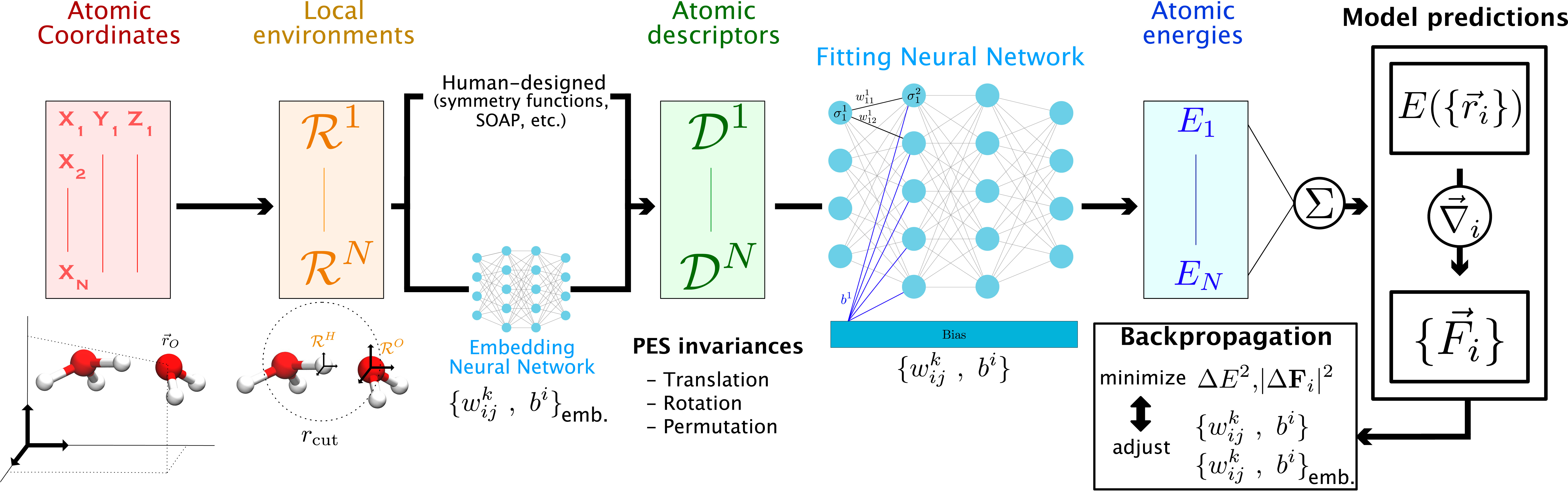

In the following, we focus on the implementation of end-to-end NNPs provided in the Deep Potential - Smooth Edition (DeepPot-SE) model [33], within the DeePMD-kit package [32, 20]. This choice is motivated by the successful applications of this approach to chemical reactions recently obtained in our group [39, 40, 41] and because it presents a good trade-off between prediction accuracy and computational efficiency [42]. However our discussion remains general since our conclusions could have been obtained with other families of end-to-end NNPs. This model has been presented in detail elsewhere [33, 20], and here we only summarize its most important features, some of which are shared with other NNP families. The philosophy of the DeepPot-SE scheme is to limit human intervention as much as possible in the construction of the PES model. The complex relation between the local atomic environment and the energy is therefore learned through intermediary embedding NNs that map the coordinates of the system onto non-linear descriptors, produced as the output layer of the embedding NN. These descriptors are then provided as inputs to the fitting NNs that predict the atomic energies (see Figure 1). In order to minimize the amount of information that needs to be learned by the NNPs, the descriptors of every atom are usually built by the embedding NNs from the positions of the other atoms within its local frame of reference (which is already a translationally invariant representation). Furthermore, because the energy of a given atom is mostly determined by its local environment, only the coordinates of atoms within a given cutoff distance (typically 6 Å) are used as input of the embedding NN. While this is an approximation to which we will return, this has the key advantage of limiting the computational cost and ensuring that the model can be used for systems of arbitrarily large sizes.

The parameters of both NNs (called weights and biases) are simultaneously optimized during the training process: this consists in the minimization of the following loss function L defined as the sum of mean square errors (MSE) of the NNP predictions on several target quantities:

L (p_{E}, p_{f}) = \frac{p_{E}}{N} 𝛥 E^{2} + \frac{p_{f}}{3 N} \sum_{i} | 𝛥 F_{i} |^{2}

(1)

N is the number of atoms in the system and 𝛥E² and |𝛥F_i|² are the MSE on the energy and on the atomic forces. An additional term involving the system virial can be introduced in the loss function, and is typically employed for solid state systems. Since in practice it has little impact for reactive models in the liquid phase we remove it here for clarity reasons. The prefactors p_E and p_f determine the relative importance of each target quantity; they are chosen by the user and typically evolve during the minimization procedure following the adaptive learning rate [43]. During this minimization, the MSE are computed from the differences between the target quantity predicted by the NNP and the reference value for a random subsample of configurations (often called a batch) and the weights and biases of both NNs are modified by backpropagation. The atomic forces are computed by differentiation of the predicted total energy with respect to the atomic coordinates, which imposes that this quantity vary smoothly enough to always be differentiable. This is enforced in the Smooth-Edition scheme by applying weighting functions (e.g., cosine [32] or polynomial [20] functions) to the radial components of the local atomic coordinates that are used to build the descriptors in the embedding step.

In practice, despite the end-to-end philosophy of the DeepPot-SE scheme, many hyperparameters of the model need to be chosen by the user. These include, e.g., the number of layers and neurons of both NN, the prefactors of the target quantities in the loss function, the batch size, and the total number of training iterations. Systematic grid search procedures can be used to determine these hyperparameters. However, this can require large amounts of validation data. Fortunately, the NNPs performances have been found to remain robust over a reasonable range of these hyperparameters. This implies that it is often possible to use similar sets of hyperparameters for training NNPs on different chemical systems.

We quickly present typical sets of hyperparameters that we have successfully used in our group to train NNPs for reactive systems in the liquid phase. For the NN architectures, three hidden layers of some tens of neurons for the embedding network and four hidden layers of some hundreds of neurons for the fitting network are enough to yield NNPs of the same quality as that obtained with larger architectures which induce larger computational costs. For the prefactors of the loss function components, we have found that using a much larger prefactor for the atomic forces than for the energies at the beginning of the training procedure typically yields NNPs that are more stable during the MD simulations. We typically employ p_f and p_E prefactors that range from approximately 1000 and 0.01 respectively at the beginning of the training procedure to 1 and 0.1–1 at the end. The total number of training iterations can be set between some hundreds of thousands to some millions depending on the training set size (the number of reference configurations used for the training) and batch sizes below 5 all give comparable NNPs. Finally, the learning rate used for the parameter optimization is adapted during the training procedure and we have found that limiting values of 1 × 10⁻³ and 1 × 10⁻⁸ at the beginning and at the end of the training procedure give satisfactory results.

As described above, the DeepPot-SE scheme corresponds to what are sometimes called “second generation” NNPs [36], which currently are the most commonly used NNPs to study reactivity in the liquid phase. The main limitation of this NNP generation is the absence of explicit long-range effects in the construction of the descriptors, which can lead to unphysical behaviors in situations where these effects can significantly affect the energy of a configuration (most noticeably at interfaces in the presence of charges). However, we stress that long-range interactions are present in the reference energies and forces used for the training, and are therefore described in a mean-field manner. Adding configurations with long-range interactions to the training set can be enough to correctly reproduce the physics of such systems, as these long-range effects can be indirectly learned by the NNs [44]. Long-range effects can also be explicitly included in the NNP description of the system in what are called “third generation” NNPs [36] (which have been implemented with the DeepPot-SE model in the DeePMD-kit package [45]). However, these have so far had limited applications to realistic reactive systems and we will therefore focus on examples of applications of the “second generation” DeepPot-SE models.

3. Training set construction

Neural network potentials exhibit high accuracy in predicting energies and forces for configurations closely resembling those in their training set. However, deviations from these trained configurations lead to a rapid deterioration in the prediction accuracy of the neural network model—a challenge known as generalization performance [43]. The careful selection of configurations to be included in the training set is therefore critical in determining the quality of the NNP. This section outlines systematic approaches aimed at enhancing the accuracy of NNP for structures encountered in chemical reactions, with a specific focus on active learning procedures that iteratively refine NNP accuracy.

Identifying and generating relevant chemical structures for the training set is a formidable task, due to the overwhelming dimensionality of the chemical space. Several approaches can be followed. The first one is that adopted by several on-going efforts to generate general-purpose NNPs aimed at providing a universal force-field [37]. The training sets of these NNPs are typically parts of existing very large structure datasets of realistic synthesizable molecules. One such example is the publicly available GDB-11 dataset [46], which contains all molecules made of up to 11 atoms of carbon, nitrogen, oxygen or fluorine and includes 26.4 million distinct structures. However, this approach is not practical for reactivity in condensed phase for two main reasons. The first one is that solvent arrangements need to be included in the configurations, which considerably increases the possibilities to be considered. Different strategies have been proposed to overcome this limitation and generalize NNPs trained on small systems to be transferable to larger molecular systems, including the condensed phase [47, 48, 49]. For example, in the same fashion as hybrid QM/MM techniques, hybrid NNP and molecular mechanics (NNP/MM) simulations are being developed to treat a solute by machine learning models while the solvent is described with a classical force-field [50, 51]. However, these setups cannot easily describe reactions that involve solvent molecules. The second very important difficulty arises because the study of chemical reactivity requires to include high-energy transition-state geometries, which are not present in databases of stable structures.

Simulating chemical reactions in condensed phases therefore requires the specific training of the NNP on configurations that are representative of the region of phase space explored during the reaction. The training set should contain all kinds of structures that will be encountered during the reactive simulations, including typical configurations of the reactants, transition states and products, but also intermediate structures visited along the reaction coordinate.

The a priori identification of all relevant configurations to be included in the training set, e.g., from an ab initio MD simulation, is usually not possible. One therefore uses an iterative approach to progressively enrich the training set and systematically improve its prediction accuracy. Such an approach was for example implemented in the deep potential generator (DP-GEN) [52].

We now describe this active learning strategy combined with a query by committee [53] estimation of the NNP quality. As described in Figure 2A, one starts from a small training set including configurations that are representative of limited regions of the phase space, typically stable reactant configurations easily sampled in short DFT-based MD simulations. A few hundreds of configurations with energies and forces at a selected reference level of theory (DFT with a hybrid functional, for example) typically constitutes a valid initial training set. Here it is important to select uncorrelated structures in order to maximize the amount of information present in the dataset. Based on this initial set of configurations, a first approximate NNP can be trained.

Figure 2.
Concurrent learning scheme. (A) Iterative exploration of the phase space until convergence. The relevant region of phase space for the chemical reaction of interest is in dark gray. The black lines represent schematically a free energy surface. The part of configurational space known to the NNPs at each iteration is in green, the intermediate region that provides new structures to be added to the training set is in yellow. The red area corresponds to regions where the NNPs extrapolate significantly but that may be accessible during the exploration phase. (B) Training set construction algorithm. (C) NNPs committee evaluation test. The number of candidates, i.e. configurations selected to be labeled and added to the training set, decreases over iterations. A threshold value can be decided as an interruption criterion. (D) Correlation between the NNP predictions and the reference calculations, for example for energies or forces. (E) Schematic representation of a learning curve where the error on the training set and the test set are represented as a function of the number of data used for training.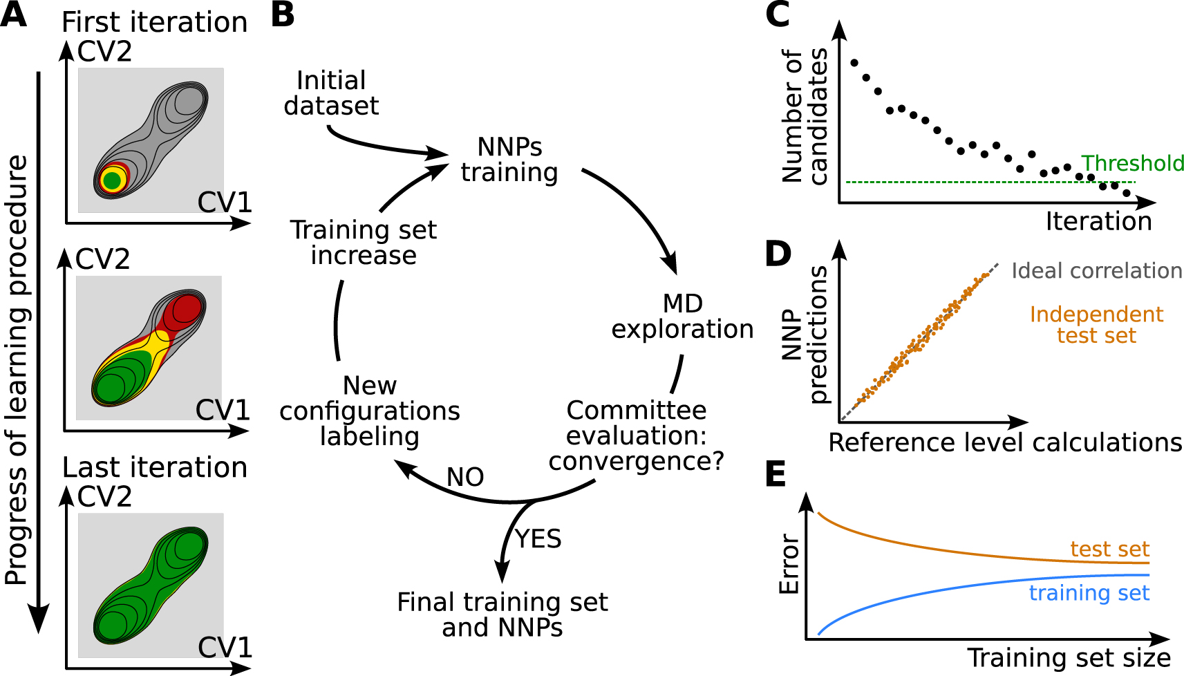

The next step is to discriminate between configurations whose forces and energies are properly predicted by the NNP and configurations which are unknown and poorly described. Contrasting the NNP prediction with reference DFT calculations would be extremely expensive. One therefore uses the query by committee approach [53] to estimate the quality of the prediction provided by the NNP. Several distinct NNPs are trained on the same training set but initialized with different random parameters. After training, their predictions all converge to a similar answer in regions where they are properly optimized, but significantly differ for configurations far from these in the training set. This deviation between NN predictions is therefore exploited to identify which configurations are already known by the NNP model and which ones are unknown and should be added to the training set. In our studies, three or more NNP models are typically trained on the same training set at each step of the iterative training procedure.

An additional advantage of this concurrent learning approach is that it greatly mitigates the risk of instabilities recently found [42] for models trained with different approaches and for which the average values of different observables (including, e.g., radial distribution functions) fluctuate unphysically during the molecular dynamics trajectory. The iterative nature of the training set construction, guided by collective variables based on chemical knowledge, ensures that the chemical space accessible to the system is sampled systematically, which greatly reduces the risks of encountering configurations leading to instabilities during production. Furthermore, monitoring the deviation between the committee of NNPs during the molecular dynamics trajectory allows an “on-the-fly” detection of these instabilities, which might not be directly detectable from the model performance over a possibly incomplete test set.

At each iteration of the active learning, the ensemble of NNPs is then used to propagate short MD trajectories. The goal is to explore the phase space around the region of the training set, in order to identify configurations where the NNP prediction is poor and which should thus be added to the training set. The maximal deviation on the atomic forces computed by all models serves as a proxy to measure whether the configurations are already known or should be added to the training set to improve it. MD configurations that are very similar to a subset of the training set will exhibit a low maximal deviation on forces, typically of the order (or below) of 0.1 eV⋅Å⁻¹. Frames containing new structures will be associated to a large maximal deviation on forces. New configurations to be added to the training set are usually selected at the border between the region already included in the training set (Figure 2A, green region) and the unknown (see Figure 2A, yellow region). This corresponds to intermediate values of maximal deviation on forces, typically between 0.1 and 0.8 eV⋅Å⁻¹. In this region, the NNP model is not accurate but it does not completely fail or break. In the red area of Figure 2A, the committee of NNPs gives a very large maximal deviation. This corresponds to configurations that, although accessed during the exploration phase, might be highly non-physical and where the NNPs cannot be trusted at all. The new structures with intermediate deviations, called candidates, are usually sub-sampled to ensure a proper decorrelation, before being labeled at the same reference level as the training set and added to it. The improved dataset is used for training new NNP models for the next iteration of the procedure (Figure 2B). As illustrated schematically in Figure 2A, each iteration pushes further the limits of the region of configurational space that is properly described by the NNP.

A key feature of the training set is that it should cover all the structures to be visited during the subsequent simulations. For chemical reactions, this implies that unbiased MD simulations during the active learning iterations are not adequate. Typical barriers between the reactant and product basins are significantly larger than the thermal energy k_B T, where k_B is the Boltzmann constant and T the temperature, and the transition state region will not be explored spontaneously. The active learning explorations are therefore performed with enhanced sampling techniques, including, e.g., metadynamics [13], on-the-fly probability enhanced sampling (OPES) [17] or umbrella sampling [54], or at elevated temperatures to enhance the sampling. The choice of the enhanced sampling technique—and of the relevant collective variables when applicable—is crucial for an efficient exploration step for cases where the free energy landscape features larger than thermal energy barriers. In addition, if the NNP is developed for path integral MD (PIMD) [55, 56] simulations for an explicit description of nuclear quantum effects, the training set should include typical configurations of the path integral beads, since such simulations evaluate the forces on the beads. Alternatively, nuclear quantum effects can also be learned directly in the framework of machine-learned centroid molecular dynamics schemes [57].

The iterative enrichment of the training set is stopped when the quality of the NNP is considered to have converged. The number of configurations that are retained to be labeled and added to the training set after an exploration phase is a good indicator of the convergence. If less than a user-specified number of structures are pointed out by the committee of neural networks, then it can be assumed to be converged (Figure 2C). A converged concurrent learning process can generate thousands or tens of thousands configurations for the training set, depending on the chemical complexity of the system.

One should then validate the quality of the NNP. There is no absolute condition to assess the reliability of the optimized NNP but a collection of metrics that confirm the quality of the model is usually deemed satisfactory [58]. The NNP validation is assessed on an independent test set of configurations. The latter includes configurations sampled within the region of configurational space of interest and whose energies and forces are labeled at the reference level of theory. This validation set is a separate dataset that is not included in the training set. The NNPs are used to predict energy and forces of the configurations in the test set and the predictions are compared with the reference values (Figure 2D). The correlation is considered to be acceptable when the average prediction errors on forces are typically below 0.1 eV⋅Å⁻¹. This is complemented by the analysis of the learning curve, which represents a measure of the relative error, e.g., the root-mean squared NNP error on the energy or on the forces divided by the standard deviation of the reference data, both on the training set and on the independent test set as a function of the size of the training set used (Figure 2E). For small training sets, prediction errors are typically much lower on known configurations (included in the training set) than on unknown ones (such as those in test sets), which is known as overfitting [36]. This difference of performance usually results from an imbalance between the model complexity (featuring too many optimizable parameters) and the amount of information present in the training set. It can thus be monitored while the training set size increases by comparing the prediction errors over the training set and over an independent test set. As the amount and diversity of data included in the training set increase, the gap between the prediction errors on training and test sets should decrease (see Figure 2E). This is typically referred to as a decrease in overfitting or, equivalently, an improvement of the generalization performance of the model.

Practically, the concurrent learning procedure depicted in Figure 2B is performed via a combination of software: one to train the NNP, for example DeePMD-kit [32], a MD engine interfaced with the NNP software to propagate MD simulations, which can be LAMMPS [59] for classical nuclei MD simulations or i-PI [60] for PIMD, optionally coupled with PLUMED [61] for enhanced sampling, and an electronic structure code for energy and forces calculation at the chosen reference level of theory, e.g., CP2K [62]. A series of scripts are needed to prepare the files and extract the configurations to be added to the training set. For some simple applications, this procedure has been implemented in the DP-GEN software [63]. For more complex reactions which require, e.g., several enhanced sampling techniques or the explicit consideration of nuclear quantum effects, we have developed our own suite of scripts (https://github.com/arcann-chem/).

4. Applications of NNP for reactivity

4.1. Brief overview of recent applications

The application of NNPs to chemical reactivity in solution and in materials is expanding extremely rapidly. For example, they have been successfully used to study proton transfer reactions, including water self-dissociation in the bulk [64] and at the air–water interface [40] and proton transport in porous materials [65]. NNPs have also been applied to heterogeneous catalysis reactions, including water dissociation on TiO₂ surfaces [66, 67, 68, 69] and ammonia decomposition [70]. They have been used to investigate the mechanisms of chemical reactions, such as Diels–Alder cycloadditions [71], prebiotic amino acid synthesis [72], urea decomposition [73], and different reactions relevant to atmospheric chemistry [74, 75]. They have even been extended to the very complex reaction schemes involved in combustion [76, 77]. While we cannot provide a comprehensive review of these applications, in the following we illustrate the capabilities and limitations of this method for a number of reactions that have been studied in our group.

4.2. Application to a simple reaction

We first describe how NNPs have been applied to study the dissociation of formic acid in water and at the air–water interface [39]. Extensive experimental and simulation studies had concluded that simple acids including formic acid experience a change in their acidity between the bulk solution and the air–water interface. This question attracted an important interest because of the major implications for the description of chemical reactions at the surface of atmospheric aerosols. However, both experiments and simulations led to contrasted results, reporting both acidity enhancement and reduction for the same acid, depending on the technique being used.

For simulation studies, the challenge is twofold. First, the simulations have to be able to describe the dissociation reaction, so that DFT-based molecular dynamics simulations would be typically used. Second, in order for the comparison between the acidity in the bulk and at the surface to be conclusive, the uncertainties on the acid dissociation free energies should be much smaller than the difference between the dissociation free energies in the bulk and at the water-interface. This requires the careful convergence of these calculations, and therefore long simulations. However, the computational cost of DFT-based simulations typically imposes strong limitations on the trajectory length, and thus on the precision of the calculated free energy difference.

We therefore trained a NNP to describe the dissociation of formic acid both in the bulk and at the air–water interface, at the BLYP-D3 level of theory. The training set was constructed iteratively as described above and includes both bulk and interface environments, and configurations at different stages of the dissociation reaction. Here the reaction mechanism is known and can be described with a simple reaction coordinate, that we chose to be the hydrogen coordination number around the acidic oxygen atom of formic acid, which decreases from 1 in the acidic form to 0 in the conjugate base formate ion. Biased sampling along this coordinate was used to generate training set configurations. We note that while the NNP does not include long-range interactions because of its short-range cutoff, long-range interactions are accounted for in the reference energies and forces calculated for the training set configurations, so that long-range interactions between charged species for example are described by the NNP in a mean-field manner.

Typical dissociation reaction free energy profiles are shown in Figure 3 in the bulk and at the air–water interface. The thickness of each curve reports the 95% confidence interval on the free energy, which shows the excellent convergence provided by our long simulations. These calculations could unambiguously reveal that formic acid dissociation is less favorable at the air–water interface than in the bulk, in agreement with vibrational sum frequency generation spectroscopy and with X-ray photoemission spectroscopy [39]. We could then use these dissociation free energy profiles as the starting point of a model to predict the dissociation free energy based on the respective solvation free energies of the reaction partners (formic acid and water reactants, formate ion and hydronium products). This approach was also extended to the dissociation of the strong inorganic nitric acid in the bulk and at the interface [39]. In a subsequent study, we followed a similar approach to study the self-dissociation of water which governs the pH of neat water, and we showed how it is affected at the air–water interface, and how this determines the pH of small aqueous aerosols [40].

Figure 3.
Formic acid dissociation free energy profile in the bulk (blue) and at the air–water interface (red) along the hydrogen coordination number around the acidic oxygen atom of formic acid [39].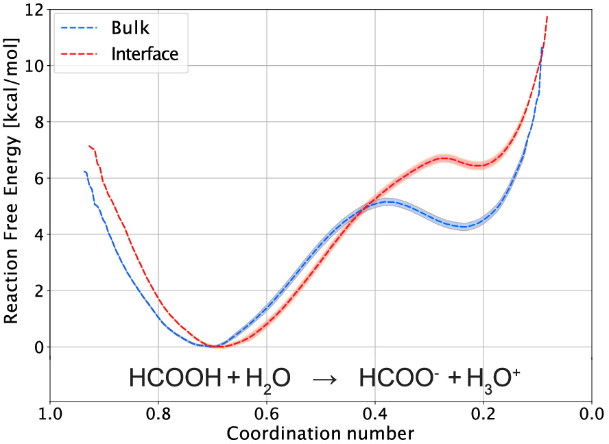

4.3. Application to a more complex reaction

While the aforementioned examples highlight the potential of NNPs to study chemical reactivity in the bulk and at interfaces, the cases described so far involve simple single-step reactions, with a well-defined reaction coordinate. However, many reactions of interest are far more complex. They can involve multiple intermediates and transition states, a series of concerted or sequential steps, and several competing pathways leading to the same or to different products. Well-known examples of such important but complex reactions are the Wittig reaction, the aldol condensation, and the Michael addition, for which changing the conditions can lead to different products, and the S_NAr reactions and amine protection–deprotection reactions which involve multiple steps [78].

The importance of the proper identification of the reaction coordinate is illustrated by the model free energy surface in Figure 4A. For the reaction transforming the reactant A into the product B, two transition states TS₁ and TS₂ are revealed when the free energy surface is represented along the two collective variables (CV1 and CV2). However, if the CV2 coordinate is ignored, these two pathways cannot be distinguished and the two transition states will appear as a single saddle point in the one-dimensional profile along CV1 (Figure 4B). If the two transition state structures have different entropic properties, they will be affected differently by temperature, changing the relative importance of the two pathways, and this could not be understood by considering the profile along CV1 only. In addition, a proper sampling of the two transition state structures is likely difficult if the CV2 coordinate is not considered explicitly.

Figure 4.
(A) Model free energy surface along CV1 and CV2. The gray square represents the two minima (A and B). The two minimum free energy profiles are represented with black and white solid lines. The two transition states are represented by a black triangle and a white square. The path ensembles are represented by the blue and green lines. (B) Free energy profiles of the same model free energy surface represented along the s reaction coordinate for both the blue and green paths and along CV1 when CV2 is not considered explicitly (dashes). (C) Scheme of a shooting move in Transition Path Sampling, with the initial path (solid gray line), the shooting point (purple circle), the new path (dashes for the forward time propagation and dots for the backward time propagation).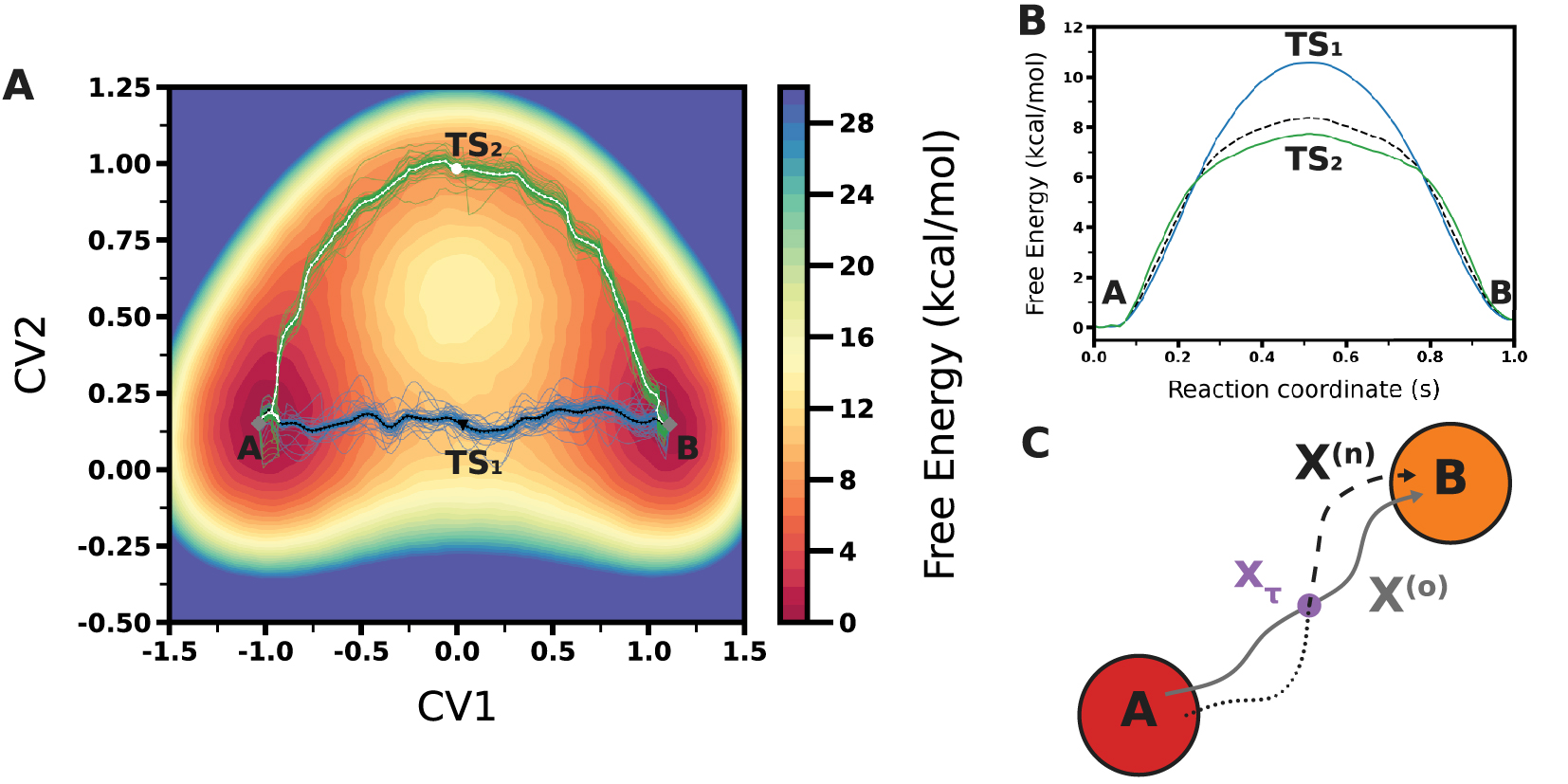

A number of methods have been proposed to identify reaction pathways on complex energy surfaces. When a very limited number of coordinates is to be considered, traditional multidimensional free energy surface calculations using umbrella sampling or metadynamics can be used, and the pathway can be determined a posteriori. When a larger number of coordinates is involved, these methods become impractical because of the necessary computational effort, and other methods which do not require computing the full dimensional free energy hypersurface have been proposed. An attractive approach is provided by the adaptive string method (ASM) [79] which focuses on the minimal free energy path (MFP) and determines the free energy surface only in the vicinity of the reaction path. Based on the string method [80], this method considers a string that spans from A to B. This string is then optimized iteratively, moving on the free energy surface towards the MFP. When convergence is reached, the string is then used to identify the path collective variables (parallel s and transverse z) [81] corresponding to the MFP, to determine the reaction pathway, and to calculate the free energy profile with the reaction transition states and intermediates. While this method can consider a large number of collective variables (typically from 2 to 10), it remains critical for the quality of the final result to include all relevant coordinates. Considering the model surface in Figure 4A, both CV1 and CV2 should be considered to identify the two pathways, and a string defined with CV1 but not CV2 would probably only identify the blue reaction path.

It is therefore interesting to consider other methods which do not require any a priori selection of coordinates in the generation of reaction pathways. One such very popular method is transition path sampling (TPS) [82, 83, 14, 15, 84]. TPS only requires a set of conditions that define the starting state A and the ending state B, together with one pathway connecting A and B. The latter does not need to be the minimum free energy path, and it is typically generated by high temperature or biased simulations. Using a Monte Carlo approach, TPS then iteratively generates the statistical ensemble of pathways connecting A and B. TPS is described in detail in excellent reviews [15, 14, 84, 85] and we only summarize its simplest form. The initial path (X^(o)) is discretized in L snapshots, x_i, with $0 \leq i < L$ . One snapshot $x_{𝜏}^{(o)}$ is selected, and a shooting move is performed by propagating a new trajectory forward and backward in time from this snapshot. One considers if this new trajectory connects A and B, and it is accepted according to a Metropolis criterion. One then performs another iteration, selecting a snapshot either from the new path (X⁽ⁿ⁾) if it has been accepted or from the old path (X^(o)) if it has been rejected, until an adequate number of decorrelated paths are obtained. TPS has been further extended to more complex situations [86, 87, 88, 89, 85]. TPS therefore provides the ensemble of reaction pathways, with the important advantage that they are generated from unbiased trajectories and thus with the true dynamics. The transition path ensemble can then be a posteriori projected on a selection of collective variables (CVs) to identify the most relevant ones and define a simplified reaction coordinate (but this choice does not affect the transition path generation). It can further be used for a committor analysis, to identify the transition state location, and the ensemble of pathways can be used to determine the free energy profile [90]. We note that other related techniques including transition interface sampling [91, 92] and forward flux sampling [93, 94] are also available to explore the free energy landscape (see, e.g., the review in [95]).

TPS has been extensively used for biophysical phenomena occurring on rough free energy surfaces, including protein folding, but it remains a computationally demanding technique due to the very large number of trajectories required. While TPS has been successfully applied to some chemical reactions [96, 97, 98], the cost of propagating these many trajectories with a description that accounts for chemical reactions, i.e., typically DFT-based MD, has so far hindered its broad application to reactivity.

Combining TPS and NNP therefore provides a promising approach to explore chemical reactivity in complex systems. In the following, we describe a study performed in the group [41] where we used the TPS implementation of OpenPathSampling [99, 100] together with the OpenMM [51] MD engine interfaced with DeePMD-kit [32, 20] and the biased sampling tools provided by PLUMED [61].

We present the application of this method to study the formation of a peptide bond. The condensation of an amine and a carboxylic acid to yield an amide is a key step in the formation of polypeptides, since the latter are polymers of amino acids linked together by peptide bonds. In addition, amide formation is one of the most common reactions in organic synthesis. In bulk aqueous solution, this reaction is extremely unfavorable. In living organisms, it is catalyzed by enzymes and in organic synthesis it is typically performed after activating the reactants, for example by replacing the carboxylic acid with an acyl chloride or an acyl anhydride. Understanding the mechanism of this reaction is therefore of great interest for organic synthesis, but also in the context of prebiotic chemistry.

The reaction involves several rearrangements: the formation of the C–N bond, the breaking of the C–O bond, and at least two proton transfers (see Figure 5). The sequence of these steps is not clear, and it has been a subject of debate since a mechanism (see Figure 5A) was proposed by Jencks in the late sixties [101, 102]. The mechanism is considered to start with the formation of the C–N bond, yielding a tetrahedral species (T^±) which has been proposed as either a long-lived intermediate or a short-lived transient structure [101, 102, 103, 104], followed by the cleavage of the C–O bond. Numerous theoretical studies have been published on this reaction, using a variety of methods ranging from gas-phase DFT calculations to QM/MM simulations, in order to investigate the mechanism and the role of the solvent [105, 103, 106, 107, 104, 108].

Figure 5.
(A) The amide formation mechanism proposed by Jencks for the aminolysis of acetate ester (with the nucleophilic amine in olive and the leaving group in violet). (B) The two pathways for peptide bond formation identified in our calculations: the general-base catalysis mechanism similar to Jencks’ proposal (path 1) and mechanism with no acid-base catalysis which is the most favorable one in pH-neutral conditions (path 2). The same color code is used for the reacting groups as in (A). (C) Transition path ensemble probability obtained from our TPS results for the peptide bond formation as a function of three CVs, respectively the 𝛥d = d_CO − d_CN difference of bond lengths, and the C_O,N hydrogen coordination numbers around O and N where the path 1 is represented in blue and path 2 in green. (D) Free energy profiles for the two pathways obtained by umbrella sampling along the path collective variable of each mechanism, represented with the same color code as in (C).

We first describe the training of the NNP. Following the active learning approach described above, we have constructed our training set iteratively, with reference energy and force calculations performed at the DFT-GGA level of theory (BLYP-D3). The final training set contains an ensemble of approximately 75,000 diverse configurations encompassing reactants, products, intermediates, and transition states, all solvated in a cubic box with 300 water molecules [41]. These reactive structures were sampled via enhanced sampling using multiple collective variables to describe the reaction, including 𝛥d = d_CO − d_CN, the difference in the lengths of the forming C–N bond (d_CN) and of the breaking C–O bond (d_CO), and 𝛥C = C_N − C_O, the difference in coordination numbers between the nucleophilic amine nitrogen and the leaving group oxygen with any hydrogen atom, which are “chemically intuitive” variables. Several additional collective variables, such as the protonation states of the solvent, were also used to ensure an even training of the NNP on all mechanisms proposed in the literature.

After the NNP was trained, TPS was used to generate the transition path ensemble and to determine the reaction pathway, without any variable-induced bias. The ensemble of reactive trajectories consists of more than 50,000 trajectories, for a total of ≈0.5 μs. These trajectories were then projected along several CVs to visualize the most probable “reaction tubes”. The results in Figure 5C revealed two very distinct pathways [41]. The relevant CVs were the difference between the formed and cleaved bond lengths 𝛥d, the C_N labile hydrogen coordination of the nucleophilic nitrogen (of the attacking amine) and the C_O labile hydrogen coordination of the oxygen of the ester. We subsequently constructed a path-collective variable based on these four coordinates (d_CN, d_CO, C_N and C_O) for each of the two paths, and we determined the free energy profile along each pathway using umbrella sampling (Figure 5D).

The first mechanism (Path 1, Figure 5B) starts with the nucleophilic attack of the amine, forming a transient tetrahedral species (T^±), followed by the transfer of a proton from the amine to the solvent, thereby forming the transition state (T⁻) and H₃O⁺. The succession of these two steps is the rate-limiting step of this mechanism. The reaction then evolves barrierlessly with the departure of the leaving group and its subsequent protonation by H₃O⁺, leading to the formation of the products. This general base-catalyzed mechanism resembles the mechanism previously proposed by Jencks [101, 102], with the notable difference that both tetrahedral species T^± and T⁻ are not long-lived intermediates. However, our calculations revealed that it is not the most favorable under neutral pH conditions.

The second mechanism (Path 2, Figure 5B), previously unreported, was found to be the most favorable at neutral pH, as seen in the free energy profile along the reaction coordinate (Figure 5D). It does not involve any acid or base catalysis. The rate-limiting step only involves the nucleophilic attack of the amine, followed by the departure of the leaving group forming the transition state P^±, with a strong ionic pair character. This is followed by proton rearrangements, which occur without any barrier. The overall free energy barrier is consistent with experimental rate constants for similar uncatalyzed amino acid condensations [109].

The presence of these two competing mechanisms provides an explanation to the experimental Kinetic Isotope Effects (KIE) measurements [110] conducted in different pH conditions. Previous proposals had suggested that the mechanism does not change with pH but that the two successive barriers (before and after the proposed long-lived tetrahedral intermediate) are affected differently by pH. In contrast, our calculations show that two separate single-step mechanisms co-exist and that pH affects their barriers differently: the mechanism without acid-base catalysis via P^± is favored at moderately basic pH while the base-catalyzed mechanism via T⁻ is expected to be increasingly favored as pH is increased [41]. These results therefore show that combining NNP and TPS can provide a powerful method to explore reaction mechanisms.

5. Concluding remarks

In this tutorial review, we have presented a brief overview of the significant potential offered by neural-network potentials in simulating chemical reactions in the condensed phase. We have described their training process and their combination with enhanced sampling techniques, such as transition path sampling, to investigate complex reaction mechanisms. This field is growing extremely rapidly. On-going developments include the advancement of next-generation NNPs including long-range interactions for example for an improved description of electrostatics [36], the implementation of 𝛥-learning to facilitate the training and increase the range of accessible accuracies [111], embedding schemes combining ML potentials with classical molecular mechanics (MM) force fields for mixed ML/MM methods [112] equivalent to hybrid quantum mechanics/molecular mechanics (QM/MM) schemes, the combination of NNPs with neural networks to learn observables relevant for molecular spectroscopy [113], and the application of deep learning to identify relevant reaction coordinates [114, 115, 116].

Declaration of interests

The authors do not work for, advise, own shares in, or receive funds from any organization that could benefit from this article, and have declared no affiliations other than their research organizations.

Dedication

The manuscript was written through contributions of all authors. All authors have given approval to the final version of the manuscript.

Funding

This work was supported by PSL OCAV (Idex ANR-10-IDEX-0001-02PSL) and HPC allocations from GENCI-IDRIS (Grants 2022-A0110707156, 2023-A0130707156 and 2024-A0150707156).

Bibliographie

[1] E. D. Hughes; C. K. Ingold J. Chem. Soc. (1935), pp. 244-255 | DOI

[2] R. B. Woodward J. Am. Chem. Soc., 64 (1942), pp. 3058-3059 | DOI

[3] T. H. Lowry; K. S. Richardson Mechanism and Theory in Organic Chemistry, Benjamin-Cummings Publishing Company, New York, NY, 1987

[4] E. V. Anslyn; D. A. Dougherty Modern Physical Organic Chemistry, University Science Books, Sausalito, CA, 2006

[5] N. Mardirossian; M. Head-Gordon Mol. Phys., 115 (2017), pp. 2315-2372 | DOI

[6] R. Car; M. Parrinello Phys. Rev. Lett., 55 (1985), pp. 2471-2474 | DOI

[7] P. Carloni; U. Rothlisberger; M. Parrinello Acc. Chem. Res., 35 (2002), pp. 455-464 | DOI

[8] P. Minary; M. E. Tuckerman J. Am. Chem. Soc., 126 (2004), pp. 13920-13921 | DOI

[9] R. Iftimie; P. Minary; M. E. Tuckerman Proc. Natl. Acad. Sci. USA, 102 (2005), pp. 6654-6659 | DOI

[10] D. Marx ChemPhysChem, 8 (2007), pp. 209-210 | DOI

[11] O. Isayev; L. Gorb; M. Qasim; J. Leszczynski J. Phys. Chem. B, 112 (2008), pp. 11005-11013 | DOI

[12] L. Pierce; P. Markwick; J. McCammon; N. Doltsinis J. Chem. Phys., 134 (2011), 174107 | DOI

[13] A. Laio; M. Parrinello Proc. Natl. Acad. Sci. USA, 99 (2002), pp. 12562-12566 | DOI

[14] C. Dellago; P. G. Bolhuis; P. L. Geissler Advances in Chemical Physics (I. Prigogine; S. A. Rice, eds.), 123, John Wiley & Sons, Ltd, New York, 2002, pp. 1-78

[15] P. G. Bolhuis; D. Chandler; C. Dellago; P. L. Geissler Annu. Rev. Phys. Chem., 53 (2002), pp. 291-318 | DOI

[16] A. Gil-Ley; G. Bussi J. Chem. Theory Comput., 11 (2015), pp. 1077-1085 | DOI

[17] M. Invernizzi; M. Parrinello J. Phys. Chem. Lett., 11 (2020), pp. 2731-2736 | DOI

[18] J. Behler; M. Parrinello Phys. Rev. Lett., 98 (2007), 146401 | DOI

[19] O. T. Unke; S. Chmiela; H. E. Sauceda; M. Gastegger; I. Poltavsky; K. T. Schütt; A. Tkatchenko; K.-R. Müller Chem. Rev., 121 (2021), pp. 10142-10186 | DOI

[20] J. Zeng; D. Zhang; D. Lu; P. Mo; Z. Li; Y. Chen; M. Rynik; L. Huang; Z. Li; S. Shi; Y. Wang; H. Ye; P. Tuo; J. Yang; Y. Ding; Y. Li; D. Tisi; Q. Zeng; H. Bao; Y. Xia; J. Huang; K. Muraoka; Y. Wang; J. Chang; F. Yuan; S. L. Bore; C. Cai; Y. Lin; B. Wang; J. Xu; J.-X. Zhu; C. Luo; Y. Zhang; R. E. A. Goodall; W. Liang; A. K. Singh; S. Yao; J. Zhang; R. Wentzcovitch; J. Han; J. Liu; W. Jia; D. M. York; E. Weinan; R. Car; L. Zhang; H. Wang J. Chem. Phys., 159 (2023), 054801

[21] D. Marx; J. Hutter Ab Initio Molecular Dynamics: Basic Theory and Advanced Methods, Cambridge University Press, Cambridge, 2009 | DOI

[22] A. Warshel; R. M. Weiss J. Am. Chem. Soc., 102 (1980), pp. 6218-6226 | DOI

[23] T. P. Senftle; S. Hong; M. M. Islam; S. B. Kylasa; Y. Zheng; Y. K. Shin; C. Junkermeier; R. Engel-Herbert; M. J. Janik; H. M. Aktulga; T. Verstraelen; A. Grama; A. C. T. van Duin NPJ Comput. Mater., 2 (2016), 15011 | DOI

[24] C. Qu; Q. Yu; J. M. Bowman Annu. Rev. Phys. Chem., 69 (2018), pp. 151-175 | DOI

[25] J. H. McCreery; G. Wolken Jr. J. Chem. Phys., 63 (1975), pp. 2340-2349 | DOI

[26] T. B. Blank; S. D. Brown; A. W. Calhoun; D. J. Doren J. Chem. Phys., 103 (1995), pp. 4129-4137 | DOI

[27] S. Lorenz; A. Groß; M. Scheffler Chem. Phys. Lett., 395 (2004), pp. 210-215 | DOI

[28] S. Käser; L. Vazquez-Salazar; M. Meuwly; K. Töpfer Digit. Discov., 2 (2023), pp. 28-58 | DOI

[29] S. Chmiela; A. Tkatchenko; H. E. Sauceda; I. Poltavsky; K. T. Schütt; K.-R. Müller Sci. Adv., 3 (2017), e1603015 | DOI

[30] S. Chmiela; H. E. Sauceda; A. Tkatchenko Nat. Commun., 9 (2018), 3887 | DOI

[31] A. P. Bartók; M. C. Payne; R. Kondor; G. Csányi Phys. Rev. Lett., 104 (2010), 136403 | DOI

[32] H. Wang; L. Zhang; J. Han; W. E Comput. Phys. Commun., 228 (2018), pp. 178-184 | DOI

[33] L. Zhang; J. Han; H. Wang; W. Saidi; R. Car; W. E Advances in Neural Information Processing Systems (S. Bengio; H. Wallach; H. Larochelle; K. Grauman; N. Cesa-Bianchi; R. Garnett, eds.), 31, Curran Associates, Inc., Montréal, 2018

[34] K. Schütt; P.-J. Kindermans; H. E. Sauceda Felix; S. Chmiela; A. Tkatchenko; K.-R. Müller Advances in Neural Information Processing Systems (I. Guyon; U. V. Luxburg; S. Bengio; H. Wallach; R. Fergus; S. Vishwanathan; R. Garnett, eds.), 30, Curran Associates, Inc., Longbeach, CA, 2017

[35] E. Kocer; T. W. Ko; J. Behler Annu. Rev. Phys. Chem., 73 (2022), pp. 163-186 | DOI

[36] J. Behler Chem. Rev., 121 (2021), pp. 10037-10072 | DOI

[37] J. S. Smith; O. Isayev; A. E. Roitberg Chem. Sci., 8 (2017), pp. 3192-3203 | DOI

[38] J. Behler J. Chem. Phys., 134 (2011), 074106 | DOI

[39] M. de la Puente; R. David; A. Gomez; D. Laage J. Am. Chem. Soc., 144 (2022), pp. 10524-10529 | DOI

[40] M. de la Puente; D. Laage J. Am. Chem. Soc., 145 (2023), pp. 25186-25194 | DOI

[41] R. David; I. Tuñón; D. Laage J. Am. Chem. Soc., 146 (2024), pp. 14213-14224 | DOI

[42] X. Fu; Z. Wu; W. Wang; T. Xie; S. Keten; R. Gomez-Bombarelli; T. S. Jaakkola Transact. Mach. Learn. Res. (2023) https://openreview.net/pdf?id=A8pqQipwkt

[43] I. Goodfellow; Y. Bengio; A. Courville Deep Learning, MIT Press, Cambridge, MA, 2016

[44] S. Yue; M. C. Muniz; M. F. Calegari Andrade; L. Zhang; R. Car; A. Z. Panagiotopoulos J. Chem. Phys., 154 (2021), 034111

[45] L. Zhang; H. Wang; M. C. Muniz; A. Z. Panagiotopoulos; R. Car; W. E J. Chem. Phys., 156 (2022), 124107

[46] T. Fink; J.-L. Reymond J. Chem. Inf. Model., 47 (2007), pp. 342-353 | DOI

[47] J. Daru; H. Forbert; J. Behler; D. Marx Phys. Rev. Lett., 129 (2022), 226001 | DOI

[48] T. Plé; L. Lagardère; J.-P. Piquemal Chem. Sci., 14 (2023), pp. 12554-12569 | DOI

[49] S. Zhang et al. Nat. Chem., 16 (2024), pp. 727-734 | DOI

[50] R. Galvelis; A. Varela-Rial; S. Doerr; R. Fino; P. Eastman; T. E. Markland; J. D. Chodera; G. De Fabritiis J. Chem. Inf. Model., 63 (2023), pp. 5701-5708 | DOI

[51] P. Eastman; R. Galvelis; R. P. Peláez; C. R. A. Abreu; S. E. Farr; E. Gallicchio; A. Gorenko; M. M. Henry; F. Hu; J. Huang; A. Krämer; J. Michel; J. A. Mitchell; V. S. Pande; J. P. Rodrigues; J. Rodriguez-Guerra; A. C. Simmonett; S. Singh; J. Swails; P. Turner; Y. Wang; I. Zhang; J. D. Chodera; G. De Fabritiis; T. E. Markland J. Phys. Chem. B, 128 (2024), pp. 109-116 | DOI

[52] L. Zhang; D. Y. Lin; H. Wang; R. Car; E. Weinan Phys. Rev. Materials, 3 (2019), pp. 1-9

[53] A. Krogh; J. Vedelsby Advances in Neural Information Processing Systems (G. Tesauro; D. Touretzky; T. Leen, eds.), 7, MIT Press, Denver, CO, 1994

[54] G. M. Torrie; J. P. Valleau J. Comput. Phys., 23 (1977), pp. 187-199 | DOI

[55] R. P. Feynman; A. R. Hibbs Quantum Mechanics and Path Integrals, McGraw-Hill, New York, 1965

[56] T. E. Markland; M. Ceriotti Nat. Rev. Chem., 2 (2018), 0109 | DOI

[57] T. D. Loose; P. G. Sahrmann; G. A. Voth J. Chem. Theory Comput., 18 (2022), pp. 5856-5863 | DOI

[58] A. M. Tokita; J. Behler J. Chem. Phys., 159 (2023), 121501 | DOI

[59] A. P. Thompson; H. M. Aktulga; R. Berger; D. S. Bolintineanu; W. M. Brown; P. S. Crozier; P. J. in ’t Veld; A. Kohlmeyer; S. G. Moore; T. D. Nguyen; R. Shan; M. J. Stevens; J. Tranchida; C. Trott; S. J. Plimpton Comput. Phys. Commun., 271 (2022), 108171 | DOI

[60] V. Kapil; M. Rossi; O. Marsalek; R. Petraglia; Y. Litman; T. Spura; B. Cheng; A. Cuzzocrea; R. H. Meißner; D. M. Wilkins; B. A. Helfrecht; P. Juda; S. P. Bienvenue; W. Fang; J. Kessler; I. Poltavsky; S. Vandenbrande; J. Wieme; C. Corminboeuf; T. D. Kühne; D. E. Manolopoulos; T. E. Markland; J. O. Richardson; A. Tkatchenko; G. A. Tribello; V. Van Speybroeck; M. Ceriotti Comput. Phys. Commun., 236 (2019), pp. 214-223 | DOI

[61] G. A. Tribello; M. Bonomi; D. Branduardi; C. Camilloni; G. Bussi Comput. Phys. Commun., 185 (2014), pp. 604-613 | DOI

[62] T. D. Kühne; M. Iannuzzi; M. Del Ben; V. V. Rybkin; P. Seewald; F. Stein; T. Laino; R. Z. Khaliullin; O. Schütt; F. Schiffmann; D. Golze; J. Wilhelm; S. Chulkov; M. H. Bani-Hashemian; V. Weber; U. Borštnik; M. Taillefumier; A. S. Jakobovits; A. Lazzaro; H. Pabst; T. Müller; R. Schade; M. Guidon; S. Andermatt; N. Holmberg; G. K. Schenter; A. Hehn; A. Bussy; F. Belleflamme; G. Tabacchi; A. Glöß; M. Lass; I. Bethune; C. J. Mundy; C. Plessl; M. Watkins; J. VandeVondele; M. Krack; J. Hutter J. Chem. Phys., 152 (2020), 194103 | DOI

[63] Y. Zhang; H. Wang; W. Chen; J. Zeng; L. Zhang; H. Wang; W. E Comput. Phys. Commun., 253 (2020), 107206 | DOI

[64] M. Calegari Andrade; R. Car; A. Selloni Proc. Natl. Acad. Sci. USA, 120 (2023), e2302468120 | DOI

[65] M. Bocus; R. Goeminne; A. Lamaire; M. Cools-Ceuppens; T. Verstraelen; V. Van Speybroeck Nat. Commun., 14 (2023), 1008 | DOI

[66] B. Wen; M. F. Calegari Andrade; L.-M. Liu; A. Selloni Proc. Natl. Acad. Sci. USA, 120 (2023), e2212250120

[67] M. F. Calegari Andrade; H.-Y. Ko; L. Zhang; R. Car; A. Selloni Chem. Sci., 11 (2020), pp. 2335-2341 | DOI

[68] Y.-B. Zhuang; R.-H. Bi; J. Cheng J. Chem. Phys., 157 (2022), 164701

[69] Z. Zeng; F. Wodaczek; K. Liu; F. Stein; J. Hutter; J. Chen; B. Cheng Nat. Commun., 14 (2023), 6131

[70] M. Yang; U. Raucci; M. Parrinello Nat. Catal., 6 (2023), pp. 829-836 | DOI

[71] T. A. Young; T. Johnston-Wood; H. Zhang; F. Duarte Phys. Chem. Chem. Phys., 24 (2022), pp. 20820-20827 | DOI

[72] T. Devergne; T. Magrino; F. Pietrucci; A. M. Saitta J. Chem. Theory Comput., 18 (2022), pp. 5410-5421 | DOI

[73] M. Yang; L. Bonati; D. Polino; M. Parrinello Catal. Today, 387 (2022), pp. 143-149 | DOI

[74] M. Galib; D. T. Limmer Science, 371 (2021), pp. 921-925 | DOI

[75] D. Xia; J. Chen; H.-B. Xie; J. Zhong; J. S. Francisco J. Am. Chem. Soc., 145 (2023), pp. 4791-4799 | DOI

[76] J. Zeng; L. Cao; M. Xu; T. Zhu; J. Z. H. Zhang Nat. Commun., 11 (2020), 5713

[77] J. Zeng; L. Zhang; H. Wang; T. Zhu Energy Fuels, 35 (2021), pp. 762-769 | DOI

[78] J. Boström; D. G. Brown; R. J. Young; G. M. Keserü Nat. Rev. Drug Discov., 17 (2018), pp. 709-727 | DOI

[79] K. Zinovjev; I. Tuñón J. Phys. Chem. A, 121 (2017), pp. 9764-9772 | DOI

[80] E. Weinan; W. Ren; E. Vanden-Eijnden J. Phys. Chem. B, 109 (2005), pp. 6688-6693

[81] D. Branduardi; F. L. Gervasio; M. Parrinello J. Chem. Phys., 126 (2007), 054103 | DOI

[82] P. G. Bolhuis; C. Dellago; D. Chandler Faraday Discuss., 110 (1998), pp. 421-436 | DOI

[83] C. Dellago; P. G. Bolhuis; F. S. Csajka; D. Chandler J. Chem. Phys., 108 (1998), pp. 1964-1977 | DOI

[84] C. Dellago; P. G. Bolhuis Advanced Computer Simulation Approaches for Soft Matter Sciences III (C. Holm; K. Kremer, eds.), Springer, Berlin, Heidelberg, 2009, pp. 167-233

[85] P. G. Bolhuis; D. W. H. Swenson Adv. Theory Simul., 4 (2021), 2000237 | DOI

[86] P. G. Bolhuis J. Phys.: Condens. Matter, 15 (2003), p. S113-S120

[87] J. Rogal; P. G. Bolhuis J. Chem. Phys., 129 (2008), 224107 | DOI

[88] Z. F. Brotzakis; P. G. Bolhuis J. Chem. Phys., 145 (2016), 164112 | DOI

[89] P. G. Bolhuis; G. Csányi Phys. Rev. Lett., 120 (2018), 250601 | DOI

[90] Z. F. Brotzakis; P. G. Bolhuis J. Chem. Phys., 151 (2019), 174111 | DOI

[91] T. S. van Erp; D. Moroni; P. G. Bolhuis J. Chem. Phys., 118 (2003), pp. 7762-7774 | DOI

[92] T. S. van Erp; P. G. Bolhuis J. Comput. Phys., 205 (2005), pp. 157-181 | DOI

[93] R. J. Allen; P. B. Warren; P. R. Ten Wolde Phys. Rev. Lett., 94 (2005), 018104 | DOI

[94] R. J. Allen; D. Frenkel; P. R. Ten Wolde J. Chem. Phys., 124 (2006), 024102

[95] S. W. Hall; G. Díaz Leines; S. Sarupria; J. Rogal J. Chem. Phys., 156 (2022), 200901

[96] P. L. Geissler; C. Dellago; D. Chandler; J. Hutter; M. Parrinello Science, 291 (2001), pp. 2121-2124 | DOI

[97] D. Zahn J. Chem. Theory Comput., 2 (2006), pp. 107-114 | DOI

[98] A. Tiwari; B. Ensing Faraday Discuss., 195 (2016), pp. 291-310 | DOI

[99] D. W. H. Swenson; J.-H. Prinz; F. Noe; J. D. Chodera; P. G. Bolhuis J. Chem. Theory Comput., 15 (2019), pp. 837-856 | DOI

[100] D. W. H. Swenson; J.-H. Prinz; F. Noe; J. D. Chodera; P. G. Bolhuis J. Chem. Theory Comput., 15 (2019), pp. 813-836 | DOI

[101] G. M. Blackburn; W. P. Jencks J. Am. Chem. Soc., 90 (1968), pp. 2638-2645 | DOI

[102] A. C. Satterthwait; W. P. Jencks J. Am. Chem. Soc., 96 (1974), pp. 7018-7031 | DOI

[103] S. Chalmet; W. Harb; M. F. Ruiz-López J. Phys. Chem. A, 105 (2001), pp. 11574-11581 | DOI

[104] K. Świderek; I. Tuñón; S. Martí; V. Moliner; J. Bertrán Chem. Commun., 48 (2012), 11253 | DOI

[105] J. H. Jensen; K. K. Baldridge; M. S. Gordon J. Phys. Chem., 96 (1992), pp. 8340-8351

[106] S. Ilieva; B. Galabov; D. G. Musaev; K. Morokuma; H. F. Schaefer J. Org. Chem., 68 (2003), pp. 1496-1502 | DOI

[107] P. K. Sharma; Y. Xiang; M. Kato; A. Warshel Biochemistry, 44 (2005), pp. 11307-11314 | DOI

[108] K. Świderek; I. Tuñón; S. Martí; V. Moliner; J. Bertrán J. Am. Chem. Soc., 135 (2013), pp. 8708-8719 | DOI

[109] K. Sakata; N. Kitadai; T. Yokoyama Geochim. Cosmochim. Acta, 74 (2010), pp. 6841-6851 | DOI

[110] J. F. Marlier; B. A. Haptonstall; A. J. Johnson; K. A. Sacksteder J. Am. Chem. Soc., 119 (1997), pp. 8838-8842 | DOI

[111] R. Ramakrishnan; P. O. Dral; M. Rupp; O. A. von Lilienfeld J. Chem. Theory Comput., 11 (2015), pp. 2087-2096 | DOI

[112] L. Böselt; M. Thürlemann; S. Riniker J. Chem. Theory Comput., 17 (2021), pp. 2641-2658 | DOI

[113] M. de la Puente; A. Gomez; D. Laage J. Phys. Chem. Lett., 15 (2024), pp. 3096-3102 | DOI

[114] L. Bonati; E. Trizio; A. Rizzi; M. Parrinello J. Chem. Phys., 159 (2023), 014801 | DOI

[115] H. Chen; B. Roux; C. Chipot J. Chem. Theory Comput., 19 (2023), pp. 4414-4426 | DOI

[116] H. Jung; R. Covino; A. Arjun; C. Leitold; C. Dellago; P. G. Bolhuis; G. Hummer Nat. Comput. Sci., 3 (2023), pp. 334-345 | DOI

Commentaires - Politique