

1 Introduction
For present-day and future climate changes, understanding the water cycle machine is obviously a key issue, but was its role in the Earth's climate always the same? Through three modelling studies in the Earth's palaeoclimate history, we show that the water cycle may have drastically changed in the past, with tremendous impacts over the climate steady state. There are a few palaeoclimate studies that focus on the impact on climate of global hydrologic changes. We want to emphasize in this paper the various possibilities offered to the hydrologic cycle for deeply modifying the Earth Climate. The first example, at the end of the Last Interglacial, 115 kyr BP, demonstrates how the water cycle interacting with ocean and atmosphere dynamics may induce huge climate changes and shift from Interglacial to Glacial conditions [22,23]. The second illustration is devoted to the origin of the Indian monsoon. Here again, we show that interactions between tectonics and climate, through the Tibetan plateau uplift and the shrinkage of the Paratethys Sea, lead to a large redistribution of the southeastern Asian monsoon from the Oligocene to the Present [14,29]. The last example will provide an illustration of the linkage between hydrological cycle changes and variations in atmospheric CO2 concentrations. The impact of weathering and alteration, due to large rainfall over continents located in the tropical area, may indeed explain a large decrease in atmospheric CO2 during the Rodinia supercontinent break-up (750 Myr). The decreased concentration of this atmospheric greenhouse gas provided the opportunity for a major glaciation [10,18].
2 The Last Interglacial/Glacial transition
The first example illustrating the role of the water cycle in climate changes is the onset of the last glaciation at 115 kyr BP. The transition from interglacial to glacial periods is recognised in the record inferred from benthic foraminifers as the end of several millennia of stable low values [6,7]. The end of this minimum of ice volume period marks the onset of huge water storage in the growing ice sheets that will ultimately cover North America and northern Europe at the so-called ‘Last Glacial Maximum’ reached 21 kyr BP. The last transition to a glacial climate corresponds also to a time when northern high-latitude summer insolation was minimum and, according to Milankovitch [28], this insolation minimum was the cause of the glaciation.
2.1 A series of failures
The simple argument of Milankovitch's theory [28] is that the decreased summer insolation at the northern hemisphere's high latitudes would produce a sufficient cooling for inhibiting the melting of the snow fallen during the winter season (Fig. 1). The difference in albedo then produces a positive feedback that can trigger large ice sheets' extension. Very early in the 1980s, such ideas have been quantified by Atmospheric General Circulation Models (AGCM). The test was very simple and consisted in modifying the orbital parameters to account for changes in insolation at the top of the atmosphere [1] and to analyse the response of the climate system (i.e. the atmosphere) in terms of cooling and snowfall distributions. All the experiments that tried to test Milankovitch's theory with AGCM found that it was impossible to produce perennial snow in regions where Fennoscandian and Laurentide ice sheets started to expand [31,32].
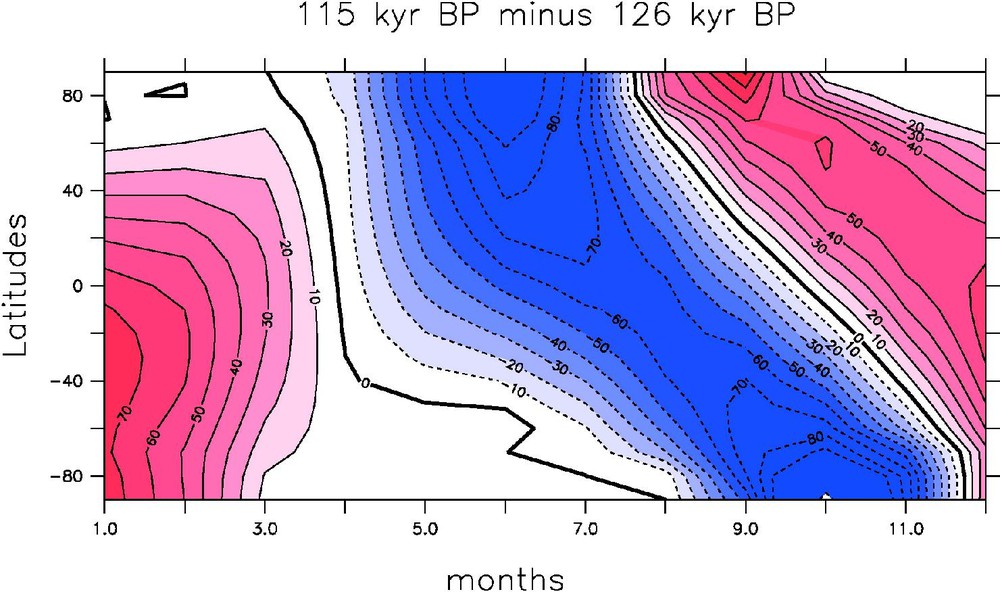
Insolation change at the top of the atmosphere (in Wm-2), differences between 115 kyr BP, corresponding to the inception, and 126 kyr BP, corresponding to the optimum interglacial. Contour intervals are every 10 Wm-2.
Changement d'insolation au sommet de l'atmosphère entre 115 ka, correspondant à la transition interglaciaire/glaciaire, et 126 ka, correspondant à l'optimum interglacière.
During the last decade, with a major increase in palaeoclimatic reconstruction and modelling studies, it appears that these failures were due to two major weaknesses. First, whereas the atmospheric model amplified the cooling due to reduced summer insolation, it was still far to become cold enough to prevent snow from melting. Second, because of the cooling, the wintertime atmosphere was also drier, therefore preventing any increase in snowfall rate. In the 1990s, the idea developed that the sensitivity of the model was too weak, because some important components of the climate system were missing, like the vegetation and the ocean. In a subsequent set of experiments, it has been shown that taking into account the changes in vegetation produced by a colder climate helped to amplify the initial simulated cooling. In response to the atmospheric model cooling, there is a southward progression of areas covered by Tundra (short and scattered type of vegetation) in northern high-latitude lands at the expense of boreal forests [8,15]. This sole change amplified the high-latitude albedo and increased the length of the season of snow-covered lands. Nevertheless, even if the biosphere plays an important role and increases the duration of the snow cover, this feedback remains too weak to lead to perennial snow cover.
2.2 The water cycle and the role of the ocean
Indeed, the second important component, which was missing in these simulations, is the ocean. The first simulations using AGCM assessed that the sea-surface temperatures (SSTs) at the end of Last Interglacial, were very similar to present-day ones, a statement, in the light of recent SSTs reconstruction for this period, that turned out to be false [7]. A first attempt to account for insolation changes on SSTs was performed by Dong and Valdes [9], who coupled the UGAMP AGCM to a slab-ocean model. This study shows that indeed the ocean reacts to changes in insolation, but the response appears to be too large compared to the data [6,7]. Moreover, such a slab ocean is only able to depict the thermal response of the 50-m mixed layer and does not account at all for changes in ocean dynamics. The next step was therefore to use an atmosphere–ocean general circulation model. This step became possible at the beginning of this century, when coupled ocean–atmosphere models were able not only to produce reliable results over continents and oceans, but also when they were able to predict a good sea–ice seasonal cycle, which is a key feature to cope with the inception period. More recently, Meissner et al. [27] showed that only a synergy of ocean atmospheric and vegetation allows producing the onset of ice sheets.
A coupled OAGCM simulation has been performed using IPSL OAGCM and the results can now be directly compared with SSTs inferred from marine cores [22]. The comparison between model results and SSTs reconstructions in the North Atlantic, which is the key region for this study, is shown in Fig. 2. The remarkable feature is that the geographical pattern is very well reproduced: a cooling over the high latitudes of North Atlantic, whereas the tropical North Atlantic is warmer or similar to present-day temperatures. As we will discuss later, this feature is very important to understand the impact of the water cycle on climate. Fig. 3a shows that the summer snow depth increases over regions where it is believed that ice sheets began to grow. After several years, for a grid point corresponding to the Canadian Archipelago, the 115-kyr-BP simulation is able to produce perennial snow cover and then snow accumulation [22] (see Fig. 3b). In this study, it has been shown that superimposed on an increase of about 3% of the northward atmospheric heat transport, there is also a decrease, of about 6%, of the northward ocean heat transport. The location of the deepwater formation is shifted to lower latitudes, due to the increased sea ice extension, whereas the depth of the North Atlantic Deep Water is reduced by about 1000 m.
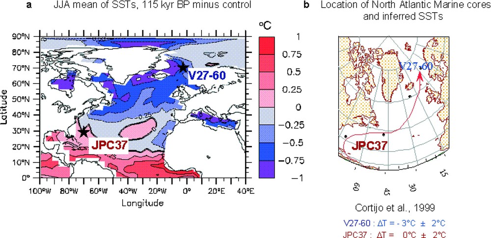
Model-data comparison for SST in the North Atlantic Ocean. (a) Sea-surface temperature (SST) calculated by the IPSL coupled model for the last glacial inception climate (in Celsius) with respect to the simulated present-day climate (control). (b) Location of V27-60 and CH69-K9 marine cores in the North Atlantic Ocean and inferred SST shown with respect to the present-day one. The red arrow traces the main pathway of present-day North Atlantic drift.
Comparaison des résultats de modèles pour les températures de surface de l'Atlantique nord. (a) Température de surface de l'océan (SST) calculée par le modèle OAGCM de l'IPSL entre 115 ka BP et le présent. (b) SST reconstruites à partir des carottes marines de l'Atlantique nord V 27-60 et CH69-K9, entre 115 ka et le présent. Les tirets rouges représentent la dérive nord-atlantique actuelle.
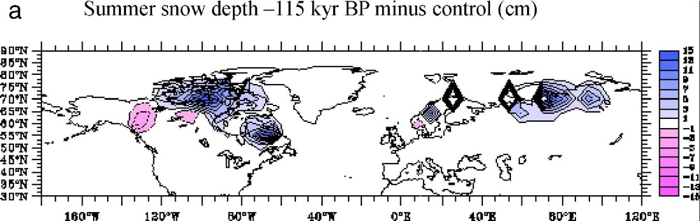
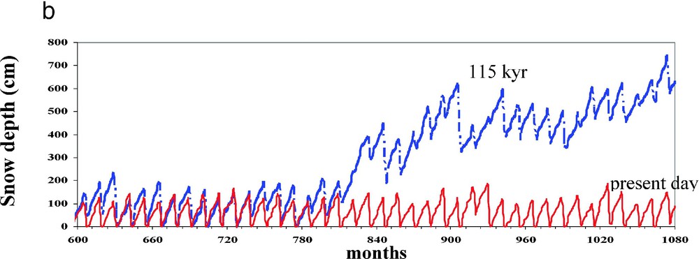
(a) Increased summer snow depth (in cm) over North America and northern Europe simulated by the IPSL model for the last glacial inception with respect to the present-day climate. The values are scaled between ±15 cm with a 2-cm interval. The blue (red) shading indicates an increase (decrease). (b) Snow accumulation over the Canadian Archipelago during the present-day simulation (red curve) and simulation at 115 kyr (blue curve). Each year, the summer snow depth decreases to zero in the control run, whereas, in the simulation at 115 kyr BP, there is clearly a large accumulation of snow and a perennial cover.
(a) Épaisseur de neige estivale (cm) au-dessus de l'Amérique du Nord et de l'Europe, simulée par le modèle de l'IPSL pour l'entrée en glaciation par rapport à l'Actuel. Les valeurs s'étalent entre ±15 cm, avec un intervalle de 2 cm. La couleur bleue indique une augmentation, le rouge une diminution. (b) Accumulation de neige sur l'Archipel canadien pour l'Actuel (en rouge) et pour 115 ka (en bleu). On constate que la neige ne s'accumule pas à l'Actuel et fond totalement en été, tandis qu'on observe, à 115 ka, de la neige pérenne et une forte accumulation.
On the other hand, the amplified North Atlantic SSTs gradient due to the insolation changes induces a larger northward atmospheric moisture transport from the warmer tropical ocean and provides by this way an excess of moisture availability for high latitudes. In this coupled experiment, the simulated water cycle changes have three major impacts over the high latitudes climate:
- (i) the annual mean increase of water runoff into the Arctic Ocean induces an extension and deepening of the halocline, which, associated to cooler surface water, allows a progression of Arctic sea ice volume and extension. This change in sea ice characteristics contributes to enhance the cooling of surrounding lands, like the Canadian Archipelago, because of the increased local albedo;
- (ii) the increase of freshwater input into the Arctic Ocean induces a reduction of the sea surface salinity. The subsequent reduced meridional density gradient in the northern seas leads to a shift of deepwater formation location toward lower latitudes, which, in turn, inhibits the possibility of bringing heat by ocean dynamics toward high latitudes;
- (iii) finally, because of the amplified high latitudes cooling by both feedbacks described herein (points 1 and 2), the increase in water transport towards high latitudes is translated into increased snowfall over regions where ice sheets will grow.
The major advance of this study compared to previous experiments was to show that, before accumulating snow and therefore triggering the ‘Milankovitch’ effect, it is necessary to provide more moisture in northern high latitudes. These changes in the water cycle will amplify the high latitudes cooling due initially to the insolation changes through an intricate network of feedbacks – involving sea ice and ocean –, but will also moist the atmosphere where snow delivery has to increase. All these reasons make the water cycle an important contributor to the shift from interglacial to glacial states all along glacial cycles of the Quaternary.
3 The origin of the Indian Monsoon
The second example illustrating the role of the water cycle in climate change concerns the origin of the Indian monsoon. Many studies [24–26] invoke the fact that, during the Late Tertiary, the uplift of the Tibetan Plateau and Himalaya plays a major role in the development of the Indian monsoon. The main feature of the present-day monsoon is obviously the heavy summer rainfalls over southeastern Asia. These rainfalls are the result of a huge moisture advection driven by the Indian Ocean–Eurasian continent thermal gradient. A change in the Indian Ocean–Eurasia thermal gradient should consequently modify the Asian monsoon. Thus, at geological timescales, plate tectonics should be able to modulate the intensity and location of the Asian monsoon.
Kutzbach et al. [24–26] proposed that the uplift of the Himalaya mountain range as well as of the Tibetan plateau in response to the India–Asia collision has driven the onset of Indian monsoon. The height of the Tibetan plateau and Himalaya appears to be a key forcing factor in the development of the Asian monsoon. They showed, using an AGCM, that the uplift of the Tibetan plateau enhanced the summer monsoon precipitation over southeastern Asia. These experiments were limited by two major aspects:
- – the coarse spatial resolution of the AGCM used in their study does not allow for the representation of the Himalaya mountain ranges; the Himalayan and the Tibetan plateau are represented by a single geological structure;
- – their study consisted in three crude sensitivity experiments to the height of the Tibetan plateau. In a first step, the whole plateau is lowered to 400 m (no plateau experiment), then the present-day elevation of the Tibetan plateau is reduced by a half (half-elevation experiment), and at last, they simulate the climate using the present day topography (full elevation experiment).
Although the AGCM was forced using a crude palaeogeography, they clearly show that the intensity of the Asian summer monsoon is a function of the elevation of the Tibetan plateau.
The palaeogeographical context evolved drastically over the past 30 Myr in Eurasia (Fig. 4). The major striking features are:
- (i) the rise of the Tibetan plateau and of the Himalayas chain. Although the India-Asia collision is at the origin of these uplifts, the evolution of these two geological objects is different;
- (ii) the lateral extrusion of Indochina as a consequence of the India-Asia collision;
- (iii) the progressive shrinkage of the Paratethys Sea, which covers the eastern part of Europe and a large part of Siberia and Central Asia, in response to the large-scale deformation of the southern margin of Eurasia.
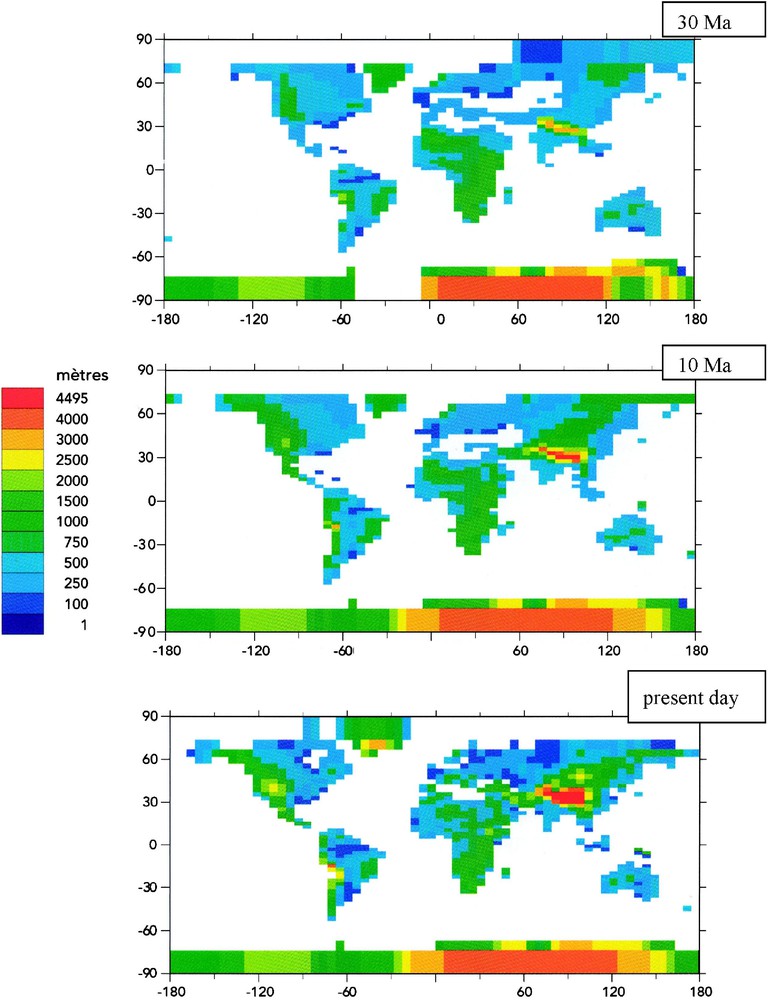
Palaeogeography at 30 Myr (top), at 10 Myr (middle) and at the present day (bottom) used as boundary conditions [3,4]. The main changes are the uplifts of the Himalayas and of the Tibetan plateau, and the progressive retreat of an epicontinental sea in Eurasia, the Paratethys Sea. The Middle East emerged during the Early Miocene, as well as the lateral extrusion of Indochina, in response to the India–Eurasia convergence. White areas represent oceans and seas.
Paléogéographies à 30 Ma (haut), 10 Ma (milieu) et actuelle (bas), utilisées comme conditions aux limites des simulations avec LMDZ. Les principaux changements sont la surrection du plateau tibétain et de la chaîne Himalayenne, ainsi que le retrait progressif de la mer épicontinentale Paratéthys. Le Moyen Orient émerge dès le début du Miocène, ainsi que l'extrusion latérale de l'Indochine liée à la convergence Inde–Asie.
We used the LMD AGCM numerical model to simulate the climate corresponding to these two different periods: 30 Myr ago, a situation where the Paratethys is large and for which there is no uplift; and 10 Myr ago, a situation where the Paratethys has already shrunk, while the plateau uplift is already important.
In a first step, we performed experiments with the most realistic palaeogeography for 30 and 10 Myr [14,29]. Forcing the AGCM with a set of boundary conditions representing the major features of the Oligocene period, we showed that a monsoon circulation producing rainfall mainly over Indochina existed prior to the main uplift of the Tibetan Plateau and the Himalaya (Fig. 5).
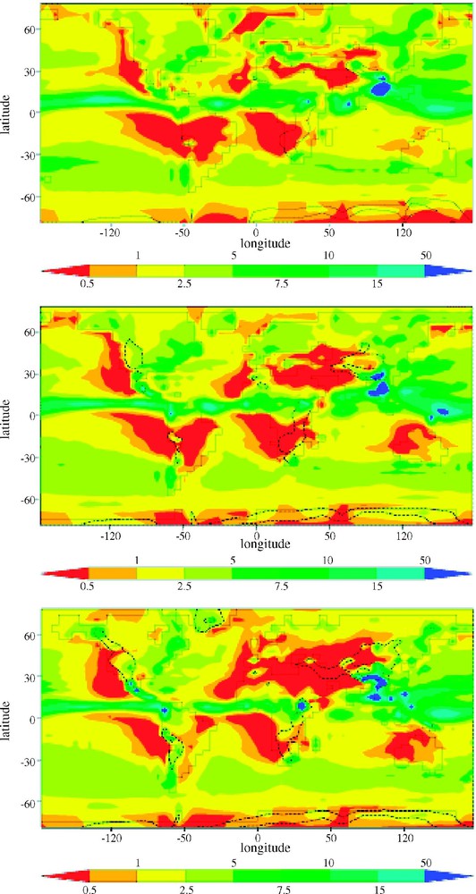
Simulated summer precipitation (mm d−1) at 30 Ma (top), at 10 Ma (middle) and at PD (bottom).
Précipitations d'été simulées (mm j−1) à 30 Ma (haut), à 10 Ma (milieu) et à l'Actuel (bas).
The change in palaeogeography enhanced the summer thermal gradient, increasing the moisture advection over southern Asia, inducing heavy rainfalls during the summer. However, the change in monsoon is not only due to a change in the thermal gradient. The atmospheric circulation is also deeply altered. The intensity and direction of winds are changed, bringing more and more moisture towards the Himalaya chain in the two last experiments, at 10 Myr and nowadays. The rise of moist air masses along the Himalayan southern flank generates heavy rainfalls over this mountain range (Fig. 5), enhancing the mechanical erosion of the Himalaya [14,26].
The thermal evolution of the Asian continent from a seasonal point of view clearly appears to be a key characteristic for the monsoon evolution. In Fig. 6, we show the winter and summer air temperature differences between 30 and 10 Myr. As we could expect, the shrinkage of the Paratethys (i.e. the fact that an epicontinental sea disappears) has for consequences the warming of the Eurasian continent during the summer season and its cooling during the winter season (Fig. 6).
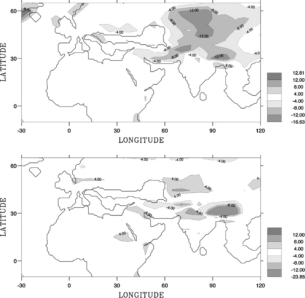
Temperature difference (°C) in winter (top) and summer (bottom) between the experiment at 10 Myr and that at 30 Myr. Dashed (continuous) lines represent isotherms below (above) 0 °C.
Différence de température d'hiver (haut) et d'été (bas) entre les simulations à 10 et 30 Ma. Les lignes pointillées (continues) représentent les isothermes au-dessous (au-dessus) de zéro.
Moreover, it is possible with a GCM to quantify the separate impact of the uplift of the Tibetan Plateau and Himalayas and that of the shrinkage of the Paratethys. We therefore performed two more experiments: one without uplift and a second without shrinkage.
In fact, these simulations [14,29] showed that the plate tectonics modulates the distribution and intensity of the Asian monsoon at the geological time scale, but that the monsoon over southeastern India did exist already during the Oligocene or Early Miocene [5,13,20]. Both the uplift and the shrinkage act on the summer thermal gradient between Asia and the Indian Ocean, and modify the atmospheric circulation and moisture advection to modulate the summer geographical pattern of monsoon.
As shown in Fig. 7, the difference on rainfall due to the plateau uplift is nevertheless much more local (linked to the orogenesis), whereas the shrinkage of the epicontinental sea has a broader and more regional effect. The redistribution of monsoon rainfall is largely driven by palaeogeographic evolution at this timescale.
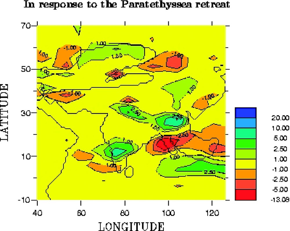
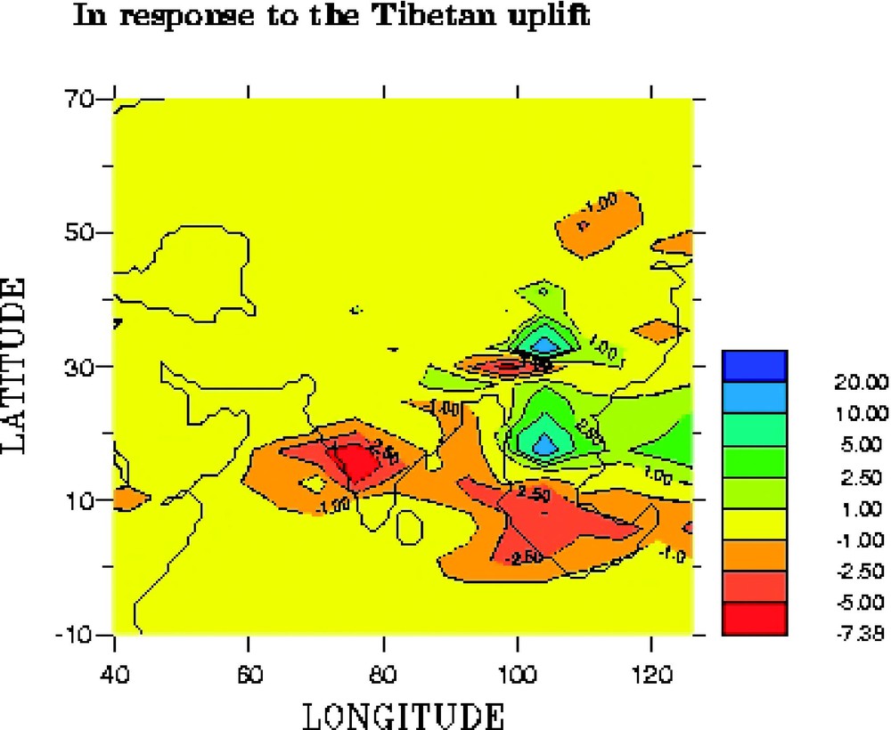
Sensitivity experiments to the Tibetan Plateau and Himalayas' uplifts (top) and to the Paratethys shrinkage (bottom). The impact of the uplift on summer precipitation is more local than the impact of the Paratethys shrinkage.
Expériences de sensibilité à la surrection du plateau tibétain et de la chaîne himalayenne (haut) et au retrait de la Paratéthys (bas). L'impact de la surrection sur les précipitations est plus local que celui du retrait de la Paratéthys.
4 Glaciations of the Neoproterozoic
4.1 Snowball hypothesis
The Earth's history is surprising. Due to a fainter sun (the insolation at the top of the Earth's Atmosphere has increased from 80% to the present-day value during the last 2 Gyr), the surface of the Earth should have been covered with ice. Such a result has been simulated with a simple Energy Balance Model [2].
But to get out of a snow-covered Earth, the so-called ‘snowball Earth’, an enormous quantity of energy is necessary due to the obviously very large albedo. Indeed, the albedo of a snowball Earth is around 0.7, whereas the present-day albedo is around 0.3. Therefore, in a snowball Earth context, most of the incoming solar radiation is reflected. This feature explains the difficulty to initiate deglaciation from an Earth totally covered with ice. This paradigm lasted for more than 20 years, until Kirschvink [24] argued that a very important component was missing in the Budyko scenario (only accounting for albedo changes in an EBM model): the carbon cycle.
Indeed, if the Earth were totally covered with ice sheets over continents and sea-ice over oceans, the water cycle would be seriously damped by a factor form 10 to 100, depending on the simulations [4,12]. Most importantly, the sink of carbon at geological timescales (the continental weathering) shuts off, while the source of carbon (the outgassing through volcanoes and the mid-oceanic ridge) keeps on injecting CO2 in the atmosphere, where it accumulates for millions of years. When the atmospheric CO2 content reaches a threshold value estimated to be 0.12 bar [3], a huge deglaciation occurs and produces the so-called cap-carbonates seen everywhere above the Neoproterozoic glacial sediments. Such a scenario may also explain the reappearance of the banded iron formations (BIF), which have disappeared since 2.4 Gyr and were due to global anoxia in the ocean.
These scenarios led a lot of climate modellers to quantitatively test these ideas of a large or full glaciation during the Neoproterozoic. Many GCM models and simulations with more simple models [11,21] show that it was possible to simulate a snowball Earth in the Neoproterozoic context (i.e., accounting for palaeogeography, weaker insolation by 6%, and rather low value of CO2). The results of the IPSL LMDz OAGCM coupled with a swamp model for Sturtian palaeogeography are presented.
The fact that the reduction of the solar constant is large enough to produce a global glaciation in our numerical simulations is in reality facilitated by the low atmospheric CO2 level, which cannot compensate for the deficit of solar energy due to the faint young Sun.
4.2 Carbon cycle
Most of the obtained results strongly depend on the prescribed atmospheric CO2 level in these simulations. There is indeed no way to infer from any proxy the value of atmospheric CO2 during these extreme events. The only way to assess a consistent value between climate and carbon cycle is to use a carbon–climate model adapted for geological timescales. To achieve this goal, the model of intermediate complexity, CLIMBER-2, [16,17], has been coupled to the COMBINE model, which calculates the main features of C, P, and O biogeochemical cycles [19].
The most difficult challenge is to explain why the CO2 should have strongly decreased and therefore triggered the onset of a global glaciation. Using our new model, called GEOCLIM (for GEOlogical timescales CLImate Model), we have shown that tectonics plays a major role during the Neoproterozoic [10,30]. The dispersal of the Rodinia supercontinent results in an enhanced consumption of atmospheric CO2, decreasing from a pCO2 of 1830 ppm to 510 ppm, i.e. consumption in the order of 1320 ppm. This is due to the larger runoff occurring over the equatorial regions presenting a dispersed configuration, which triggers larger weathering rates, and a significant global cooling of (Fig. 8). We have further demonstrated that experiments accounting for the palaeogeographic impact on weathering rates together with the weathering of the large magmatic provinces produce conditions appropriate to trigger a full snowball glaciation at 750 Ma (Fig. 9). Indeed, the break-up of the Rodinia supercontinent is heralded by and accompanied with the eruptions of large basaltic provinces [27], resulting in an increase of the weatherability of the continental surface and consumption of atmospheric CO2 over the long timescale [18].
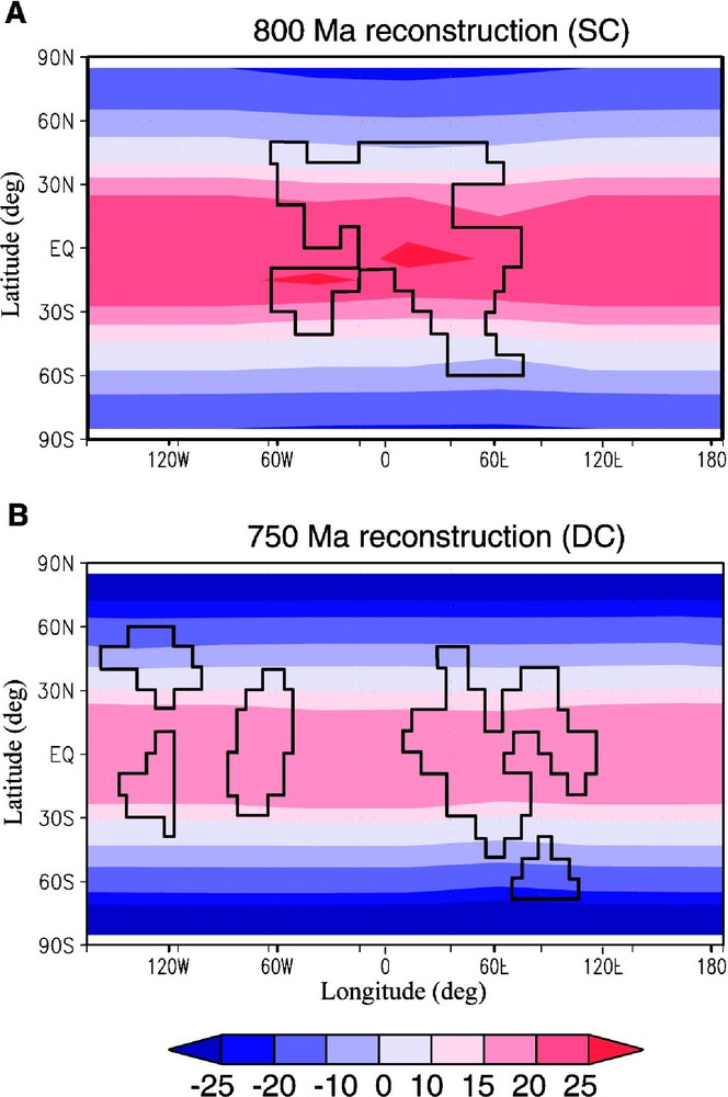
Annual mean surface air temperature (°C) simulated by the CLIMBER-2 model. (A) With a pCO2 of 1830 ppm and for the continental reconstruction at around 800 Myr [30,31] (noted SC as Supercontinent Configuration), i.e. prior to the Rodinia break-up. (B) With a pCO2 of 510 ppm and for the continental reconstruction at around 750 Myr [32] (noted DC as Dispersed Configuration). Boundary conditions include a solar luminosity 6% below the present-day value. In addition, we assume that the Earth's orbit around the Sun was circular (eccentricity = 0) and that the Earth's obliquity was 23.5°. This setting leads to an equal annual insolation for both hemispheres. The land surface in the climate model has the radiative characteristics of a desert and has a uniform elevation of 100 m for both palaeogeographies.
Moyenne annuelle des températures de surface simulées par le modèle CLIMBER-2. (A) avec pCO2 = 1830 ppm, et reconstruction continentale correspondant à 800 Ma [30,31] (notée SC, supercontinents antérieurs au break-up) ; (B) avec pCO2 = 510 ppm, avec une configuration des continents correspondant à 750 Ma [32] (noté DC, continents dispersés). Les deux expériences sont effectuées avec une baisse de l'insolation au sommet de l'atmosphère de 6%, par rapport à la valeur actuelle. L'excentricité de l'orbite est nulle et l'obliquité de 23,5°. Le relief a une élévation de 100 m, pour les deux paléogéographies.
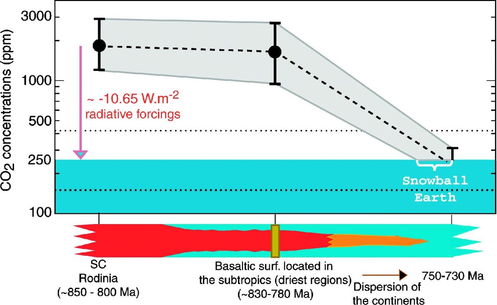
Steady-state atmospheric CO2 level achieved by GEOCLIM (1) for the SC runs, (2) for the SC runs with the inclusion of basaltic provinces, and (3) for the DC runs also with basaltic provinces. Vertical bars denote the upper and the lower range of atmospheric CO2 levels, calculated using (1) a 20% increase and a 20% decrease in degassing flux for the SC runs, (2–3) a 20% increase and a basaltic surface of , and a 20% decrease and a basaltic surface of for the SCtrap and DCtrap runs.
Niveau à l'équilibre de CO2 atmosphérique calculé par GEOCLIM (1) pour la simulation « SC », (2) pour la simulation « SC trap » incluant les basaltes, (3) pour la simulation « DC trap » incluant également les basaltes. L'enveloppe représente les niveaux de CO2 atmosphérique maximum et minimum calculés par le modèle (1) pour des valeurs du dégazage augmentées et/ou diminuées de 20% par rapport à sa valeur actuelle (2–3) pour une valeur du dégazage augmentée de 20% et une surface basaltique de et pour une valeur de dégazage diminuée de 20% et une surface basaltique de , et ce pour les runs « SC trap » et « DC trap ».
These studies provide support for the fact that the modification of the water cycle in response to the shift of continental plates may have been responsible for a long-term atmospheric CO2 decrease. The efficiency of the proposed mechanism relies on the tropical position of the continents at this time. Indeed, the water cycle is very efficient over this region. The increase in runoff is able to produce a huge consumption of atmospheric CO2 via the continental weathering processes.
5 Conclusion
These three very different contexts illustrate the role of the water cycle in Earth's Climate history at various timescales. From clouds to sea ice and from ice sheets build-up to thermohaline circulation, water is one of the key components of the Earth System. Many processes are very short (clouds physics), but others explain climate changes at Myr scales (weathering and CO2 burial).
What has been shown for the Earth's history is also true for the future climate of our planet.
The climate of the beginning of this century should be dominated by the impact of greenhouse gases (and water is one of these gases). With increasing temperature, the capability of atmosphere to contain water vapour will also increase and this is a positive feedback, which in turn will lead to increase again the temperature. This scenario has to be modulated because of cloud changes that may have positive (high clouds) or negative (low clouds) feedbacks.
Obviously, the sea level will rise with the glaciers disappearance, but, more importantly, the problem may come from the destabilisation of the ice sheets (Greenland and Antarctica). How fast may this occur? Which meltwater amount does it induce? How may Global Climate and thermohaline circulation be affected? Models that have been tested on past climate changes may be helpful to try to give a quantified answer to these questions.