Steady-state vertical distribution of cohesive sediments in a flow

Martin Sánchez; Patricia Grimigni; Yann Delanoë

doi:10.1016/j.crte.2004.10.020

Résumés

Anglais
Français

Settling velocity of diluted suspended aggregates is examined under steady-state conditions. It is shown that if the local settling velocity of the suspended mass of sediments at the bottom is gamma distributed, then, the vertical variation of the local mean settling velocity $\bar{W}$ is proportional to a power $1 / r$ of the local concentration C, where r is the gamma distribution parameter. That is a consequence of the suspended-sediment sorting produced by the vertical dynamics. The parameter r characterizes the range of settling velocity values for all the aggregates simultaneously in suspension.

La vitesse de chute des matières en suspension peu concentrées est étudiée en régime stationnaire. On montre que, si la vitesse de chute de la masse des sédiments en suspension au fond est distribuée selon une loi gamma de paramètre r, alors la variation verticale de la vitesse de chute moyenne locale $\bar{W}$ est proportionnelle à une puissance $1 / r$ de la concentration locale C. Ceci s'explique par une ségrégation des matières en suspension provoquée par la dynamique verticale sédimentaire. Le paramètre r caractérise l'étendue des valeurs de la vitesse de chute pour l'ensemble d'agrégats simultanément en suspension.

Version française abrégée

1 Introduction

La vitesse de chute de sédiments cohésifs en suspension dans les cours d'eau est très supérieure à celle des grains d'argile individuels. Ceci s'explique par le fait que la plus grande partie de la masse sédimentaire en suspension se rassemble sous la forme d'agrégats [9]. La vitesse de chute synthétise certaines caractéristiques de ces agrégats, telles que la taille, la forme et la masse volumique.

La vitesse de chute intervient dans deux phénomènes sédimentaires de première importance, qui sont la répartition verticale des matières en suspension (MES) et leur flux de dépôt. La vitesse de chute varie principalement en fonction de la concentration locale C [4,5,11]. Pour les suspensions diluées, la vitesse de chute augmente avec C. Pour les suspensions très concentrées $(C > \sim 10 kg m^{−3})$ , la vitesse de chute diminue quand C augmente (vitesse entravée). Cette étude porte essentiellement sur la vitesse de chute de suspensions diluées.

La plupart des auteurs caractérisent la vitesse de chute par sa valeur médiane locale $W_{50 %}$ , qui est toujours inférieure à la vitesse de chute moyenne locale $\bar{W}$ , laquelle donne une meilleure description de la dynamique verticale des sédiments. Dans les modèles hydrosédimentaires, la vitesse de chute est usuellement représentée par un scalaire dont la valeur dépend de C [3–5,7,10,11] ; cependant, compte tenu du grand nombre d'agrégats divers se trouvant simultanément en suspension, la vitesse de chute est en réalité une variable stochastique. Une variable aléatoire W est définie comme la vitesse de chute d'un élément constitutif des MES de masse unitaire infinitésimale.

2 Théorie

Une distribution verticale stationnaire des MES dans un écoulement est théoriquement possible si, à chaque niveau z, le flux solide vertical descendant lié à $\bar{W}$ est en équilibre avec le flux solide ascendant lié à la diffusion turbulente de masse. Si l'on admet que la diffusion peut être décrite par la loi de Fick, la dynamique verticale des MES peut être modélisée par (1), où z est la coordonnée verticale (positive vers le haut), et $K_{z}$ est le coefficient de diffusion verticale turbulente de masse.

Ainsi, si $\bar{W}$ est constant sur z, la répartition verticale de C est régie par une loi généralisée de Rouse–Vanoni (2) [5], où $C_{a}$ est une valeur de référence de C près du fond (mesurée à une distance du fond $z = a$ ).

La dynamique verticale des MES provoque une ségrégation des agrégats, de sorte que les vitesses de chute des sédiments du fond sont plus élevées que celles des sédiments superficiels [2]. Comme la concentration décroît aussi avec z, la variation verticale de $\bar{W}$ avec C peut être modélisée par la loi de puissance (3), où $\bar{W_{a}}$ est la vitesse de chute moyenne des sédiments près du fond, et r est un paramètre. Dans ce cas, la répartition verticale des MES n'est plus donnée par (2), mais par (4), avec $λ_{z} = r / \bar{W}$ donné par (5), où $λ_{a} = r / \bar{W_{a}}$ .

Le profil vertical de C dépend de l'expression retenue pour décrire $K_{z}$ . Par exemple, pour $K_{z}$ constant sur la verticale, si la concentration de référence au fond est mesurée en $z = a = 0$ , alors $λ_{z} = λ_{a} + z / K_{z}$ . Si, pour chaque niveau z, la fonction de densité de probabilité (fdp) $f_{W} (w)$ de la variable aléatoire W est en accord avec la loi de distribution gamma définie par (6), alors, pour chaque valeur w de W, la distribution verticale des matières en suspension est compatible avec la loi généralisée de Rouse–Vanoni, et avec les Éqs. (3), (4) et (5) [1].

De plus, le paramètre r intervenant en (3) et (6) et caractérisant l'étendue de valeurs de W satisfait à l'Éq. (7) [8], où $σ [W]$ est l'écart type des valeurs locales de W et $σ [W_{a}]$ est celui de W au fond. Si les interactions entre agrégats peuvent être négligées quand $C_{a}$ demeure constant dans le temps, le paramètre r peut être considéré comme un caractère intrinsèque des MES pour chaque valeur de $C_{a}$ .

Si une vitesse de chute locale adimensionnelle est définie par $W^{*} = W / \bar{W}$ , alors la fdp de $W^{*}$ pour chaque niveau z est en accord avec la loi de distribution gamma standardisée définie par (8).

En régime stationnaire, on peut montrer que si, pour un sédiment donné, la fdp de W au fond est décrite par une loi gamma, alors la variable aléatoire W, à n'importe quel niveau z, est aussi distribuée selon une loi gamma de même paramètre r [1]. Dans ce cas, la variation verticale de $\bar{W}$ en fonction de C est régie par (3), indépendamment de l'expression retenue pour décrire $K_{z}$ . La validité de l'Éq. (3) peut être étendue pour une distribution verticale des matières en suspension variant graduellement en fonction du temps, à condition que la concentration C décroisse d'une façon monotone du fond de la colonne d'eau vers la surface.

Tous ces résultats sont compatibles avec les expressions usuelles de $K_{z}$ , lesquelles peuvent éventuellement tenir compte de l'effet d'une stratification verticale de la masse volumique de l'eau [5]. La forme la plus connue du modèle de Rouse–Vanoni pour la distribution verticale des matières en suspension est obtenue en prenant $K_{z} = κ U^{*} z (1 - z / d)$ , où κ est la constante de Karman, $U^{*}$ la vitesse de cisaillement, et d la profondeur totale.

Le Tableau 1 donne, pour plusieurs valeurs de r, les valeurs de $σ [W] / \bar{W}$ , de $\bar{W} / W_{50 %}$ , et de $W_{90 %} / W_{10 %}$ (où $W_{N %}$ représente la valeur de W ayant N% de probabilité de ne pas être dépassée par la masse sédimentaire). La Fig. 1 montre la fonction de répartition $F (w^{*})$ associée à (8) en termes de $w^{*}$ , qui est représenté à l'échelle logarithmique. La fonction de répartition $F (w^{*})$ représente la proportion en poids des matières en suspension avec des valeurs de $W^{*}$ inférieures à $w^{*}$ .

r	$σ [W] / \bar{W}$	$\bar{W} / W_{50 %}$	$W_{90 %} / W_{10 %}$
0.25	2.0000	5.7243	11116
0.50	1.4142	2.1981	171.3
1.00	1.0000	1.4427	21.85
2.00	0.7071	1.1966	7.31
4.00	0.5000	1.0893	3.83
∞	0.0000	1.0000	1.00

Fig. 1
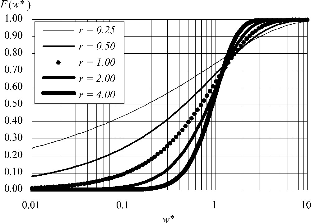
Cumulative distribution function linked to the pdf $f_{W^{*}} (w^{*})$ of $W^{*}$ (Eq. (8)), for five values of the parameter r.
Fonction de répartition associée à la fonction de densité de probabilité $f_{W^{*}} (w^{*})$ de $W^{*}$ (Éq. (8)), pour cinq valeurs du paramètre r.

À titre d'exemple, la Fig. 2 montre, pour $r = 2$ et un nombre de Péclet $Pe = \bar{W_{a}} d / K_{z} = 2$ , avec $K_{z}$ constant sur la verticale, quelques aspects de la distribution verticale des MES. La Fig. 2a représente la répartition verticale de $C / C_{a}$ . La Fig. 2b montre, pour cinq valeurs de $z ° = z / d$ , la distribution locale des MES $SC (w °)$ rapportée à la concentration au fond $C_{a}$ en termes des valeurs possibles w° de la variable aléatoire $W ° = W / \bar{W_{a}}$ décrivant une vitesse de chute non locale adimensionnelle. Le produit $SC (w °) d w °$ représente la quantité de masse par unité de volume ayant des valeurs de W° comprises entre $w ° - d w ° / 2$ et $w ° + d w ° / 2$ . Enfin, la Fig. 2c montre la variation verticale de $SC (w °)$ rapporté à la distribution au fond des MES ${SC}_{a} (w °)$ , pour quatre valeurs de w°. Pour chaque valeur w° de W°, la distribution locale des MES est régie par la loi exponentielle en z, $SC (w °) = {SC}_{a} (w °) \exp (- Pe w ° z °)$ . Une autre propriété de la fdp gamma définie par (6) est que, quand l'Éq. (5) est complétée par (9), le rapport $SC (w °) / {SC}_{a} (w °)$ est décrit par la forme la plus connue du modèle de Rouse–Vanoni, et ceci d'une façon exacte pour chaque valeur w° de W°.

Fig. 2
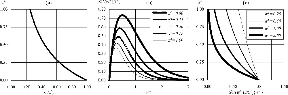
Suspended sediment vertical distribution for $K_{z}$ depth-invariant, r=2, and a Péclet number $Pe = \bar{W_{a}} d / K_{z} = 2$ . (a) Vertical variation of the ratio $C / C_{a}$ . (b) Variation of $SC (w °) / C_{a}$ in terms of w°, for five values of z°. (c) Vertical variation of $SC (w °) / {SC}_{a} (w °)$ , for four values w° of W°.
Répartition verticale des matières en suspension pour r=2 et un nombre de Péclet $Pe = \bar{W_{a}} d / K_{z} = 2$ , avec $K_{z}$ constant sur la verticale. (a) Variation verticale du rapport $C / C_{a}$ . (b) Variation de $SC (w °) / C_{a}$ en termes de w°, pour cinq valeurs de z°. (c) Variation verticale de $SC (w °) / {SC}_{a} (w °)$ , pour quatre valeurs w° de W°.

3 Méthodes et résultats

Dans le but d'étudier la répartition verticale des MES et leurs vitesses de chute, six tests ont été effectués sur des échantillons prélevés dans l'estuaire de la Loire simultanément au fond, à mi-profondeur et en surface [1] (Tableau 1). La distribution locale des MES en termes de vitesses de chute a été examinée par la méthode du tube de décantation [6].

La Fig. 3 montre les fréquences cumulées expérimentales de $W^{*} = W / \bar{W}$ en termes de ses valeurs possibles $w^{*}$ (avec $\bar{W}$ calculé par (3) et (10)). Les deux répartitions suivantes n'ont pas été représentées : celle du test n°1 à mi-profondeur (erreur expérimentale) et celle du test n° 5 au fond (concentration excessive, incompatible avec la méthode du tube de décantation). La Fig. 3 montre aussi la fonction de répartition $F (w^{*})$ résultant de l'intégration de le fdp définie par (8), avec r calculé par (11), c'est-à-dire sans ajustement spécifique à chaque test. La vitesse de chute moyenne des sédiments du fond $\bar{W_{a}}$ (m s⁻¹) et le paramètre r sont rattachés à $C_{a}$ (kg m⁻³) par les lois (10) et (11), propres à la vase de Loire.

Fig. 3
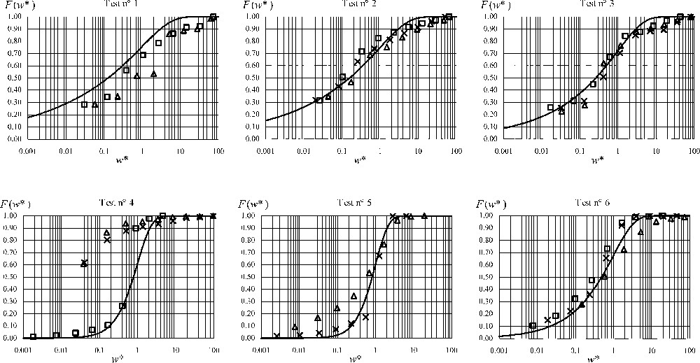
Experimental cumulative frequencies of $W^{*} = W / \bar{W}$ , with $\bar{W}$ calculated using Eqs. (3) and (10) (× = surface – ▴ = half-depth – □ = bottom), and in continuous line, the cumulative distribution function $F (w^{*})$ associated with the pdf defined by Eq. (8) with the parameters r evaluated with Eq. (11).
Fréquences cumulées expérimentales de $W^{*} = W / \bar{W}$ , avec $\bar{W}$ calculé par (3) et (10) (× = surface – ▴ = mi-profondeur – □ = fond), et en courbe continue, fonction de répartition $F (w^{*})$ résultant de l'intégration de le fdp définie par (8), avec r calculé par (11).

Ces lois sont confirmées par huit autres mesures in situ avec un tube d'Owen $(0, 25 kg m^{−3} < C_{a} < 3 kg m^{−3})$ , et par des mesures en laboratoire sur des échantillons reconstitués dans une gamme de concentrations $10 kg m^{−3} < C_{a} < 15 kg m^{−3}$ , dans laquelle la vitesse de chute moyenne reste à peu près constante avant que la vitesse entravée ne soit observée [1,7].

D'une façon générale, pour $F (w^{*}) > 0, 1$ , la fdp standardisée définie par (8) s'accorde bien avec les valeurs expérimentales de la distribution statistique de $W^{*}$ . Les seules exceptions à cette règle sont les résultats obtenus lors du test n° 4 sur les échantillons de mi-profondeur et de surface. Ces exceptions pourraient s'expliquer par la présence au fond, le jour du prélèvement, d'une lentille de crème de vase ayant pu provoquer, par suite d'une contamination de l'échantillon, une surestimation de la concentration de référence au fond. Ce bon accord justifie ici l'utilisation de l'Éq. (3), dont la validité est, dans ce cas, analytiquement démontrée pour un régime stationnaire [1]. La distribution verticale des matières en suspension dans l'estuaire de la Loire peut ainsi être considérée comme étant graduellement variée dans le temps.

On doit noter que, quand une couche de crème de vase recouvre le fond, la concentration de référence $C_{a}$ doit être mesurée au-dessus de cette couche. En fait, le modèle de Rouse–Vanoni dans l'estuaire de la Loire ne peut être appliqué que si $C_{a} < \sim 15 kg m^{−3}$ . Au-dessus de cette concentration, la vitesse de chute est entravée et les agrégats de vase ne sont pas libres de se déplacer individuellement. En présence d'une couche de crème de vase, la dynamique verticale près du fond serait mieux décrite par un système bicouche que par l'Éq. (1). Dans le test n° 5, la concentration de référence près du fond $C_{a}$ a été prise égale à 15 kg m⁻³.

4 Conclusions

En régime stationnaire, si la vitesse de chute des sédiments du fond est distribuée en accord avec la loi gamma, alors la variation verticale de la vitesse de chute moyenne locale $\bar{W}$ avec la concentration locale C est régie par l'Éq. (3), indépendamment de l'expression retenue pour décrire $K_{z}$ . Ceci est une conséquence de la ségrégation des agrégats, provoquée par la dynamique verticale des matières en suspension.

Ainsi, quand la vitesse de chute de la masse de sédiments en suspension près du fond est distribuée selon une loi gamma, la vitesse de chute moyenne $\bar{W}$ et le paramètre r de la distribution sont suffisants pour décrire la dynamique verticale de toute la population d'agrégats en suspension. Dans ce cas, d'une part, la vitesse de chute moyenne des sédiments du fond doit être rattachée à la concentration $C_{a}$ près du fond $(\bar{W_{a}} = ϕ (C_{a})$ , résultant d'un effet direct de la concentration par floculation) ; d'autre part, la variation verticale de la vitesse de chute moyenne locale peut être décrite par l'Éq. (3) ( $\bar{W} = \bar{W_{a}} {(C / C_{a})}^{1 / r}$ , résultant d'une ségrégation des agrégats provoquée par la dynamique verticale des MES). Cette approche s'avère valable pour les vases de l'estuaire de la Loire, pour des valeurs de $C_{a}$ inférieures à 15 kg m⁻³, ce qui permet de couvrir pratiquement toute la gamme de concentrations qu'on y observe. Finalement, on peut noter que les développements théoriques présentés dans cet article peuvent s'appliquer à la modélisation de la dynamique verticale des sédiments non cohésifs en suspension dans les cours d'eau.

1 Introduction

The settling velocity of cohesive suspended sediments in the natural open surface flows is much higher than that of the elementary clay grains. This is due to the fact that the greatest part of the mass of sediments consists of aggregates, whose weight is largely higher than that of the individual grains [9]. The settling velocity includes a certain number of the characteristics of these aggregates, such as their size, shape and density.

The dynamics of the cohesive sediment is strongly dependent on the settling velocity of the suspended matter. This parameter intervenes in two sedimentary processes of first importance: the vertical distribution of the suspended matter and its deposition rate.

Settling velocity varies mainly with the local suspended sediment concentration C. A great number of field and laboratory measurements [4,5,11] showed that for diluted suspensions, settling velocity increases regularly with the concentration. On the other hand, for the highly concentrated suspensions starting from a concentration of about 10 kg m⁻³, this velocity decreases when the concentration increases because the sediments are blocked in their fall (hindered velocity). What follows deals with the study of the settling velocity of diluted suspensions for concentrations lower than about 10 kg m⁻³.

Most of the researchers characterize settling velocity by its median value. In all the cases, the median settling velocity $W_{50 %}$ is inferior to the mean settling velocity, which multiplied by the concentration gives the downward vertical solid flux, linked to gravity. The local mean settling velocity $\bar{W}$ gives the best description of the downward vertical dynamics of the cohesive sediments.

Settling velocity in sedimentary models is usually represented by a scalar whose value depends mainly on the local suspended sediment concentration [3–5,7,10,11]. However, taking into account the great diversity of aggregates that one can simultaneously find in suspension, the settling velocity is actually a stochastic variable. A random variable W is defined as the settling velocity of a particle of the suspended aggregates of infinitesimal elementary mass.

2 Theory

A steady-state vertical distribution of the suspended sediment in a flow is theoretically possible if at each level z the vertical downwards mass flux due to the local mean settling velocity $\bar{W}$ is equal to the ascending mass flux linked to the turbulent diffusion of sediment. The vertical movement of fine sediments can be expressed by assuming a Fickian mass diffusion as:

\bar{W} C = - K_{z} \frac{\partial C}{\partial z}

(1)

where z is the vertical co-ordinate (positive upwards), and

K_{z}

is the vertical eddy diffusivity coefficient. Then, if

\bar{W}

is depth-invariant, the vertical distribution of the concentration is given by the generalized Rouse–Vanoni law [5]:

C = C_{a} \exp (- \bar{W} \int_{a}^{z} \frac{d z}{K_{z}})

(2)

where

C_{a}

is a reference value of C near the bottom (at height above the bed

z = a

). Actually the suspended sediment vertical dynamics sorts the aggregates so that the settling velocities of the bottom sediments are superior to those of the surface sediments [2]. As C decreases also when z increases, the vertical variation of

\bar{W}

with C can be modelled by the following power law:

\bar{W} = \bar{W_{a}} {(\frac{C}{C_{a}})}^{1 / r}

(3)

where

\bar{W_{a}}

is the mean settling velocity of the near-bottom sediments, and r is a parameter. In this last case, the vertical distribution of the concentration is given by [1]:

C = C_{a} {(\frac{λ_{a}}{λ_{z}})}^{r}

(4)

where

λ_{a} = r / \bar{W_{a}}

, and

λ_{z} = r / \bar{W}

, which is given by:

λ_{z} = λ_{a} + \int_{a}^{z} \frac{d z}{K_{z}}

(5)

The vertical profile of the concentration depends on the expression used to describe $K_{z}$ . For instance, when $K_{z}$ is depth-invariant, if the bottom concentration is taken at $z = a = 0$ , then $λ_{z} = λ_{a} + z / K_{z}$ . If the probability density function (pdf) $f_{W} (w)$ of W for every level z is in accordance with the following gamma distribution:

f_{W} (w) = \frac{λ_{z}^{r} w^{r - 1} \exp (- λ_{z} w)}{Γ (r)} 0 ⩽ w < \infty

(6)

where Γ is a gamma function, then, for every value w of W, the vertical distribution of the suspended matter is compatible with the generalized Rouse–Vanoni law and with Eqs. (3)–(5) [1]. The shape parameter r of the distribution depends on the relative extent of the values of the settling velocity and satisfies to [8]:

r = \frac{{\bar{W}}^{2}}{σ {[W]}^{2}} = \frac{{\bar{W_{a}}}^{2}}{σ {[W_{a}]}^{2}}

(7)

where

σ [W]

is the standard deviation of the local values of W and

σ [W_{a}]

is that of W near the bottom. If the interactions between aggregates are neglected when the near-bottom concentration is time-invariant, the parameter r can be considered as an intrinsic character of suspended aggregates for a given near-bottom concentration.

If a non-dimensional local settling velocity $W^{*}$ is defined in terms of the local mean settling velocity $\bar{W}$ by $W^{*} = W / \bar{W}$ , then, the pdf of $W^{*}$ for every level z is in accordance with the following standardized gamma distribution:

f_{W^{*}} (w^{*}) = \frac{r^{r} {(w^{*})}^{r - 1} \exp (- r w^{*})}{Γ (r)} 0 ⩽ w^{*} < \infty

(8)

In steady-state conditions, if, for a given sediment, the pdf of W linked to the bottom sediments is described by a gamma distribution, then, for every level z, W is also gamma distributed with the same parameter r [1]. In this case, the vertical variation of the local mean settling velocity $\bar{W}$ with the local concentration is governed by the power law defined by Eq. (3), independently of the retained expression for $K_{z}$ . The validity of Eq. (3) can also be justified when the vertical distribution of the suspended sediment varies gradually in time, if the concentration C decreases monotonically when z increases.

These results are compatible with the usual expressions of $K_{z}$ , which can eventually take into account the effect of a vertical stratification of the water density [5]. The most widely known form of the Rouse–Vanoni model for the vertical variation of the suspended sediment is obtained assuming the equality between diffusivity for sediment and momentum, with $K_{z} = κ U^{*} z (1 - z / d)$ , where κ is Von Karman's constant, $U^{*}$ is the shear velocity, and d is the total depth. In this case, the integral intervening in Eqs. (2) and (5) is given by:

\int_{a}^{z} \frac{d z}{K_{z}} = - \frac{1}{κ U^{*}} \ln [\frac{a (d - z)}{z (d - a)}]

(9)

Table 1 gives, for several values of r, the values of $σ [W] / \bar{W}$ , $\bar{W} / W_{50 %}$ , and $W_{90 %} / W_{10 %}$ (where $W_{N %}$ is the value of W having $N %$ of probability per weight of not being exceeded). For five values of r, Fig. 1 shows the cumulative distribution function $F (w^{*})$ linked to $f_{W^{*}} (w^{*})$ in terms of $w^{*}$ , which is plotted in logarithmic scale. The cumulative distribution function $F (w^{*})$ represents the proportion per weight of suspended sediment with values of $W^{*}$ less than $w^{*}$ .

As an example, Fig. 2 shows for $K_{z}$ depth-invariant, $r = 2$ , and a Péclet number $Pe = \bar{W_{a}} d / K_{z} = 2$ , some aspects of the suspended sediment vertical distribution. Fig. 2a represents the vertical variation of the concentration C related to the near-bottom concentration $C_{a}$ . Fig. 2b shows, for five values of $z ° = z / d$ , the suspended sediment local distribution $SC (w °)$ related to the bottom concentration $C_{a}$ in terms of the possible values w° of the non-dimensional non-local settling velocity $W ° = W / \bar{W_{a}}$ . The product $SC (w °) d w °$ represents the quantity of matter per unit volume associated with values of W° ranging between $w ° - d w ° / 2$ and $w ° + d w ° / 2$ . Finally, Fig. 2c shows the vertical variation of the suspended-sediment local distribution $SC (w °)$ related to the suspended sediment bottom distribution ${SC}_{a} (w °)$ for four w° families. For each value w° of W°, the vertical variation of $SC (w °)$ is governed by the exponential law $SC (w °) = {SC}_{a} (w °) \exp (- Pe w ° z °)$ .

Another property of the gamma distribution defined by Eq. (6) is that when Eq. (5) is completed by Eq. (9), then, the ratio $SC (w °) / {SC}_{a} (w °)$ is exactly described by the most-widely known form of the Rouse–Vanoni model for each value w° of W°.

3 Methods and results

In order to study the vertical distribution of the suspended sediments and their settling velocities, a series of six tests was carried out on samples collected in the Loire estuary simultaneously at the bottom, half-depth and surface [1]. The local distribution of the suspended matter in terms of settling velocity has been examined by the bottom-withdrawal method [6]. Table 2 recapitulates the characteristic parameters of each of the six tests carried out.

Number of the test	Date	Location	Distance from the mouth	Total depth (m)	River flow (m³ s⁻¹)	Tidal coefficient $(\min = 0.2, \max = 1.2)$	Bottom salinity	Surface salinity	Average temperature	Surface flow velocity (m s⁻¹)	$C_{a} (kg m^{−3})$
1	14/03/03	Couëron	40 km	7.00	552	0.35	0‰	0‰	10.35 °C	0.620	0.021
2	25/03/03	Couëron	40 km	9.00	514	0.49	0‰	0‰	12.10 °C	0.428	0.028
3	01/04/03	Couëron	40 km	10.00	545	0.86	0‰	0‰	14.40 °C	1.008	0.064
4	09/04/03	Paimbœuf	15 km	7.00	425	0.33	21‰	11‰	11.50 °C	0.945	5.596
5	16/04/03	Paimbœuf	15 km	8.50	400	1.09	11‰	11‰	13.60 °C	1.251	28.11
6	07/05/03	Couëron	40 km	9.50	419	0.52	0‰	0‰	17.10 °C	0.262	0.322

Fig. 3 shows the experimental cumulative frequencies of $W^{*} = W / \bar{W}$ in terms of its possible values $w^{*}$ (with $\bar{W}$ calculated using Eqs. (3) and (10) below). Two cumulative frequencies have not been plotted: half-depth sediment for test No. 1 (experimental error) and bottom sediment for test No. 5 (too high concentration for the bottom withdrawal method). Fig. 3 also shows the cumulative distribution functions $F (w^{*})$ resulting from the integration of the probability density function defined by Eq. (8), with the parameters r evaluated with Eq. (11) below. That is to say that $F (w^{*})$ has not been fitted specifically for each test. For the Loire estuary cohesive sediments, $\bar{W_{a}}$ (m s⁻¹) and r are linked to the bottom concentration $C_{a}$ (kg m⁻³) by the following sediment-specific laws:

\bar{W_{a}} = {\begin{matrix} 0.001 C_{a}^{0.50}, & if 0.020 kg m^{−3} < C_{a} \\ < 10.00 kg m^{−3} \\ 0.00316, & if 10.00 kg m^{−3} < C_{a} \\ < 15.00 kg m^{−3} \end{matrix}

(10)

r = {\begin{matrix} 0.80 C_{a}^{0.34}, & if 0.020 kg m^{−3} < C_{a} \\ < 10.00 kg m^{−3} \\ 1.750, & if 10.00 kg m^{−3} < C_{a} \\ < 15.00 kg m^{−3} \end{matrix}

(11)

These laws are confirmed by eight other measurements carried out in the field using Owen tubes in the range $0.25 kg m^{−3} < C_{a} < 3 kg m^{−3}$ , and by measurements on reconstituted sediments in the range $10 kg m^{−3} < C < 15 kg m^{−3}$ , where the mean settling velocity remains almost constant, before the occurrence of the hindered settling velocity [1,7]. In a general way, one notes that, for $F (w^{*}) > 0.1$ , the standardized probability density function defined by Eq. (8) agrees well to the experimental statistical distributions of $W^{*}$ . The only exceptions to this rule are the results for half-depth and surface samples of test No. 4. These exceptions could be explained by a bad sampling of the suspended sediment at the bottom, resulting from the presence of a fluid mud layer at the bottom the day of the collection (the bottom reference concentration was probably overestimated). This agreement justifies here the use of Eq. (3), whose validity is in this case analytically proved in steady-state conditions [1]. The vertical distribution of suspended sediments in the Loire estuary can thus be regarded as gradually varied in time.

It must be noted that when a layer of fluid mud covers the bottom, the reference near-bottom concentration $C_{a}$ must be measured above this layer. In fact, the Rouse–Vanoni model in the Loire estuary can be applied only if $C_{a} < \sim 15 kg m^{−3}$ . Above this concentration, hindered settling occurs and the aggregates are not free to make individual displacements. When a layer of fluid mud exists, the vertical sediment dynamics near the bottom could be better simulated as a two-layer system. In test No. 5, the near-bottom reference concentration has been taken equal to 15 kg m⁻³.

4 Conclusions

In steady-state conditions, if the settling velocity W of the bottom suspended-sediment mass is gamma distributed, the vertical variation of the local mean settling velocity $\bar{W}$ with the local concentration C is governed by the power law defined by Eq. (3), independently of the retained expression for $K_{z}$ . That is a consequence of the suspended sediment sorting, which is produced by the vertical dynamics affecting the aggregates. For every value of the settling velocity of the suspended aggregates, the gamma distribution of W defined by Eq. (6) is compatible with a vertical distribution of the suspended sediments described by the generalized Rouse–Vanoni law.

When the settling velocity of the suspended sediment mass is gamma distributed, the mean settling velocity and the shape parameter r of the distribution are sufficient to describe the vertical dynamics of the whole of the suspended aggregate population. In this case, the local mean settling velocity at the bottom must be connected with the bottom concentration ( $\bar{W_{a}} = ϕ (C_{a})$ , resulting from the direct effect of the concentration on the flocculation), and the vertical variation of the local mean settling velocity can be described by Eq. (3) ( $\bar{W} = \bar{W_{a}} {(C / C_{a})}^{1 / r}$ , resulting from the effect of the suspended sediment sorting produced by the vertical dynamics). This approach is valid for the cohesive sediments of the Loire estuary for concentrations lower than 15 kg m⁻³. Practically all the range of concentrations observed in this estuary is covered.

Finally, it is to be noted that the theoretical development presented in this article can also model the vertical dynamics of non-cohesive suspended sediments.