

Version française abrégée
Ces dernières années, il y a eu un intérêt croissant pour les événements extrêmes climatiques, tels que les sécheresses, les vagues de chaleur, etc. Par définition, les événements extrêmes sont rares, mais ils se produisent et les records sont faits pour être battus. On doit donc se poser la question de savoir si les nouveaux records climatiques comme la vague de chaleur sur l'Europe en 2003 ou les tempêtes de l'hiver 1999 en France se sont produits par « hasard » (c'est-à-dire d'une manière aléatoire), ou si ces records sont dus au réchauffement climatique ou à d'autres phénomènes non stationnaires. À ce jour, la communauté statistique n'a pas réussi à développer une théorie spatio-temporelle multivariée qui puisse complètement modéliser la distribution des valeurs extrêmes provenant d'un système complexe comme notre climat, et par conséquent de répondre de manière précise à ce type de questions. Cependant, pour les cas simples (données stationnaires univariées), une base théorique existe pour traiter statistiquement les valeurs extrêmes. Dans cet article, nous rappellerons d'abord les principes d'une telle théorie et nous l'appliquerons ensuite à trois types d'études : la lichenométrie, le forçage volcanique et les changements de circulation océanique. Le point commun entre ces trois thèmes est que la théorie des valeurs extrêmes (EVT en anglais) permet d'améliorer notre compréhension de ces trois champs de recherche.
La EVT est la branche des statistiques qui décrit le comportement des plus grandes observations d'un jeu de données. Elle a une longue histoire [10,11,25] et elle a été appliquée à une variété de problèmes financiers [9] et d'hydrologie [17]. Par contre, son application aux études climatiques est assez récente. Par exemple, en 1999, un numéro spécial du journal Climatic Change [15] a été consacré aux valeurs extrêmes et au changement climatique, mais l'EVT a été rarement mentionnée ou appliquée. Heureusement, ces cinq dernières années, les climatologues ont commencé à tirer profit de cette théorie, e.g. [18,27]. Cet article peut être considéré comme une nouvelle étape dans cette direction.
La pierre angulaire de la EVT est la distribution extrême généralisée (GEV en anglais) qui modélise la distribution du maximum, la plus grande valeur d'un échantillon. La justification mathématique de la GEV résulte d'un raisonnement asymptotique. À mesure que la dimension de l'échantillon augmente, la distribution du maximum se rapproche asymptotiquement d'une distribution de Fréchet, de Weibull, ou de Gumbel. Ces trois distributions peuvent être incorporées en une classe plus générale : la ‘Generalized Extreme Value’ distribution qui est décrite par l'Éq. (1). Si la totalité de l'échantillon est disponible (et non seulement le maximum), il est possible d'améliorer l'analyse des extrêmes en travaillant sur un sous-échantillon de grandes valeurs, c'est-à-dire en imposant un seuil et en étudiant les crêtes au-dessus de ce seuil. Cette stratégie est aussi basée sur un raisonement mathématique. Plus précisement, l'Éq. (2) caractérise la distribution des grandes valeurs au-dessus d'un seuil ; ce dernier doit être choisi de manière à ce que la théorie soit valide. Cette distribution est appelée la ‘Generalized Pareto Distribution’ (GPD).
En étudiant trois cas très différents, nous montrons que la EVT peut fournir des réponses appropriées à un éventail de questions liées aux extrêmes climatiques. Le premier cas est consacré à la lichenométrie, une technique de datation de moraines, basée sur les mesures des plus gros lichens enregistrées sur des blocs rocheux. Ces diamètres maximaux de lichens sont modélisés par la loi GEV (voir Fig. 1). On propose un modèle bayésien basé sur la distribution de GEV pour représenter la courbe de croissance de certains glaciers de Bolivie (voir Fig. 2). Le potentiel de cette nouvelle approche est qu'elle doit permettre de mieux établir l'existence d'un Petit Age de Glace en Amérique du Sud. Notre deuxième application est dédiée au forçage volcanique sur le climat, les très grandes explosions volcaniques ayant un impact sur le climat sur plusieurs années. Pour modéliser l'amplitude de telles éruptions, nous utilisons la GPD à l'aide de l'Éq. (2), voir Figs. 3 et 4. Il apparaît que ces crêtes volcaniques suivent une GPD densité dont la queue de distribution est lente. Cette connaissance est importante pour paramétriser le forçage volcanique dans les modèles globaux climatiques. Notre dernière étude de cas est centrée sur les conséquences d'un changement de la circulation thermohaline sur les extrêmes de précipitation et de température. À l'aide du modèle IPSL-CM2 et de la EVT, nous montrons qu'un changement brusque de la circulation thermohaline a un impact plus important sur les extrêmes de précipitation et de température que les valeurs moyennes de ces deux variables, voir Fig. 5.
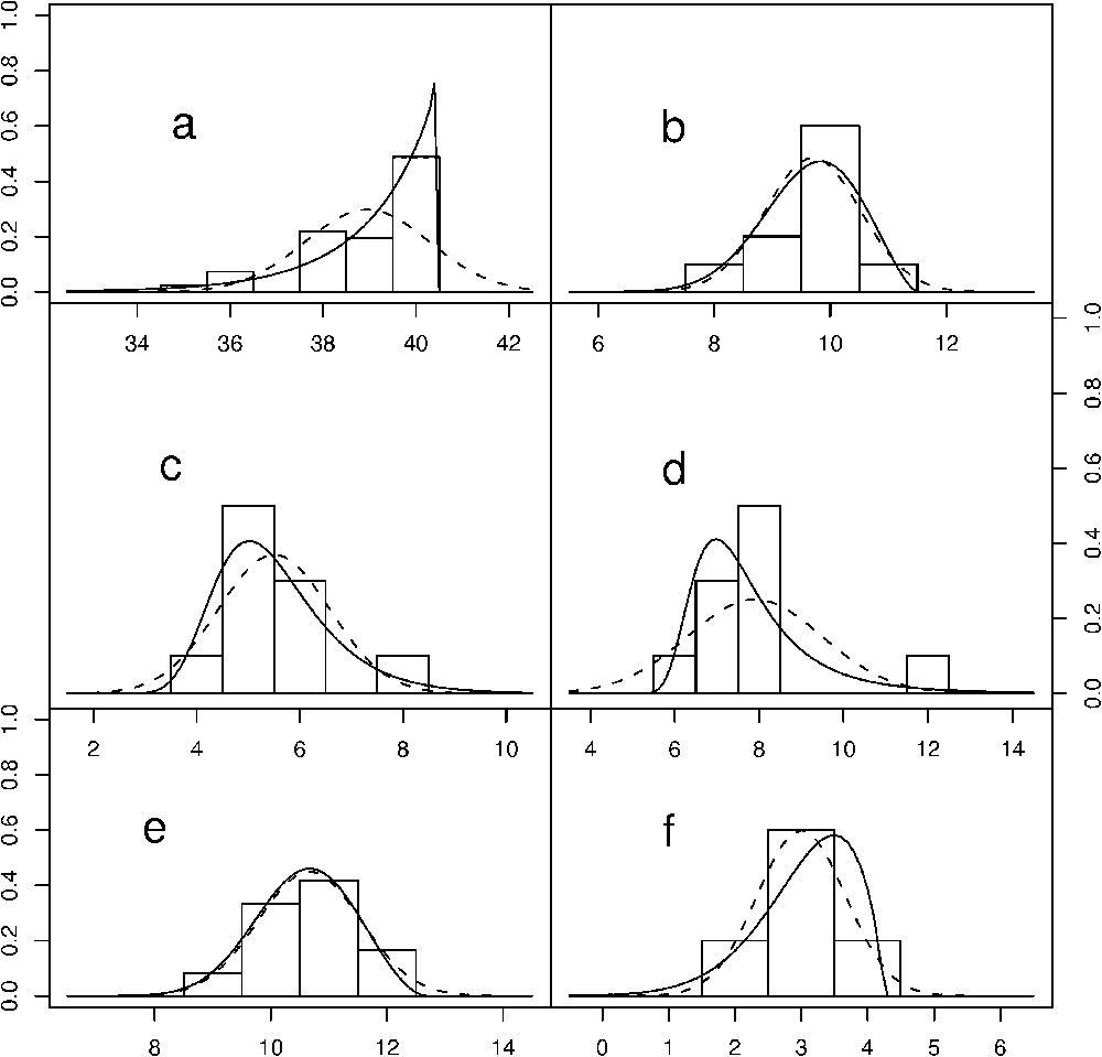
Distributions of maxima lichen diameters (cm) from 6 moraines near Mt. Charquini (Bolivia). The dotted line shows the fit by a Gaussian density. The solid line indicates the fit by a Generalized Extreme Value density.
Les distributions des diamètres maximals de lichen provenant de 6 moraines près du Mont Charquini en Bolivie. Les lignes en pointillés représentent la courbe obtenue sous l'hypothèse d'une loi gaussienne. Les lignes en trait plein correspondent à la courbe obtenue sous l'hypothèse d'une loi Généralisée des Valeurs Extrêmes.
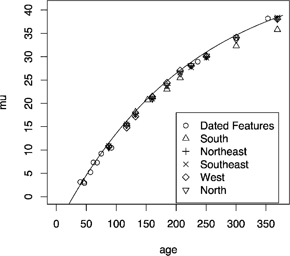
The mean age versus the mean μ parameter with an exponential growth curve model. The dated features correspond to measurements taken generally from nearby dated places such as bridges, tombstones, etc.
Courbe exponentielle entre l'âge moyen et la moyenne du paramètre μ. Les caractéristiques datées correspondent à des mesures ayant été obtenues à l'aide de marqueurs temporels, tels que les ponts, les tombes, etc.
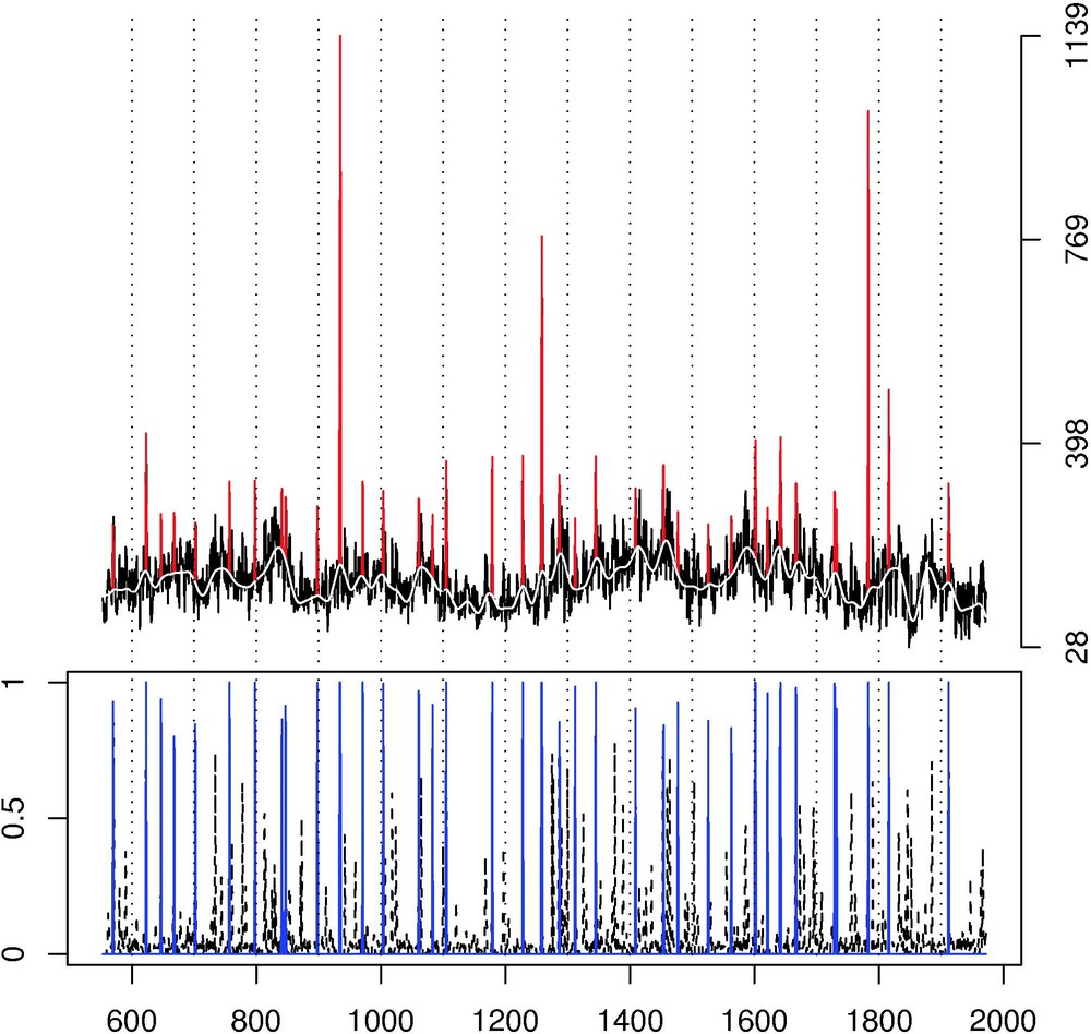
Bottom panel (x-axis = years): The probabilities (y-axis) were derived from an extraction procedure described in [22]. The blue solid lines represents the detected events with an associated probability larger than 0.8. Top panel: Crete ice core of South-Central Greenland [12]. The red peaks correspond to the detected peaks (see the lower panel).
Panneau inférieur (abscisse = année) : Les probabilités ont été obtenues à partir d'une procédure d'extraction décrite dans [22]. Les lignes bleues représentent les évènements ayant une probabilité d'occurence supérieure à 0,8. Panneau supérieur : ‘Crete ice core of South-Central Greenland’ [12]. Les crêtes rouges correspondent aux crêtes détectées (voir le panneau inférieur).
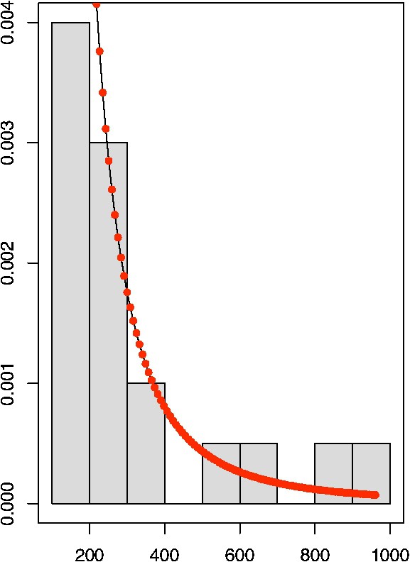
Histogram and the fitted GPD density (see Eq. (2)) for the extracted exceedances obtained from the top panel of Fig. 3.
L'histogramme et la courbe ajustée par une densité GPD (voir l'Éq. (2)) pour les crêtes obtenues à partir de la Fig. 3.
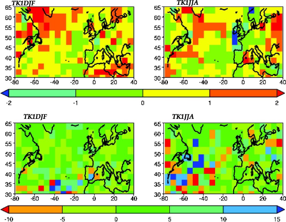
Two top panels: 30-year return levels changes (in degrees Celsius) of extreme daily temperatures. Two bottom panels: 30-year return levels changes (mm/day) of extreme daily precipitation. For all graphs, the left column corresponds to the winter (December to February), and right column to the summer (June to August). The return levels change is defined as the difference between the return levels computed after and before the THC jump.
Figures supérieures : Changements dans les temps de retour à 30 ans pour les températures extrêmes journalières (en degrés Celsius). Figures inférieures : Changements dans les temps de retour à 30 ans pour les précipitations extrêmes journalières (en mm/jour). Pour chaque graphique, la colonne de gauche correspond à l'hiver (de décembre à février), tandis que celle de droite représente l'été (de juin à août). Un changement dans les temps de retour est défini comme la différence entre les temps de retour calculés après et avant le saut THC.
1 Introduction
In recent years, there has been a growing interest in extreme events such as droughts, heat waves, etc., within the climate community. By definition, extreme events are rare but they do still occur and records are eventually broken. Hence, one may like to know if new climatic records like the European heat wave in 2003 or the 1999 winter storms in France occurred by ‘chance’ (i.e. in a random way) or if they are due to the human-induced climate change or other non-stationary phenomena. Currently, the statistical community is not able to provide a multivariate spatio-temporal theory that can completely model the distribution of extremes in complex systems like our climate, and consequently to fully answer such questions. However, there exists a basic theory for extremes that can help the climatologist to perform simple statistical analyses related to extremes.
In this paper, we first recall the principles of extreme value theory (EVT) and then apply them to three different case studies: lichenometry, volcanic forcing and the simulated atmospheric impact of an ocean circulation change. Besides their relevance to climate, the common point between these topics is that EVT can improve their analysis. The lichenometry study is performed by linking maximum lichen diameters with moraine ages. A characterization of strong volcanic peaks is proposed in order to better model the volcanic forcing in climate proxies. Finally, the impact of an abrupt change in the thermohaline circulation in a climate model is studied by analyzing the behavior of extreme temperatures and precipitation before and after the prescribed shift. These three case studies will exemplify the universality of this theory and will demonstrate that EVT could become a powerful tool for the practitioner who wishes to go from some simple exploratory data analysis methods to a more complete and parametrized statistical model. The last step is important when deriving confidence intervals and understanding of what assumptions were made in an error analysis.
EVT is the branch of statistics which describes the behavior of the largest data observations and it has a long history going back to 1928 [10,11,25]. It has been applied to a variety of problems in finance [9] and hydrology [17]. Surprisingly, its application to climate studies has been fairly recent. For example, in 1999, an entire special issue of the journal Climatic Change [15] was dedicated to weather and climate extremes but the EVT was rarely mentioned or applied. Fortunately, in the last 5 years, climatologists have been more inclined to take advantage of this theory, e.g. [18,27]. This paper can be regarded as a further step in this direction.
2 Analysis of maxima
The historical cornerstone of EVT is the generalized extreme value (GEV) distribution which classically models block maxima. The justification for the GEV distribution arises from an asymptotic argument. As the sample size increases, the distribution of the sample maximum, say X, will asymptotically follow either a Fréchet, Weibull, or Gumbel distribution. Similarly to many results in mathematics and physics, a stability property is the key element to understand EVT. More precisely, suppose that represents the maximum of the sample . One may wonder which type of distributions are closed for maxima (up to affine transformations). This requirement is equivalent to find the class of distribution that satisfies the identity in law for some appropriate constants and . The solution of such an equation is called the group of max-stable distributions. Intuitively, this means that if the rescaled sample maximum converges in distribution to a limit law, then this limiting distribution will have to be max-stable. The distributions (Fréchet, Weibull and Gumbel) are the only members of this group. This explains why the statistical modeling of maxima can only be based on these three distributions that can be described by the more general GEV distribution defined by
| (1) |
In this paper, all our model parameters are obtained by implementing a maximum likelihood estimation procedure. To illustrate this method, we look at the GEV distribution defined by (1). In this case, the likelihood is the probability of observing our given maxima that are assumed to follow a GEV density whose parameters are unknown (see [6] for more details). In order to estimate these parameters, it is reasonable to choose the parameters that maximize the likelihood with respect to our data. More precisely, the following steps need to be implemented: (a) compute the GEV density by differentiating (1) with respect to x, (b) write down the likelihood function for the sample , i.e. calculate the product of n densities evaluated at each , (c) maximize the likelihood function with respect to the unknown parameters . One of the advantages of using a maximum likelihood estimation procedure over other techniques is that it offers a lot of flexibility, e.g., if more complex statistical models with explanatory variables have to be studied. The next section illustrates these advantages by applying EVT to the field of lichenometry.
2.1 Lichenometry, LIA and maxima
The Little Ice Age (LIA), a period stretching over several hundred years from about 1300 to 1850 AD during which several episodes of persistent (cool) climate anomalies occurred, had important implications for human activities during this time period. One may wonder if such a climatic phenomenon was specific to Europe, or if other parts of the world, or the entire globe, experienced similar perturbations. One area with previously relatively limited data that could help answer these questions is the Southern Hemisphere. Here we focus on the South American Andes from which a host of new results have become available [23,24]. More precisely, glacial variations have been recorded by moraine formations that mark advances and retreats. Hence, in the context of gaining a better understanding of the timing of the LIA in South America, one opportunity for dating moraines and glacier retreats is offered by lichens. These simple organisms grow uninterrupted for many centuries. For these reasons, lichenometry, the study of using lichen measurements to determine the ages of glacial landforms, was introduced by Beschel in the 1960s [1]. A fundamental assumption of lichenometry is that the largest lichens found on a moraine are also the oldest ones on the moraine. Consequently, lichenometers employ only the largest lichens while in the field. In our case, a large number of maximum lichen diameters per block were obtained around Mt. Charquini in Bolivia. A more complete description of this region and this technique can be found in [24]. Hence, the very nature of the data imposes that EVT should be used in lichenometry studies. However, EVT has been rather absent from past lichenometry error analysis. Classically, the distribution of the largest lichen sizes was incorrectly assumed to be near normally distributed (see, for example, Figs. 2 and 7 in [20]). A few authors noticed this discrepancy between the maximum distribution and a Gaussian fit. For example, Karlen and Black [16] made use of the Gumbel distribution, but they did not take full advantage of the EVT (the Gumbel density being only a special case of the GEV density). To illustrate this point, we plot in Fig. 1 the histograms of maxima for different moraines. It is very clear from panel (a) that the fit by a Gaussian density (dotted line) is too restrictive to accurately represent maximum lichen sizes. In comparison, the fit by a GEV density (solid line) provides a much better agreement for all the sampled moraines. It is important to note that the fit of maxima by the normal distribution is not theoretically sound from a probabilistic point of view and it does not offer the flexibility necessary to fit all the maximum distribution cases, in particular when an asymmetry is present. At this stage, the fit of maximum diameters by the GEV has been performed. However, the primary variable of interest in lichenometry is the moraine age, and thus the date of the glacial advance, but not the lichen diameter per say. Hence, a growth function linking the moraine ages with maximum lichen diameters has to be constructed. Prior knowledge from geomorphologists indicates that the lichen growth is reasonably modeled by an increasing and concave down function. This behavior is due to the faster growth of younger lichens and the slower rate for older ones whose diameters tend to plateau as their ages increase [14]. To accommodate this physical phenomenon, we propose to allow the location parameter μ from the GEV modeling in (1) to vary in function of the moraine age as where δ represents a given age and the αs correspond to unknown parameters to be estimated. The estimated parameters for this growth curve are only valid for each individual glacial lobe. To add the flexibility to pool measurements from different nearby glaciers (hence reducing the error margin), it is possible to develop a Bayesian hierarchical model [5], i.e. the parameters like μ and the α's are not fixed but are considered as random variables whose distributions can represent spatial structure or other mechanisms. Such complex models are common in statistics whenever the randomness of the system occurs at different scales. With this approach, we estimate the posterior mean of μ (μ being now a variable it is possible to estimate its mean) by pooling five different glaciers surrounding the Charquini region (see Fig. 2). The details of such a statistical modeling can be found in [7].
Besides being based on a sound mathematical theory, the advantage of using the GEV distribution over past approaches is that this model can provide credibility intervals to assess the uncertainty associated with age and other parameter estimates, while keeping a flexibility that allows for different growth curves and spatial relationships to be fitted.
3 Extreme value theory for exceedances
In an extreme value context, data points are by nature scarce. This means that the uncertainty is large. Hence, any approach that reduces this uncertainty is very valuable. In the previous example, a Bayesian framework enabled us to pool maxima from different glaciers. Another strategy is to model exceedances above a large threshold instead of working with maxima. Indeed, modeling only block maxima is a wasteful approach to extreme value analysis if all the samples are available. This was not the case in the above lichenometry example where only maxima were recorded in the field. Of course, one difficulty is to define the word ‘large exceedances’. The following probability theorem clarifies this term.
Similarly to the theory for maxima, we know that the distribution of large exceedances above some threshold t is not arbitrary but it can be asymptotically approximated by the Generalized Pareto distribution (GPD), i.e.
| (2) |
3.1 Volcanic forcing on climate
Large explosive volcanic eruptions can play an important role in climate over the range of a few years [8]. Their typical spike-like signature has been found in numerous long climatic time series, instrumental and proxy alike [3,4]. Statistically, they can be viewed as pulse-like events, i.e. short and intense deviations from the background climate. Recently, a new method has been proposed for an automatic extraction of pulse-like signals [22] which offered the advantage of being an objective procedure to identify the timing of events. Additionally, a probability associated with each extracted event provided a measure of confidence in the extracted pulse-like event, see bottom panel in Fig. 3. In this paper, our goal is to characterize the magnitude of the extracted extreme signal (only the largest of explosive eruptions inject significant amounts of gases and aerosol into the stratosphere). These very large spikes clearly do not follow a Gaussian distribution but rather a skewed one that can take values outside of the range of a exponential tail, e.g., the Tambora eruption in 1815. Hence, the GPD should provide a theoretical framework for fitting this distribution. To confirm this claim, we study a time series from the Crete ice core of South-Central Greenland [12] that is the result of an electrical conductivity measurement (ECM) that records the concentration of highly conducting substances such as acids. These include sulfuric acid, the major aerosol produced by large volcanic eruptions.
As described above, the theory states that if a sufficiently high threshold t is applied, exceedances above this threshold must follow a GPD. Classically, finding an optimal threshold is a difficult problem. A value of t too high results in too few exceedances and consequently high variance estimators. For t too small, estimators become biased (the theory works only asymptotically). For our cases, the pre-selection step of only keeping pulse-like events with a posterior probability of greater than 0.8 (see blue lines in the bottom panel of Fig. 3) is equivalent to remove lower values. Consequently, we are already working in the tail of the distribution and the threshold selection is less important, as the approximation of the exceedances by a GPD is reasonable here. Still, to optimize the threshold choice, we implement classical threshold selection methods: mean excess function, thresholds versus parameters. See Section 6.5 of [9] for more details on these techniques. To assess the final quality of fit between the GPD and this data set, the GPD density is superimposed to the histogram of the exceedances in Fig. 4. Other diagnostic tools [6] to assess the GPD fit quality (qq-plots, etc.) have verified our approach. The fit is good overall and the largest values are captured by the estimated density. This will not be the case with a simple exponential function [13], and even less with a Gaussian fit. The estimated shape parameter is clearly positive ( with a standard error of 0.37) and it indicates that the distribution of exceedances is heavy tailed. This tail behavior has been confirmed with other proxies [21]. Such a result could be used for detection and subsequent attribution of natural climate forcing over the past centuries and millennia and provides a parameterization to generate realistic forcing series for climate model simulations with statistically appropriate forcing scenarios.
3.2 Impact of a THC jump on extremes
In this section, we investigate the impact of a prescribed abrupt mean change in the northward heat transport associated with the thermohaline circulation (THC) on climate variability around the North Atlantic. To this end, a 200 year control simulation run of the low-resolution IPSL-CM2 coupled ocean–atmosphere model [2,19] is analyzed. This simulation, forced by modern pre-industrial conditions, offers the peculiarity of a sudden jump of the THC (from 15 Sv to 30 Sv) after 120 years into the integration. This jump corresponds to a shift of the deep ocean convection zones from the Greenland–Iceland–Norwegian (GIN) Sea to the Labrador Sea. Hence, two states of the THC are identified and labeled as ‘before’ and ‘after’ the jump. The question we then address is what is the sensitivity of temperature and precipitation variability with respect to the THC change? While the mean behavior of these two variables seems rather unaffected by the jump in North Atlantic region (except in the oceanic convection zone, figures representing the mean fields are available upon request), it appears that the amplitude of extreme events are much more sensitive to the THC change. To precisely quantify these extreme temperatures and precipitation variations, we want to fit a GPD distribution to exceedances for these two variables. Because manually selecting a separate threshold for each of the gridded data points is impractical, the threshold is automatically set as the 90th percentile for each grid point. Due to the inherent seasonal cycle in the data sets, it is also necessary to separate winter and summer periods in order to compute climatically consistent extremes. Therefore, we focus on temperature and precipitation exceedances over the winter (December to February) and summer (June to August) periods. The final technical issue is to find an adequate summary of the three GPD parameters for each grid point. This task can be easily performed by introducing the concept of return levels, which also has the advantage of being interpretable and well known by hydrologists. Mathematically, we say that is the return level associated with the return period T whenever the level is expected to be exceeded on average once every T years. After estimating the GPD parameters, it is easy to compute for each location. In this paper, T is chosen to be equal to 30 years. Fig. 5 displays the difference between the return levels computed after and before the THC jump. Panel (a) corresponds to extreme temperatures. The amplitude of the return levels change is generally less than 2 °C, but it can be locally higher than that of local mean change, especially away from the THC shift zones where the mean temperature hardly varies. In particular, a few zones around the North Atlantic have a larger sensitivity to the extremes changes than of the mean ones. In comparison, panel (b) is dedicated to the analysis of daily extreme precipitation. It shows the high sensitivity of precipitation extremes with respect to the THC jump, with higher maxima in the winter and lower maxima in the summer over the Atlantic and North America. Those structures can be explained by changes in the probability distributions of the regimes of atmospheric circulation [26]. A much more detailed analysis of the impact of the THC jump on extremes can be found in [27].
4 Conclusion
By studying three very different case studies, we show that extreme value theory can provide relevant answers to a wide range of questions related to climate extremes. With the first example dedicated to lichenometry, a Bayesian model based on the GEV distribution displays a better representation of the growth curve of glacier retreat in South America. This could lead to a better understanding of the Little Ice Age in this region. Our second application focuses on characterizing the magnitudes of very large volcanic eruptions in proxies. Fitting large peaks with a GPD distribution clearly indicates that the volcanic forcing on climate should be better modeled by an heavy tail distribution. In the last case study, the analysis of a coupled simulation presenting an abrupt increase in the thermohaline circulation shows an important change of the extremes in the atmosphere, temperature and precipitation alike. This behavior would not have been immediately recognized based on the mean climate response to the THC change alone.
Finally, we would like to conclude with a note of caution. Modeling extreme event distributions is by nature associated with a large margin of error. Again, extreme events are, by definition, rare and therefore very few large values are available to estimate the appropriate parameters. Extreme value theory helps by providing theoretically sound models. Still, the estimation procedure is performed on a very small sample. Without this limitation in mind, misleading conclusions can quickly be made. This is particularly true when dealing with complex non-linear and non-stationary processes for which the statistical theory may not work.
Acknowledgements
The authors would like to thank the ‘Institut de France’ for the opportunity to present this research in this journal. This work was supported by the European grant E2C2, the NSF-GMC grant (National Science Foundation, ATM-0327936) and by The Weather and Climate Impact Assessment Science Initiative at National Center for Atmospheric Research that is sponsored by the National Science Foundation.