

1 Introduction
The rotating Earth is oblate, that is, it is slightly ‘flat’ in the North Pole–South Pole direction, compared to the slightly ‘bulging’ Equator. This is the result of the hydrostatic balance between the dominant gravitational force, which wants to pull the Earth into a spherically symmetric configuration, and the centrifugal force due to Earth's rotation, which wants to expel mass away from the rotating axis but in the end only manages to modify the Earth into an slightly oblate body.
Quantitatively, this oblateness is about 1 part in 300, which is very close (but see below) the ratio of the centrifugal force on the equator to the gravitational force. This is by far the Earth's largest deviation from a spherically symmetric body. There are certain thermodynamic, but secondary, processes that cause departures from the rotational-hydrostatic equilibrium. Sustained by the internal heat engine and manifested as external gravity anomalies reflecting lateral heterogeneity of internal mass distribution, these deviations are in general no more than parts per million in relative terms.
Yet all these deviations are not static or constant; they change with time. The rotation of the Earth is itself changing over geological time, and the aforementioned mass heterogeneities also vary on timescales upwards from millions of years. On more human timescales, there operates a myriad of dynamic processes that involve mass redistribution in or on the Earth, from tides to atmosphere–ocean circulations, to internal phenomena like earthquakes, post-glacial rebound and core flows. For the Earth, these changes are typically on the order of parts per billion at the largest [9,24]. The present article is a story about the oblateness in particular and how and why it changes with time, where we examine the geophysical implications.
2 The Earth's oblateness parameters and their inter-relationships
As long as the Earth is a 3-D body, we shall use the word oblateness to describe its off-spherical shape. Traditionally, the term ‘flatness’, or ‘ellipticity’, has been used; these names are imprecise because the Earth, of course, is not ‘flat’, and it is a 2-D geometric object only when we try to draw it on paper.
There are several parameters in use to describe the oblateness; each one has its significance depending on the application in question. For simplicity let's for the moment assume the Earth is axially symmetric, or a body of revolution and so essentially a 2-D body, which is a good approximation.
By equating the general expression of the spherical harmonic expansion of the external gravitational potential field V with that of the mass distribution of a body, one concludes that the spherical harmonic coefficients, or Stokes coefficients, of V are simply normalized multi-poles of the density function of the body [4,5]. When specialized, the degree-2 Stokes coefficients are related to the body's inertia tensor elements through a set of equations known as generalized MacCullagh's formulas. In particular, the degree-2 zonal (order 0) Stokes coefficient is given by:
| (1) |
We can express in the following form:
| (2) |
The ‘geopotential’ field is V, modified by the centrifugal potential, i.e. , where ω is the angular speed of Earth's rotation. If one approximates the equipotential surface, known as the geoid, to an oblate spheroid of revolution, then one obtains the geoid oblateness for the Earth which can be given by the Clairaut's first relationship (for a review, see [27]):
| (3) |
Two more concepts of oblateness can be defined at this point: suppose the Earth is under rotational-thermo-hydrostatic equilibrium. A hypothetical hydrostatic geoid oblateness representing an idealized Earth can be defined; to first order can be found by [18]:
| (4) |
Now let us examine the numerical values. m is known to be , or 1/288.371, close to 1 part in 300 or 1/300. According to Eq. (3), half of it contributes directly to the geoid oblateness f. For f, the remaining contribution comes from , which, of course, shares the same dynamic origin as m, i.e. Earth's rotation. is measured from satellite geodesy (see below) to a high accuracy, , about one third of 1/300. So, the two terms in (3) contribute almost the same amount to f, i.e., 50% each, and f itself becomes close to 1/300, at or 1/298.257. Finally, the dynamic oblateness H in Eq. (2) is observed to be or 1/305.456, again close to 1/300.
Are these matchings in values just fortuitous? From dynamical considerations, one can rightly ‘guess’ that all parameters should be on the order of m, which they indeed are. However, upon closer examination as follows, they do not necessarily have to have such similar values, so in a sense the latter is fortuitous.
For a reasonable Earth configuration, we should have because of its moderate sensitivity to the internal density profile, although it is well recognized that H would be somewhat less than f because of the smaller oblateness of the interior layers (due to smaller centrifugal force) and the higher density toward the center of the Earth (and hence proportionally lower importance in contributing to the moment of inertia) [27]. Putting this condition into Eqs. (2) and (3), we see the following: the two terms would contribute near-equal shares to f in Eq. (3) and hence all the values would be close to m or 1/300, only if .
The interesting, but certainly not out of the ordinary, fact is that, knowing and H in Eq. (2), the Earth in reality has , indeed almost exactly 1/3! This of course does not have to be the case, but one does expect a η value somewhat less than 0.4, that of a uniform-density sphere, for a ‘reasonable’ centrally-heavy, terrestrial planet body such as the Earth.
Based on the PREM Earth model (Preliminary Reference Earth Model [15]) derived from seismological data, the Earth should have an estimated hydrostatic of 1/299.66 [29], about 0.5% smaller than the observed. This corresponds to a hydrostatic of , about 1% smaller than the observed. On the other hand, Liu and Chao [21] formulated the relation between A, B and the two Stokes coefficients of degree 2 and order 2. Using the gravity-observed values for the latter, they get , amounting to 69.4-m difference in the equivalent geoidal semi-major axis and semi-minor axis on the Equator. Although only that of , this amount is comparable to the non-hydrostatic portion in , as pointed out by [17]. They concluded that the non-hydrostatic portion of the three principal moments of inertia A, B, C only describes a triaxial body and appears to have no preference in orientation. As far as the aforementioned excess oblateness over the hydrostatic value is concerned, this does not favor the notion that this excess oblateness is a remnant, lagging ‘memory’ of the past, as the Earth slows down due to the tidal braking.
3 Comparative planetology
For a contrast, let us compare the Earth with the giant planet Jupiter. Jupiter has a faster rotation and a much larger mass, and hence larger radius and gravity. Its . We can expect that the geoid oblateness f and the dynamic oblateness H to be similar to m, but not necessarily very close in value. The observed . Adopting second-order formulas [29], which are more accurate than Eq. (2), . Assuming rotational-hydrostatic equilibrium, (cf. Eq. (4)), indicating that, not surprisingly, Jupiter is somewhat more centrally-heavy than the Earth. The derived . We further expect that the geometric oblateness is the same as f, except possibly for some small departures from rotational-hydrostatic equilibrium.
In another extreme example, let us consider a non-rotating, uniform-density body not under hydrostatic equilibrium (hence the shape sustained by its internal material strength), such as an asteroid. Then there exists an analytical, but complex, relationship between the spherical harmonic coefficients of gravity and geometrical shape [7]. For the present discussion, let us further assume a special case where the body is a slightly oblate spheroid. Then, letting in Eq. (2), we have the geoid oblateness . Since the body is not under hydrostatic equilibrium, the geometric oblateness is not equal to f; rather, according to Eq. (9) of [7], it equals . Finally, the dynamic oblateness , when (for a uniform spherical body), equals , the same as the geometric oblateness, as expected.
4 Consequences of oblateness
We live in the Earth's gravity field, controlled by the dominant monopole term . We hardly notice any consequence of the oblateness of the Earth (or for that matter the rotational centrifugal force). However, dynamically, the Earth's oblateness is an essential element in our livelihood – it stabilizes our Earth's rotation. The Earth is ‘bombarded’ all the time by countless geophysical agents exerting external torques as well as internal torques or mass transports that exchange angular momenta. Yet its rotation axis hardly changes relative to the Earth-fixed geography. This is not true if it were spherically symmetric: then the crawl of a bug or a firing of a canon, for instance, would completely ‘tumble’ the Earth relative to the (spatially stationary) rotation axis [16,22]. On the other hand, it is well known from classical mechanics that the rotation of a body about its principal axis of the greatest moment of inertia (C) is a stable one. What prevents large shifts of the rotation axis from happening is the extra oblateness in the form of with the associated extra angular momentum, which is to be overcome by any geophysical agent that tries to shift the Earth's rotational pole positions. Since the oblateness itself is a consequence of the rotation in the first place, it can be stated that the rotating planet is self-stabilized.
A corollary of the above, but on a less dramatic scale, the Earth's dynamic oblateness under the tidal torques exerted by the Moon and Sun gives rise to the astronomical precession of the Earth's rotation axis in space, and hence is the deciding factor for the precessional period. That in fact is how the dynamic oblateness H is determined. On the same token, H acts as the restoring factor that prescribes the free wobble, known as the Chandler wobble, of the Earth's polar motion. The period of the Chandler wobble would be days if the Earth were a rigid body, but was found to be significantly lengthened by the Earth's non-rigidity, or finite elasticity [22].
As stated, the geometrical shape of the Earth largely conforms to the oblate geoid. Therefore, the mean equatorial radius and the mean polar radius of the geoid differ by as much as . In particular, the global sea level follows closely this oblate geoid, only undulating on top of the geoid geographically no more than 200 m peak-to-peak and temporally less than 10 m or so. The land topography undulates up to , but largely supported isostatically.
As such, the oblateness also affects various geophysical quantities. For example, in the space geodesy enterprise using near-Earth satellites, the oblateness term resides in all Earth surface geometry that locates the geodetic observatories and altimetric targets. Similarly, the oblateness prevails in the external gravity field that significantly affects the satellite orbits from which geodetic measurements are made. On the Earth surface, together with the centrifugal force field, the oblateness gives the surface gravity a slight latitudinal dependence which is actually the largest term in the surface gravity anomaly on the global scale. In another example, the Earth's elastic free oscillation modes (often excited by large earthquakes) see splitting in their otherwise degenerate characteristic periods due to Earth's oblateness and rotation, completely analogous in the atomic world to the Stark splitting and Zeeman splitting, respectively, as such splitting is determined by the symmetry properties common to different dynamic systems [2].
5 Historical Notes
Sir Isaac Newton, based on his law of gravitation and force laws, was the first to realize that the Earth under rotational equilibrium should possess a non-vanishing oblateness. The value of favored by him and given in the Principia was 230. Cassini subsequently came up with a negative value, −95, presumably owing to certain systematic errors. The value had evolved [19], since the Peru/Lapland expedition in the 1740s from a value between 179 and 266, to 301, 295, 297.0, and finally in the early 1950s to Sir Harold Jeffreys' which is within 0.4% of the modern value (298.257).
Then came the space age, ushered in by the launch of USSR's Sputnik I spacecraft in October 1957. A month later Sputnik II was launched, and within a few weeks, by monitoring the nodal precession of its orbit in space, our knowledge of grew almost an order of magnitude, to about 0.1% of the modern value. This measurement was arguably one of the very first scientific triumphs of space enterprise.
Today, after nearly half a century of precise orbit determination of dozens of geodesy-quality satellite orbits around the Earth, the Earth's global gravity field has been solved to harmonic degrees as high as 120, among which the average coefficient has been determined to the accuracy of seven significant figures () [20].
Since the 1980s, thanks to the advent of the technique of satellite laser ranging [1], tiny temporal variations around the average value of began to be noted. The variation occurs in the last digit of the above-quoted number and beyond, typically no more than one part in a billion! This will be discussed next.
6 How and why does Earth's change?
Mass transports in the atmosphere–hydrosphere–cryosphere–solid Earth–core system (the ‘Earth system’) occur on all temporal and spatial scales for a host of geophysical and climatic reasons [9,24]. According to Newton's gravitational law, such mass transport will cause the gravity field to change with time, producing time-variable gravity signals.
Increasingly refined models for the Earth's static gravity field in terms of spherical harmonic components have been determined by means of decades of precise orbit tracking data of many geodetic satellites. On top of that, low-degree components of Earth's time-variable gravity have been clearly observed by the space geodetic technique of satellite laser ranging (SLR) [1]. Although tiny in relative terms (no more than 1 part per billion), these variations signify global-scale mass redistribution in the Earth system.
In particular, the lowest-degree zonal harmonic is Earth's oblateness coefficient , whose temporal variation was the first to be detected among all gravity components. A ‘secular’ decrease in (over the observed quarter century) was first identified from the SLR satellite nodal precession acceleration. Its main excitation source has since been attributed to the post-glacial rebound (PGR) of the solid Earth [26,30], and for additional secondary causes [3]. Subsequently, many studies reported strong seasonal as well as weaker non-seasonal signals, primarily in , but of late also in the next-lowest harmonics [13] and geocenter. The prominent seasonal signals (with primarily annual amplitude ) have been correlated with mass transports in the atmosphere, oceans, and land hydrology [8,11,25].
Such was the case until around the turn of the century beginning in 1998, when the SLR data began to reveal that Earth's had suddenly deviated significantly from the PGR secular decreasing trend (at about ). This ‘1998 anomaly’ embarked on a reverse, increasing trend over the following years, before quieting back down to the ‘normal’ decreasing trend. This was reported by [10,12]. Fig. 1a shows an updated time series of the SLR-observed , using SLR data from up to nine satellites, with more satellites becoming available with time [12]. Note that the relevant 18.6-yr lunar-driven ocean tide amplitude was set to the value recovered in a 21-yr comprehensive solution for the secular zonal rates, low-degree static and annual terms, and the 18.6-yr and the much smaller 9.3-yr lunar tides. Fig. 1(b) is the same time series but after the removal of (i) the atmospheric contribution calculated according to the global NCEP reanalysis data assuming an inverted-barometer effect, and (ii) the least-squares fit of the remaining seasonal signals, which are attributable to (the poorly known) seasonal mass redistribution in the oceans and land hydrology. The PGR slope (the solid line) and the 1998 anomaly are clearly evident.
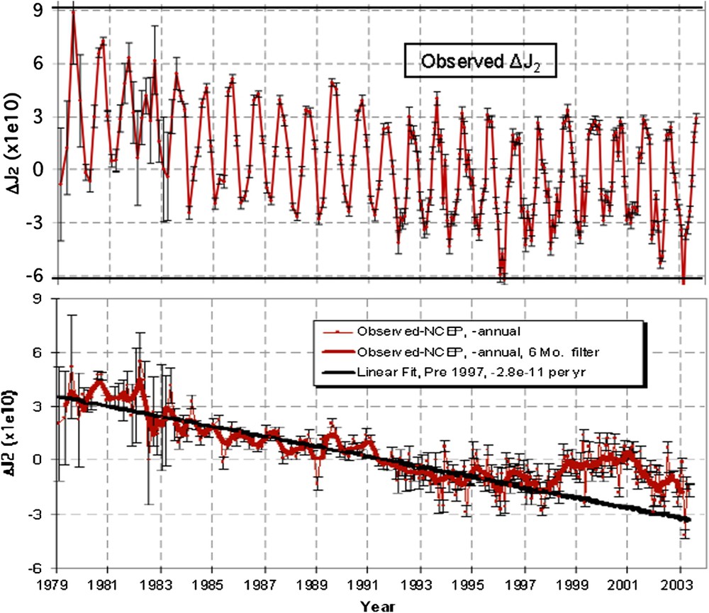
(a) Time series of the SLR-observed, non-tidal . (b) Same as (a), but after the removal of NCEP-calculated atmospheric contribution (with inverted-barometer effect) and any remaining seasonal signals.
(a) Variations temporelles de mesurées par les satellites laser (après correction des effets de marées). (b) Identique à (a), après retrait des termes saisonniers et de la contribution atmosphérique (calculée à partir des données de pression atmosphérique NCEP, dans le cas d'une réponse de type « baromètre inverse » de l'océan).
A number of possible causes for the 1998 anomaly was speculated by Cox and Chao [12], including oceanic water mass redistribution, melting of polar ice sheets and high-latitude glaciers, global sea level rise, and material flow in the fluid core. Dickey et al. [14] emphasized and demonstrated the importance of the melting of high-latitude glaciers. Chao et al. [10] report an oceanographic event that took place in the extratropic North + South Pacific basins that was found to match remarkably well with the time evolution of the anomaly; the phenomenon appears to be part of the Pacific Decadal Oscillation immediately following the episode of the 1997–1998 El Niño.
The difficulty in identifying the definite cause(s) in the above w.r.t. stems from the extremely low geographical resolution of the zonal harmonic function in question, namely the degree-2 Legendre function. Thus, a positive anomaly only tells us that a net transport of mass from higher latitudes to lower latitudes (across the nodal latitude of the degree-2 Legendre function, namely ±35.3°) has occurred, in either or both Northern and Southern Hemispheres. For example, an equivalent of as much as 3000 km3 of water melted from Greenland and spread into the oceans would be needed to produce the first half of the anomaly where the relative change is per year; but we have no way of telling without other ancillary evidences or observations. On the other hand, the space gravity mission of GRACE (launched in March 2002, with an expected lifetime of over 5 yr), using the satellite-to-satellite tracking (SST) technique, is yielding gravity information at much higher geographical resolution than the SLR-based information. For example, GRACE is able to detect centimeter level water-height-equivalent mass changes over an area of about 1000 km across from month to month [28]. However, considering the relatively weak sensitivity of the SST to the longest-wavelength (lowest-degree) gravity components, GRACE's utility in measuring the variation of in particular awaits to be seen. The same applies to future gravity missions of GOCE (using gravity gradiometer) and other SST measurements in ‘follow-on’ gravity missions under planning.
7 Relationship between Earth's rotation and change
As stated, the Earth's oblateness arises from its rotation; the rotational-hydrostatic relationship, to first order, is given in Eq. (4), where the oblateness is proportional to m, which is in turn proportional to . Therefore,
| (5) |
For example, the Earth's secular spin-down due to the tidal braking would lead to a secular ‘rounding’ of the Earth (barring possible temporal retardation under viscosity), thus decreasing . Numerically, at the tidal-braking rate of , that decreasing rate of is about , contributing only 2% of the observed decreasing rate of (see above).
On the other hand, any change in will cause ω to change, as dictated by the conservation of angular momentum for the Earth. For instance, a decreasing means a faster spin (analogous to a spinning skater pulling arms closer to the body), and vice versa. That effect can be shown to be [6]:
| (6) |
8 Epilogue
Although numerically small, the oblateness is a fundamental property of the Earth under stable rotation. Its existence and cause, its dynamical and geometrical consequences, its values and departures from idealized models, and its temporal evolution due to mass transports in the Earth system are all fascinating topics in geophysics, which reveal insights towards the understanding of the structure and dynamical behavior of the Earth. The measurement and monitoring of the Earth's oblateness have been a triumph as well as a scientific target of the modern space geodesy. As one sees deeper and finer into the Earth's oblateness, there is little doubt that the Earth will surprise and further fascinate us with a continuing story unfolding with time.
Acknowledgement
This paper is completed under the support of the NASA Solid Earth program. I am grateful to Christopher Cox for providing Fig. 1.