

1 Introduction
Estimation of the riverborne material flux (F) allows one: (i) to evaluate mechanical and chemical denudation rates [39,40]; (ii) to estimate output from catchment ecosystems and source apportionment between point and diffuse sources [1,16]; (iii) to evaluate nutrient and pollutant losses from river basins to coastal zones or lakes as required by international treaties (e.g., OSPARCOM: Oslo–Paris Commission on the North Sea; HELCOM: Helsinki Commission on the Baltic Sea, US–Canada treaty on the Great Lakes protection); (iv) to define and apply environmental objectives to restore and improve water quality, such as the Total Maximum Daily Load (TMDL) approach [33]; (v) to carry out a long-term analysis of annual flux in response to changes in land use activities and atmospheric deposition [10,14]; (vi) to assess the effects of best management practices (BMPs) in a watershed, as for heavy metals.
F is the product of the water discharge (Q) by the concentration (C). Due to variations in discharge as well as in concentration, obtaining longer-term loads, e.g., annual values, requires the integration of the instantaneous fluxes over the period concerned. Continuous records of water discharge are usually available, but river suspended particulate matter (SPM) and river-water chemistry variables are not: discrete water quality surveys are commonly carried out at weekly, biweekly, or even at greater intervals. They show that SPM concentrations at a given station range over two or four orders of magnitude [25,34], while major ions, organic carbon, nutrient concentrations and particulate pollutants contents in SPM generally range over less than one order of magnitude, even in impacted river basins [4,12,23,40]. The total phosphorus (TP) and total Kjeldahl nitrogen (TKN), which include both dissolved and particulate species, have an intermediate variability. Therefore, most riverine fluxes commonly range over two to four order of magnitude, depending on climate and basin size.
Several statistical or empirical methods related to riverine fluxes were developed in the early 1980s [7,8,28,31,36,37,39,41]. The reliability of flux estimates by these methods in the context of sampling strategies has long been the subject of much discussion and controversy. Two types of error are commonly defined [39]: bias (or systematic error), and imprecision (degree of dispersion). They were used: (i) to assess the potential reliability of loads calculated by various methods, such as the 22 algorithms reported by [29] and grouped into three classes (averaging estimators, ratio estimators and regression methods [30]; (ii) to demonstrate the influence of sampling strategies on flux imprecision [5,6,17–19,26,27,31]; (iii) to optimize sampling frequency or strategies (regular or stratified, discharge-based) for given imprecisions and bias targets [31].
Basin size is related to both the accuracy and precision of the individual load procedures for SPM fluxes [27,29], because it affects the SPM transport regime [25]. Other research has focused on the length of the estimation period, which also affects the errors of flux estimates [18]. Horowitz [11] shows that, for SPM fluxes, the very common approach using the ‘rating curve’, or regression method, tends to underestimate the high and overestimate the low SPM concentrations. Over periods of 20 years or more, a single rating curve based on all available data generates errors of less than 1%.
In our previous work on nitrogen and phosphorus on the eutrophic Middle Loire River, we compared the performance of seven algorithms for estimating annual nutrient loads based on near-daily surveys (four years) through simulated surveys at various frequencies [26]. We have also recently looked at riverine SPM fluxes using the discharge-weighted mean concentration method and their optimal surveys from a set of North American (N = 27) and European (N = 9) daily SPM stations, ranging from 600 to 600 000 km2 [27]. Our results show that the SPM transport regime of rivers affects the bias and imprecision of fluxes, for given sampling frequencies (e.g., weekly, bimonthly, and monthly). A flux duration indicator, the percentage of annual SPM flux discharged in 2% of time (Ms2), was found to be a robust indicator of SPM transport regime, on which a specific nomograph could be based, linking bias and imprecision of SPM fluxes to their survey frequencies [27].
In the present paper, we generalize this approach to seven other water quality variables in addition to SPM: dissolved and total nutrients and major ions (total dissolved solids, TDS, chloride) in four mid-sized rivers from the Seine and Loire Basins (France) and in two small tributaries of Lake Erie (Ohio, USA). We simulate water quality surveys with sampling frequencies ranging from 12 to 200 per year using Monte Carlo techniques, with the following objectives:
- • to establish flux uncertainties (bias and imprecision) for different water quality variables that present multiple C = f(Q) relationships;
- • to test the possibility of using the 2% duration flux indicator (M2 SPM for SPM, for nitrate, etc.) as a prediction of annual flux estimate uncertainties (interannual and annual level).
2 General methodology and database
2.1 Data sources, collection, screening
We have considered first four French basins (Table 1): two stations on the Middle Loire, operated by the Electric Power Authority Utility (EDF, Avoine station) and by the Loire Basin Authority (AELB, Orleans station), and three stations in the Seine River basins (Oise, Marne and Middle Seine), operated by the Mega Paris water-supply institution, SEDIF). For the Middle Loire, we used quasi-daily records taken during a pilot study from 1981 to 1985 for nitrate, orthophosphate, and total P at Orleans [26] and hourly records of conductivity and water discharge at the Avoine Nuclear Power Plant. For the Oise, Marne, and Seine Rivers, water quality (NO3−, NH4+, and conductivity) is monitored daily (1995–2004) at the Méry-sur-Oise, Neuilly-sur-Marne, and Choisy-sur-Seine water treatment stations, respectively. All these stations have a pluvio-oceanic water-discharge regime with winter high flows and summer low flows.
General basin characteristics, flow, SPM and dissolved regime indicators at selected French and US stations (Vw2, C50, C99, C*, M2, see text)
Tableau 1 Caractéristiques générales des bassins versants et descripteurs statistiques (valeurs inter-annuelles) des débits, flux de MES (SPM) et de matière dissoute (SRP, phosphore réactif soluble) aux stations françaises et américaines étudiées. TKN = azote Kjeldhal (Vw2, C50, C99, C*, M2 voir texte)
| Seine | Marne | Oise | Loire | Loire | Grand | Cuyahoga | ||
| WQ station | Choisya | Neuillyb | Méryc | Orléansd | Avoined | Painesvillee | Independencee | |
| Basin area (km2) | 30 710 | 12 710 | 16 972 | 36 970 | 56 480 (Langeais) | 1773 | 1832 | |
| Period of record | (1995–2004) | (1995–2004) | (1995–2004) | (1981–1985) | (1993–2003) | (1995–2003) | (1981–2003) | |
| Agriculture (%) | 58.7 | 69.2 | 71 | 54 | 58 | 40 | 30.4 | |
| Urban (%) | 4.9 | 4.2 | 6.0 | 1.0 | 1.0 | 0.9 | 9.6 | |
| Wooded (%) | 35.6 | 25.9 | 22.5 | 28.0 | 27.0 | 45.2 | 50.1 | |
| Other (%) | 0.8 | 0.7 | 0.5 | 17.0 | 14.0 | 13.1 | 9.9 | |
| Pop. density (p km−2) | 96.1 | 105.7 | 105.1 | 58.0 | 62.0 | |||
| Vw2 (%) | 7.3 | 7.2 | 7.7 | 10.3 | 10.2 | 17.2 | 12.2 | |
| SPM | C50 mg l−1 | 10.0 | 17.8 | 19.9 | 15.3 | 34.6 | ||
| C*/C50 [−] | 3.0 | 3.1 | 1.9 | 9.6 | 6.7 | |||
| C99/C50 [−] | 11.7 | 11.7 | 7.3 | 42.4 | 30.6 | |||
| M2 (%) | 25.2 | 20.6 | 17.5 | 57.2 | 46.9 | |||
| C50 mg l−1 | 24.9 | 20.8 | 21.4 | 7.2 | 1.8 | 10.2 | ||
| C*/C50 [−] | 1.0 | 1.1 | 1.0 | 1.1 | 1.6 | 0.7 | ||
| C99/C50 [−] | 1.4 | 1.6 | 1.3 | 2.0 | 4.2 | 2.5 | ||
| M2 (%) | 7.1 | 7.7 | 6.1 | 10.6 | 24.9 | 8.0 | ||
| C50 mg l−1 | 0.1 | 0.1 | 0.2 | |||||
| C*/C50 [−] | 1.1 | 1.0 | 1.0 | |||||
| C99/C50 [−] | 3.0 | 3.7 | 4.4 | |||||
| M2 (%) | 9.2 | 8.0 | 10.0 | |||||
| TKN | C50 mg l−1 | 0.5 | 0.8 | |||||
| C*/C50 [−] | 1.5 | 1.4 | ||||||
| C99/C50 [−] | 3.5 | 4.0 | ||||||
| M2 (%) | 26.9 | 22.5 | ||||||
| TP | C50 mg l−1 | 0.23 | 0.06 | 0.20 | ||||
| C*/C50 [−] | 1.2 | 2.3 | 1.6 | |||||
| C99/C50 [−] | 3.5 | 6.6 | 5.4 | |||||
| M2 (%) | 19.5 | 35.8 | 28.2 | |||||
| SRP | C50 mg l−1 | 0.09 | 0.01 | |||||
| C*/C50 [−] | 1.2 | 1.0 | ||||||
| C99/C50 [−] | 2.4 | 11.4 | ||||||
| M2 (%) | 13.4 | 23.1 | ||||||
| TDS | C50μS cm−1 | 450 | 493 | 589 | 283 | |||
| C*/C50 [−] | 1.0 | 1.0 | 0.9 | 1.0 | ||||
| C99/C50 [−] | 1.1 | 1.2 | 1.2 | 1.4 | ||||
| M2 (%) | 6.4 | 7.2 | 6.6 | 9.2 | ||||
| Cl− | C50 mg l−1 | 44.0 | 111.2 | |||||
| C*/C50 [−] | 0.9 | 1.0 | ||||||
| C99/C50 [−] | 3.3 | 4.3 | ||||||
| M2 (%) | 24.7 | 13.5 |
a SEDIF data, gauging at Alfortville (30,800 km2).
b SEDIF data, gauging station at Gournay (12,660 km2).
c SEDIF data, gauging station at Pont Maxence (14,200 km2).
d EDF data.
e Water Quality Laboratory of the Heidelberg College, Ohio, USA.
Conductivity is used here at a given station as a proxy for the total dissolved solids (TDS), as demonstrated for French rivers [20], and commonly used in water quality surveys [4]: as the ionic assemblage does not vary much at our stations, the correlation between conductivity at 20 °C (in μS cm−1) and the sum of major ions (Σ = Ca2+ + Mg2+ + Na+ + K+ + Cl− + SO42− + HCO3−), expressed in mequiv l−1, is linear and constant. For instance, for the Loire at Orleans: conductivity = 95,52 Σ (r2 = 0.9, n = 36) for a range of conductivity between 180 and 330 μS cm−1. We therefore consider throughout this study that conductivity at stations can be assimilated to the TDS (mg l−1), which we processed in the same way as nutrients and SPM.
Two US tributaries to Lake Erie are also selected to test our findings in river basins of different sizes (area < 2000 km2) and hydrological regimes (nivo-pluvial regime). The Cuyahoga and Grand Rivers are surveyed by the Ohio tributary Monitoring Program, operated by the Water Quality Laboratory of the Heidelberg College, Ohio [32]. Six water quality variables are considered: SPM, total phosphorus (TP), soluble reactive phosphorus (SRP), total Kjeldahl nitrogen (TKN), nitrate + nitrite nitrogen (‘NO23’) and chloride (Cl−). Records are daily and sub-daily during floods, up to three samples per day.
2.2 Data processing
Altogether, the database of daily records represents about 315 yearly records for eight water quality variables at seven different stations. We have systematically applied the same data processing for each of the water quality variables, according to the following steps. Full details can be found in [27].
2.2.1 Preliminary step: data selection and completion
The SPM data for the Seine, the Oise, and the Marne Rivers are less frequent than data related to dissolved material (96 to 186 measurements per year, 1995 to 2004). They have therefore been completed from the daily discharge data, taking into account the flood patterns and flood ranks within one hydrological year and our knowledge of daily SPM surveys in similar French rivers. This procedure was validated by actual daily SPM surveys over a three-year period at the Poses station (1983–1985) on the Seine River, of similar size and hydrological regime (A. Ficht, pers. commun., [25]), and by a flood stage study in 1994/1995 [13]. Paris megacity storm overflows may induce sub-daily variations of NH4+ and SPM concentration. Since the Oise, Seine, and Marne stations are located upstream of this influence from Paris, we assume that the sub-daily temporal variations in such middle-sized river basins can be ignored.
After visualisation of the patterns of concentrations vs. discharge for all studied stations, we eliminated from our analysis data for soluble reactive phosphorus (SRP) for the Cuyahoga River, which present incomplete time series.
2.2.2 Step 1: Calculation of a set of statistical indicators designed to characterize the variability of concentration, water discharge and river material flux [25,27]
C*: river material constituent concentration, inter-annual mean discharge-weighted value (mg l−1 and μS cm−1 for conductivity);
C50, C99: 50 and 99 percentiles of concentration over the whole period of record (mg l−1 and μS cm−1 for conductivity);
Vw2, M2: percentages of water volume (Vw2) and of SPM (Ms2, in our previous works [25,27]) or dissolved material (M2) discharged in 2% of the time over the whole period of record (%);
vw2 and m2: percentages of water volume (vw2) and SPM (ms2) or dissolved material (m2) discharged in 2% of the time for individual years (%).
2.2.3 Step 2: Calculation of the reference fluxes (Fref) from daily data of annual fluxes
| (1) |
2.2.4 Step 3: Simulation of regular surveys using Monte Carlo techniques
Variable p is the replicate rank up to 100 simulations. Twenty-eight different sampling intervals (2 ≤ d ≤ 30 days) were simulated for all stations. This interval is not perfectly regular in order to simulate the actual sampling strategy used in current water quality surveys (pseudo-equidistant sampling, e.g., no sampling on Sundays). For example, for monthly sampling, the sampling interval of a survey is generated by a normal law (mean: 30 days, standard deviation: 4 days) resulting in simulated intervals ranging from 18 to 41 days [27].
2.2.5 Step 4: Estimation of fluxes for simulated surveys by one averaging method: product of discharge-weighted mean concentration and mean annual discharge
This method (M18) is among the 22 methods tested by Philipps et al. [29], and very commonly used and recommended [5,18,19,26,27].
For a given station and a given survey year j, the estimated yearly flux Fj (t yr−1) is the product of discharge-weighted mean concentration and mean annual discharge:
| (2) |
2.2.6 Step 5: Determination of riverine flux errors
The yearly flux errors, ej(d, p) for each year j and sampling interval, (d), were evaluated, for each replicate p, using the following formula:
| (3) |
2.2.7 Step 6: Relationship between errors and duration indicators
Biases and imprecisions generated by the M18 method were analysed according to the metrics of concentration, discharge and flux variabilities (Vw2, M2, vw2, m2) for each station, sampling interval, and riverborne material.
3 Results
3.1 General levels and variability of concentrations
The Loire, Seine, Marne, and Oise Rivers, at their selected stations, are typical of medium-sized Western European Rivers, with pluvio-oceanic river regime (winter high waters, summer low waters), low SPM concentration, high nutrients and high total dissolved salts, expressed by electrical conductivity. The Grand and Cuyahoga Rivers, located in the western part of Lake Erie basin (Michigan, Indiana, Ohio), have a snowmelt discharge regime with higher SPM concentrations, lower phosphate and nitrate, but higher ammonia or total Kjeldahl nitrogen (TKN). Their levels of total dissolved salts is lower than in the rivers of the limestone-dominated Paris Basin, but their chloride levels are somewhat higher than those found at the Loire and Seine stations, probably due to the use of de-icing road salts. Both river basins sets are very much impacted by human activities [32].
Median concentrations (C50, Table 1) represent the general levels. In the Loire and Seine Rivers, nitrates and ammonia levels are among the highest in the world, well above the natural ranges observed in some other rivers in the world [24]. In the Loire River, high nitrogen levels are related to the livestock farming (52 bovine heads of cattle per square kilometre for the catchment at the Orleans station), to the fertiliser use on arable land (23% of the basin area at Orleans), and to a medium–low population density (58 inhab/km2). In the Seine River, nitrates originate mostly from fertiliser use and ammonia from urban sources (population density ranging from 100 to 150 inhab/km2 at the selected stations) [2].
Lake Erie tributaries catchments, located in northeastern Ohio, are more forested. The Cuyahoga River basin is also heavily populated and industrialized [32]. In the Seine as a great effort has been done to collect and treat domestic sewage, the major sources of nutrients are now diffuse natural and agricultural ones [21].
The major origin of chloride is de-icing salts, ahead of other anthropogenic sources. In the Seine River, Cl−, Na+ and originate mostly from anthropogenic sources both domestic and industrial; de-icing salts are secondary sources. In the Loire River, water quality is relatively less impacted by industrial activity [9]. When compared to a global river set in which SPM range from 5 to more than 5000 mg/l ([25]), the median SPM levels (C50), reported here, are within the low values for the Seine stations (10 to 20 mg/l) and within the median values for Lake Erie's tributaries (15–35 mg/l).
The variability of concentrations and fluxes is illustrated by the ratio of two percentiles of concentrations (C99/C50) and by the ratio (C*/C50) between the discharge-weighted concentration (C*) and the medians (Table 1). Based on C99/C50, the order of variability is the following (from the highest to lowest):
SPM Erie tributaries > SPM Loire–Seine > SRP Grand > TP and Ppart all > NH4+, TKN all ≥ Cl− Grand–Cuyahoga = NO3− Grand–Cuyohaga > NO3− Loire–Seine > ∑+ Loire–Seine
The order is not quite identical for the C*/C50 indicator: the SRP figure is less variable than for TP in the Grand River, and C*/C50 for NH4+ in the Loire and Seine Basins is much less variable than for the Grand and Cuyahoga Rivers. It is important to note that C*/C50 is inferior to unity for the Grand River's chlorides and for the Loire and Seine Rivers’ conductivities. This is an indication that high flows are characterized by lower ionic contents, a near-universal relationship [40]. The origins of water quality temporal variations are multiple and encompass both natural and anthropogenic factors, physical control, as dilution, and biogeochemical controls, as seasonal phytoplankton uptake, and they very much depend on the size of the catchment [21,22].
3.2 Flux duration patterns
Duration curves give the proportion of water volume or riverborne material fluxes discharged in a given proportion of elapsed time [25,27,38]. They are evaluated as cumulative percentage flux vs. cumulative percentage of time, based on ranked daily fluxes, beginning with the highest values. In this paper, we distinguish duration curves evaluated for each individual year and for the whole period of record. The proportion of the highest riverborne material fluxes and water volume reached in 1, 2, 5, 10, 25, 50% of time (M1, M2, M5, M10…, Vw1, Vw2, Vw5, Vw10…) are key indicators of riverborne material and water flux patterns at a given station. For river particulates, the proportion of fluxes transported during a given percentage of time is always much higher than the proportion of river flow. M2 has already been applied to river basins from 103 to 106 km2 [25], with very different hydrological regimes, including the Mediterranean and monsoon ones. M2 is more accurately defined than M1. M5 would not be convenient with values rapidly exceeding 99% for smaller basins (<1000 km2) and/or flashy flux regimes.
We have chosen here, as a duration indicator, the cumulated highest fluxes carried during 2% of time (M2, expressed in% of flux during the period of record), as suggested in [25] and used in a previous paper [27] for the suspended particulate matter. The M2 indicators are calculated here for all water quality variables (Table 1) and compared to the water flux transported in 2% of time (Vw2, Table 1). Lowest figures of M2 and Vw2 correspond to the least variable river fluxes, while the highest figures describe the most variable ones.
For the Loire and Seine Rivers, Vw2 = 10 and 7%, respectively. These figures are close to the lowest variability observed at the global scale for such river basins [25], while those of the Cuyahoga (12%) and Grand (17%) Rivers are within the medium variability in a global Vw2 range from 4.5% to 31% for basins of similar sizes (5000 to 50 000 km2) [25]. For the SPM fluxes, M2 duration indicator (M2 SPM) are in the medium part of the global range for the Loire and Seine stations (M2 from 18 to 25%), while those of the Grand (M2 = 57%) and the Cuyahoga (M2 = 47%) Rivers are in the higher values observed at the global scale for such basins: the minimum (7.9%) is recorded in the Somme River (France) and the maximum (66%) for the Eel River (California) [25].
At a given station, the flux duration indicators determined for dissolved nutrients (NO3−, NH4+, and SRP), major ions, particulate phosphorus, total phosphorus (TP), and total Kjeldahl nitrogen (TKN) are always inferior to the SPM flux duration indicator, for the same stations, and generally superior to the water flux indicator (Vw2) (Table 1). In some cases, they can be inferior to Vw2; this is the case for TDS at the four Loire and Seine stations and for nitrate in the Cuyahoga (Table 1). This reflects the prevalence of relatively low TDS at the highest flow, which is also characterized by C*/C50 < 1.0.
When flux duration curves are represented in a double probability scale, they are linear [24]. Two examples are featured in Fig. 1 for the Grand River (Q, SPM, TP, TKN, SRP, , and Cl−) and for the Oise River (Q, , , and conductivity) (Fig. 2). In general, these duration lines are parallel to the water-flow duration line. Duration lines related to total concentrations, i.e., combining dissolved and particulate matter, are closer to the SPM lines (see TP and TKN for the Grand River) compared to the duration lines of dissolved material, which are closer to the water flow line (see SRP for the Grand River, and for the Oise River). Chloride in the Grand River and conductivity (CDV, i.e., TDS) in the Oise River are both represented by duration lines below the flow duration ones. The nitrate duration for the Grand River is awkward and cannot be explained at this stage. These differences between river basins and between water quality descriptors are now considered for the flux errors analysis resulting from the simulation of various sampling frequencies.
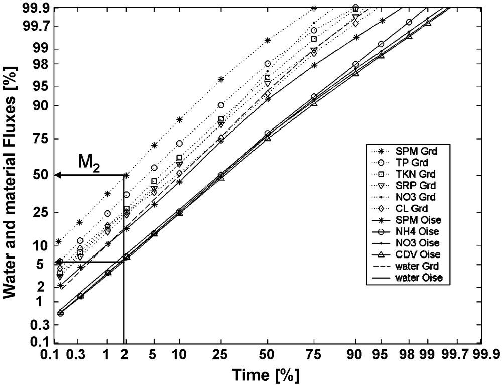
Patterns of daily water and river material fluxes duration vs. time duration for the Grand River, Ohio (Grd) and Oise River, France (Oise) (all constituents, inter-annual values). Double probability scale.
Fig. 1. Courbes de durées interannuelles des flux d’eau et de matière pour les rivières Grand (Ohio, USA) et Oise (France). SPM = MES, TP = phosphore total, TKN = azote Kjeldhal, SRP = phosphore réactif soluble, CDV = conductivité électrique, estimateur des sels dissous et totaux. Double échelle de probabilité.
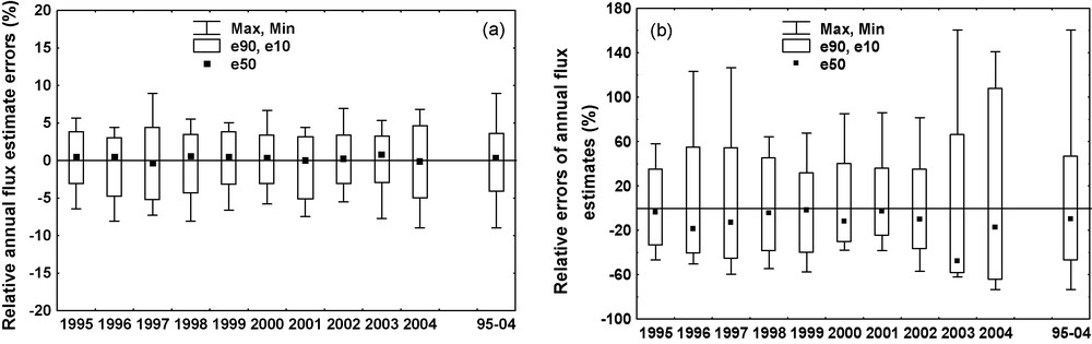
Distribution of annual and interannual flux errors using the discharge-weighted concentration method for the Seine at Choisy for simulated monthly surveys: (a) nitrate, (b) SPM.
Fig. 2. Distribution des erreurs sur les flux annuels (par année et interannuelles) avec la méthode de la concentration moyenne pondérée par les débits. Seine à Choisy, fréquence de suivi mensuelle : (a) nitrate, (b) matières en suspension (SPM).
3.3 Performances of discharge-weighted concentration: all constituents
The flux method based on discharge-weighted concentration (M18, [29]) is recognized to be less biased than many other procedures, for example, methods based on the time-weighted values of mean sample concentration (M14 and M17, [29]), but results in a large variability in flux estimations [39]. However, the M18 method is specified as the first choice of the OSPAR Convention, which deals with fluvial inputs to the North Sea [19]. We present here the flux estimate errors by the M18 for our dataset on SPM, TDS, nutrients, and chloride; then we test if the M2 SPM error nomograph, previously generated for the SPM fluxes [27], can be used to predict flux estimate errors for any riverborne material.
3.3.1 Biases and imprecision on annual fluxes for monthly surveys
For each water quality variable, we have simulated a set of 100 monthly surveys on which fluxes have been calculated by the discharge-weighted concentration method compared to the actual fluxes, determined on daily records.
The Seine at Choisy, surveyed from 1995 to 2004, is taken as an example. Fig. 2 shows the distribution, in box and whiskers plots, of the annual relative errors for each year: median (), lower deciles () and upper deciles (), and the maximum and minimum extreme errors.
Box and whiskers plots are also determined for the whole period of record (e50, e10, e90, and maximum and minimum). For a given sampling frequency, the annual flux errors using the discharge-weighted concentration method are very similar from year to year for nitrate (Fig. 2a), but very much less for SPM (Fig. 2b). For , the bias by method M18 is negligible and the imprecision is relatively minor (±5%), while SPM fluxes are generally biased and underestimated at all stations with biases reaching −50% in 2003. At such monthly frequency, many SPM flux calculations result in high imprecision (e90 − e10 > 50%). For ammonium, the imprecision is intermediate at all stations between that of SPM and NO3−; for TDS, imprecision is less than for nitrate, i.e. negligible (<±5% for monthly sampling).
In Fig. 3, flux estimates for a one-month sampling interval are compared for all water quality variables, at four selected rivers stations.
- • Bias and imprecisions are important for SPM, TP, TKN, NH4+, and minor for nitrate, TDS, SRP, and chloride. For example, for the Grand River, biases are −46% (SPM), −22% (TP), −13% (TKN), which is consistent with the decrease of the M2 duration indicator for these materials: 57% for M2 SPM, 36% for M2 TP, 27% for M2 TKN (Table 1).
- • For a given constituent, errors depend on the variability of concentrations with river discharge, and seem also related to the M2 indicator. For example, the imprecisions of annual nitrate fluxes are between 40 and 30% for the Grand and Cuyahoga Rivers (M2 around 24%), and only 8% for the Seine and Oise Rivers (M2 in the range 6 to 7%).
- • Biases and imprecisions are therefore very much station-dependent and river material-dependent for a given sampling frequency.
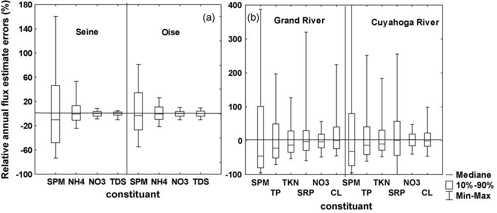
Distribution of interannual flux errors for simulated monthly surveys and various riverborne materials: (a) for the Seine and Oise Rivers (1995–2004), (b) for the Grand (1995–2003) and Cuyahoga Rivers (1981–2003).
Fig. 3. Distribution des erreurs sur les flux annuels de matière (échelle interannuelle, fréquence de suivi mensuelle) : (a) Seine à Choisy et Oise à Méry-sur-Oise (1995–2004), (b) rivières Grand et Cuyahoga (Ohio, USA, 1981–2003).
3.3.2 Biases and imprecision on annual fluxes according to sampling interval
The influence of the sampling interval on the interannual bias and imprecision of annual flux estimates for the whole period of record can be seen in Fig. 4 for the Seine and Grand Rivers and for the eight water quality variables. We are using here the bias and imprecision representation with a variable sampling frequency as used by [17] and already presented for SPM [27]. Biases are generally negative ones and increase with the sampling interval, as already noted in previous studies. For a given sampling interval (e.g., 20 days), the bias order is:
for the Seine River (Fig. 4a) and for the Grand River (Fig. 4b).
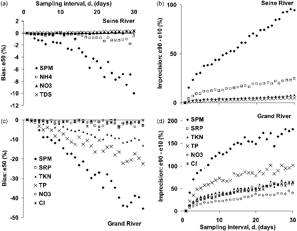
Interannual uncertainties (bias and imprecision) of annual flux estimates (method M18) according to the sampling interval for 8 variables (SPM, NH4+, NO3−, TDS, SRP, TKN, TP, Cl−): (a) bias, Seine River, (b) imprecision, Seine River, (c) bias, Grand River, (d) imprecision, Grand River.
Fig. 4. Incertitudes dans l’estimation des flux annuels (biais et imprécision, valeurs interannuelles) en fonction de l’intervalle de temps entre les suivis pour huit variables (SPM, NH4+, NO3−, TDS, SRP, TKN, TP, Cl−) : (a) biais, Seine à Choisy ; (b) imprécision, Seine à Choisy ; (c) biais, rivière Grand ; (d) imprécision, rivière Grand.
It must be noted that total nutrients (TP and TKN) biases are between those observed for SPM and those observed for dissolved material (Cl−, ). In addition, all Grand River biases are somewhat higher than the Seine River biases. At both stations, the bias order is very similar to the one observed for the flux duration indicator M2 (Table 1).
For all river materials, imprecisions increase rapidly with sampling intervals, between 2 and 10 days sampling intervals, then more slowly, between 10 and 20 days. Imprecisions are relatively low for all dissolved material compared to total nutrients and reach their maximum for river SPM. The order of imprecisions is similar to the one set up for biases. For the Grand River, all imprecisions are much higher than the one observed for the Seine River. For instance, imprecisions on nitrate fluxes are 25% for the Grand River and only 5% for the Seine River for a 20-day sampling interval. Such relationships enable to set up the sampling strategies when precision targets are set up.
3.3.3 Influence of the number of simulated surveys
The influence of the number of replicated surveys on flux errors is negligible. We are showing in Fig. 5 as an example the related interannual errors vs. sampling interval curves for SPM in the Grand River for four simulations: 50, 100, 500 and 1000 surveys for each sampling intervals. This is consistent with previous results obtained by [16] (50 simulations), by [15] (100 simulations) and by [3] (at least 150 simulations).
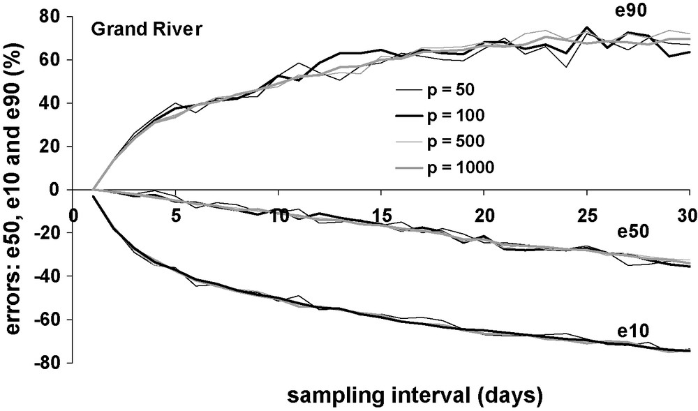
Evolution of interannual SPM flux errors (e10, e50, e90) for the Grand River according to the sampling interval and the number of replicates (p = 50, 100, 500, 1000).
Fig. 5. Évolution des quantiles des erreurs sur les flux annuels de MES (e10, e50, e90, valeurs interannuelles) pour la rivière Grand en fonction de l’intervalle d’échantillonnage (d, jours) et le nombre de tirages au sort (p = 50, 100, 500, 1000).
4 General relationship between errors and flux duration indicators M2 and m2
In a previous paper on SPM fluxes [27], we found a relationship between biases, imprecisions, and the flux duration indicator, M2 SPM, termed Ms2 formerly. We established a nomograph linking flux errors and M2 when using the M18 method on an interannual scale on 27 US stations and validated on a separate subset of nine European stations. We are here checking the flux errors–M2 relationships for other types of river material, i.e. dissolved material and total nutrients on our six stations (Table 1). These relations are first tested on an interannual basis for the whole period of record (on M2), then on individual years (on m2).
4.1 Use of a long-term flux duration indicator to predict flux errors at the interannual level (M2): monthly and weekly sampling
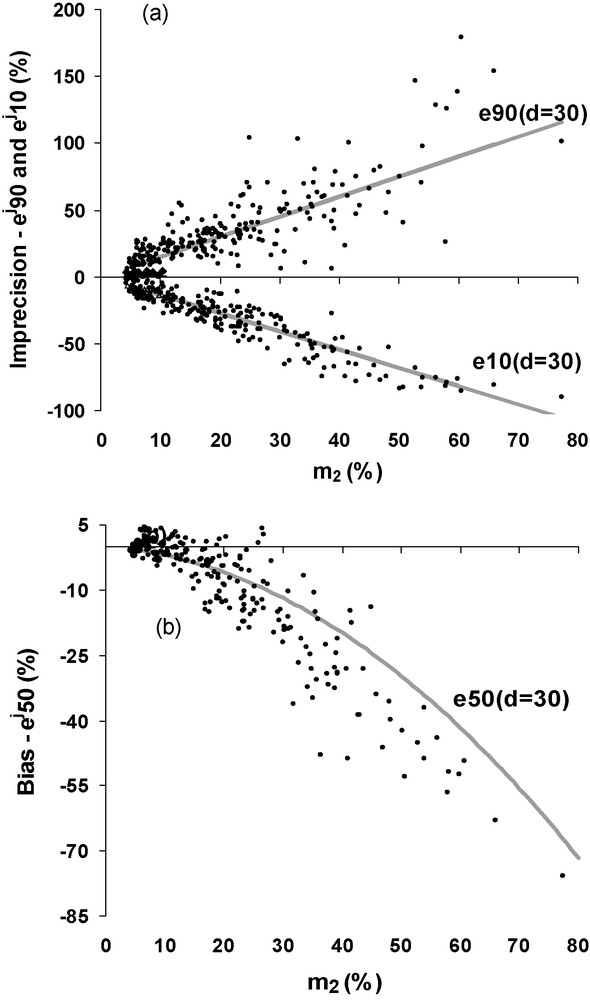
Altogether, we have a set of 23 flux error values, defined on e50 for biases, e10, and e90 for imprecision, for eight different water quality variables: SPM, TP, TKN, SRP, , NH4+, Cl− and TDS (conductivity), from simulated surveys over at least 10 years. All these errors are determined for the whole period of record and associated with the flux duration indicator for 2% of time (M2 SPM, M2 TP, etc, reported in Table 1) in Fig. 6 for two sampling frequencies: monthly (Fig. 6a and c), weekly (Fig. 6b and d). For nutrients and SPM, the three curves e10, e50, and e90 are those of the nomograph previously set up for the SPM only [27]. For Cl− and TDS, which are diluted at high flows, the bias could be slightly positive (zero to few percents for M2 < 10%) compared to SPM and nutrients biases, which are negative. For the imprecision (e10 and e90), the TDS data points also fit with the general nomograph previously established for SPM. We present here error nomograph parameters for monthly and weekly sampling intervals [27]: monthly, , e10=−1.36 M2, e90 = −1.50 M2, weekly, , , .
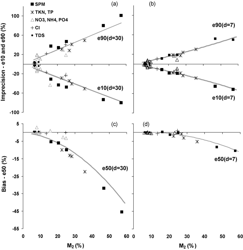
Distribution of relative interannual flux errors (upper and lower deciles, e90 and e10, median or bias, e50) for two sampling frequencies as a function of the long-term flux duration indicator: (a) imprecision, monthly sampling, (b) imprecision, weekly sampling, (c) bias, monthly sampling, (d) bias, weekly sampling. Data points: errors for the Seine, Marne, Oise, Loire, Cuyahoga, and Grand; all types of riverborne material (see Table 1). Curves correspond to the general nomograph based on M2 SPM only [27]
Fig. 6. Distribution des quantiles des erreurs sur les flux annuels (déciles inférieurs et supérieurs, e90 et e10, médiane ou biais, e50) pour deux fréquences de suivi en fonction de l’indicateur de durée des flux (M2 en %, valeur interannuelle) : (a) imprécision, fréquence mensuelle, (b) imprécision, fréquence hebdomadaire, (c) biais, fréquence mensuelle, (d) biais, fréquence hebdomadaire. Huit variables aux stations : Seine, Marne, Oise, Loire, Cuyahoga et Grand (voir Tableau 1). Les familles de courbes représentent les abaques antérieurs basés sur l’indicateur de durée M2, établis pour les MES seules [27].
For river SPM, there is a very good fit between the new set of measured errors (n = 5) and those predicted by the general M2 SPM nomograph that was expected. It is striking to note that biases and imprecisions for nutrients can also be well predicted by the same nomograph: the regressions for the new dataset are not significantly different from those of the nomograph.
The comparison between Fig. 6a–d confirms the major gains of accuracy and precision when sampling frequency increases from monthly to weekly. For a given M2 indicator, as an example 40%, the e90–e10 error range decreases from ±60% to ±30%, and the bias is even more reduced, from −22% to −5%. Such M2 values are commonly observed for river SPM in river basins between 1000 and 100 000 km2 [25,27].
Errors on fluxes of dissolved matter (TDS, Cl−, NO3−, NH4+, PO43−) are generally lower at our stations than those of total nutrients (TKN, TP) and particulate matter (SPM). These clusters are identified in Fig. 6.
The precision of riverine fluxes for a given riverborne material is very similar for the Oise, Seine, and Marne Rivers, which have similar hydrological regimes and concentration vs. discharge relations and basin size. Therefore, we believe that M2 indicators established at one pilot station for various types of river material can be used at the regional level for stations with similar hydrological and water quality regimes.
Interstation flux error variability is important for SPM, as already observed for a much larger sample of river stations [27], and decreases from SPM to TDS in the following order: SPM > total P and total N > Cl− > dissolved nutrients (N, P) > TDS. Since total P and total N are mixing both dissolved and particulate nutrients, their intermediate rank was expected. Chloride flux errors in Lake Erie's tributaries are here superior to those of dissolved nutrients due to the anthropogenic inputs of de-icing road salts that increase flux variability. This order of flux errors variability is similar to the one noted for the C*/C50 ratio determined on the long-term record at each station (see Table 1).
These types of interstation variability and inter-riverine material variability should now be confirmed on a larger dataset.
4.2 Use of the annual flux duration indicator (m2) to predict annual flux uncertainties
So far, most authors dealing with flux duration patterns have considered long-term series. This is particularly needed for daily suspended matter fluxes, which amplify the river flow variability, reaching three to four orders of magnitude [25]. For some rivers, the long-term average SPM flux can only be determined over longer periods, e.g., 20 years, including very rare floods that carry in a few days as much particulates as in a few years. The Eel River in California is one of the few documented examples of such a type [35]. In many rivers, annual fluxes are still reported on an annual basis, in order to comply with regional or international agreements. This is for instance the case of the OSPAR convention in the North Sea. Moreover, this annual reporting is also required for civil years that correspond to basin-management time steps, not for hydrological years, splitting winter high-water periods and their related fluxes into two successive civil years. Therefore, we are here testing the flux generalized duration nomograph for individual civil year and various riverborne materials based on the annual duration descriptors (m2).
We first consider the m2 indicators and their year–year variations for two-dozen surveys lasting 10 to 22 years (six river stations, eight riverborne materials, see Table 1). The upper and lower hand-fitted ranges of m2 include more than 95% of the data points. The m2 vs. M2 regression is: m2 = 0.922 M2 (r2 = 0.81, N = 280). For each riverborne material and station, the year-to-year m2 range is plotted against the long-term flux duration indicator (M2, see Fig. 7): the m2 range is very limited for the lower M2 and extends with increasing M2.
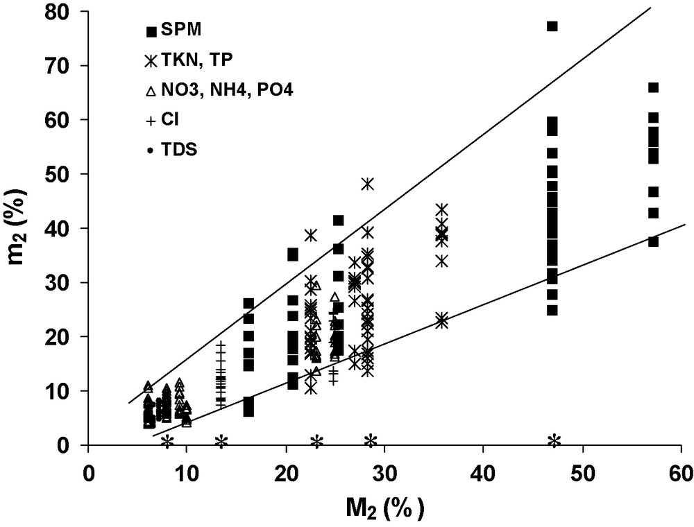
Annual flux duration indicator at 2% of time (m2) vs. long-term flux duration indicator (M2) for six stations and eight riverborne materials from total dissolved solids (TDS) to suspended particulate matter (SPM). (*): 22 years of daily records (Cuyahoga River), other sets are defined on 10-year daily records.
Fig. 7. L’indicateur de durée à 2 % du temps, évalué pour chaque année d’étude (m2) en fonction de l’indicateur de durée M2 (échelle interannuelle) pour six stations et huit constituants (*) 22 années de suivis journaliers (rivière Cuyahoga) et 10 années pour les autres stations.
The dispersion of annual flux duration (m2) observed at a given station and for a given material is directly linked to the annual water flow indicator (vw2), i.e. the proportion of water volume discharged during the seven highest ranked days of each civil year. Fig. 8 features such relationship for the total dissolved solids (three stations), TKN (two stations) and SPM (five stations). The m2 vs. vw2 correlation is excellent for TDS, fair for TKN and acceptable for SPM. It should now be confirmed for higher vw2 figures, particularly for dissolved solids.
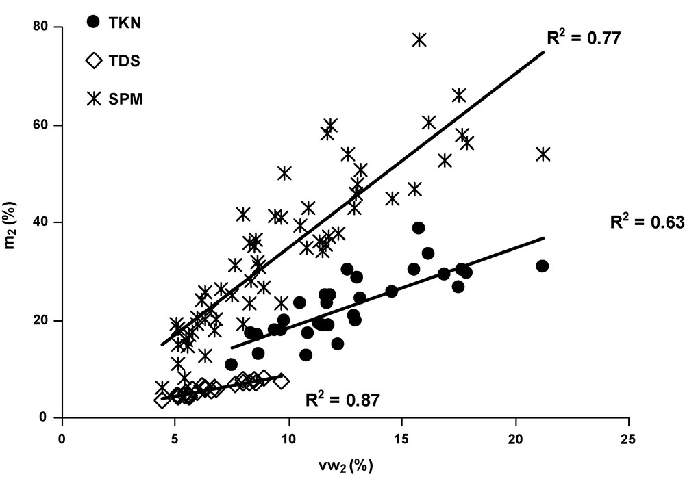
Relationship between annual flux duration indicators (m2) for three types of river material (TKN, TDS, SPM) and the water flow (vw2). SPM stations: Seine, Oise, Marne, and Loire Rivers; TKN stations: Grand and Cuyahoga Rivers. Ten-year surveys, except for Cuyahoga (22 years).
Fig. 8. Relation entre l’indicateur de durée à 2 % du temps (annuel, m2) pour trois type de constituants (TKN, TDS, SPM) et l’indicateur de durée à 2 % (annuel, vw2) du temps pour les flux d’eau. Matières en suspension (SPM) et sels dissous totaux (TDS) : stations Seine, Oise, Marne et Loire ; TKN : stations Grand et Cuyahoga. 10 années de suivi, excepté pour Cuyahoga (22 années).
We then test if the annual flux duration indicator (m2) can be used to describe the flux error distribution at the annual level. An example is given on Fig. 9 for the monthly sampling frequency. As for the interannual level, flux duration indicators at the annual level can be used to predict the lowest errors (ej10) and the biases (ej50). The prediction of the highest errors (ej90) is less outstanding, particularly for the SPM fluxes when m2 > 40%, but is acceptable for most dissolved fluxes with m2 < 20%. It must be noted that at such temporal scales, slightly positive biases can be observed for m2 < 20%. The general interannual M2 nomograph presented in Fig. 6 is also applicable at the annual level.
Distribution of relative errors (upper and lower deciles, and ; median or bias) for annual riverine fluxes determined from discrete monthly sampling as a function of annual flux duration indicators (m2). Combination of the Loire, Seine, Marne, Oise, Grand and Cuyahoga Rivers’ stations and of their riverborne materials surveyed during at least 10 years. Curves correspond to the interannual error nomograph [27].
Fig. 9. Distribution des erreurs relatives (déciles inférieurs et supérieurs, et ; médiane ou biais) sur les flux annuels déterminés à partir des suivis discrets mensuels, en fonction de l’indicateur de durée à l’échelle annuelle (m2). Stations sur la Loire, Seine, Marne, Oise, Grand et Cuyahoga, suivis pendant au moins 10 ans. Les familles des courbes représentent les abaques antérieurs établis à l’échelle interannuelle (M2) pour les MES seules [27].
5 Conclusions and perspectives
At the studied stations, the order of riverine fluxes precision is the following, from the best to the worst: TDS (total dissolved solids), nitrate, phosphate, total phosphorus, total Kjeldahl nitrogen, and suspended particulate matter. This order should now be confirmed on a larger dataset including other types of river regimes and of river material.
In river basins exceeding 1000 km2, the errors on long-term riverine fluxes using the discharge-weighted concentration method, associated with discrete river surveys, can be estimated with a single indicator, the percentage of long-term flux carried in 2% of time (M2 indicator). The general nomograph linking M2 with the lowest (e10) and highest (e90) errors previously established for river suspended particulate matter [27] can be used for other types or river material as major ions, dissolved nutrients, and total nutrients. For nutrients, which have a complex relationship with discharge, the median of the errors (e50) also fits the general nomograph. For those constituents, which are diluted at high flows as TDS and Cl−, the median of the errors can be slightly positive for low values of M2 (6 to 10%). This point should now be checked for those types of constituents for higher values of M2, which is expected to reach up to 20% for TDS in medium-sized catchments. The use of the nomograph is validated through the common range of sampling frequency from 2 days to 30 days and for M2 indicators ranging from 6% (least variable fluxes) to 55% (very variable fluxes).
Flux duration indicators, set up at the annual level (m2), present a year–year variability that depends: (i) on the riverborne material, with lower variability for dissolved substances and higher variability for substances partially associated with particulates, as total N and total P, and (ii) on annual water flow duration indicator (vw2). For instance, in middle-sized basins, the m2 indicator for SPM ranges from 15% to 40% for an average long-term value of 30%, typical of SPM fluxes.
When annual flux reporting is required, the generalized M2 nomograph established at the interannual level can also be applied to predict errors on annual fluxes (lower error, as decile , and bias, ) on the basis of m2 indicators, but for monthly sampling, the prediction of higher errors (e90) is poor when m2 SPM > 40%.
The statistical descriptors M2 (interannual) or m2 (annual) can be regarded as a measure of flux variability, more precisely of its dissymmetry. Therefore, flux imprecisions (distance between e10 and e90) are greater when M2 or m2 are higher. The practical application of the M2 nomograph is important, provided that M2 distributions are known regionally from pilot surveys at specific stations and then extrapolated for similar riverborne materials and stations. If such pilot surveys are unavailable, we believe that M2 can be derived: (i) from the combination of long-term water flow duration indicators as Vw2, which are available from daily records at any hydrological stations, (ii) from the structure of river material fluxes, e.g., quantile ratios of concentrations and/or fluxes, (iii) on concentrations vs. river discharge relationships, determined from long-term discrete samplings.
Acknowledgements
This work has benefited from financial support of the national ECCO programme (Variflux project) of the CNRS (France). This paper has greatly benefited from the use of the Lake Erie tributaries dataset, Ohio Tributary Monitoring Program (National Center for Water Quality Research, Heidelberg College, Ohio, USA). The SEDIF-CGE dataset for the Seine, Marne, and Oise Rivers were made available to us by Virginie Branchereau (SEDIF, Nanterre, France).