

1 Introduction and background
Numerous field experiments have shown that fluid flow and solute transport in highly heterogeneous fractured media mainly take place along preferential pathways within the fractures planes [1,25,29]. These paths or channels may represent less than 30% of the fracture plane volume [8,29]. Given this high flow heterogeneity, the classical continuous approach to the representation of fractured rocks, which is to model them as an equivalent porous medium, may become a poor approximation, at least for small and intermediate scales. The homogenisation scale, when it exists, is often larger than the size experienced by field measurements or/and numerical modelling exercises.
The stochastic discrete fracture network concept may appear much more adapted to simulate flow and transport at small and intermediate scales when channelled flow is expected. In two dimensions [2,24,32], and in three dimensions [26], it is proposed to model the channelling effects of flow at the fracture scale by discretizing the fracture plane conductivity according to statistical distributions. If this approach is a better representation of the local flow characteristics than homogenisation, a too large number of fractures can make it cumbersome for application at the block scale (say, 10 to 100 m) and, of course, hardly conceivable at the reservoir scale (one to several kilometres). To overcome this problem, some authors [9,10,15,20] proposed to write flow and transport equations at the channel scale. Three-dimensional fracture networks are generated by assuming (i) that fractures are discs, polygons or planes, and (ii) that channelling within fractures is represented by means of 1D pipes drawn at fracture intersections and between intersections and the centre of the fracture planes. This approach strongly reduces the number of unknowns when modelling flow and transport. However, as a drawback and contrary to what may happen in fracture fields, the 1D network is fixed once and for all. In fact, the flowing network will evolve with the mean head gradient's direction and/or the boundary conditions, but the price to pay is to handle (and compute) a huge network in which an important part of bonds corresponds to dead ends or non-flowing zones. As explained below, this drawback partly motivated the new approach proposed in this paper. Other approaches avoiding the representation of fractures have been considered. Some authors [17–19,21–23] studied flow and transport in a three-dimensional medium where regular bonds with high contrast of hydraulic conductivity are used together. Other authors [30,31] fitted the experimental breakthrough curves with a convolution of one-dimensional channels arrival times.
When dealing with pipe networks for modelling fractured rocks, two parameters condition the location of pipes: (i) the spatial distribution of the hydraulic conductivity in the fracture planes, (ii) the boundary conditions of the system. If the boundary conditions are for instance rotated around a block, the locations of flowing channels change accordingly [23] and both the main head gradient's direction and the channel orientations are then correlated. This paper proposes a new three-dimensional stochastic model based on the discrete pipe network approach, which is able to change channels according to the mean head gradient's orientation. The explicit representation of fractures is thus abandoned and the C++ code named MODFRAC3D generates three-dimensional networks of 1D pipes, whose orientations are conditioned by the head gradient's direction stemming from the boundary conditions applied to a 3D block. As is the case with other pipe approaches, fluid flow is assumed to occur only in fractures and the rock matrix is assumed impervious (or its flow is negligible compared to that in fractures). Fluid flow is simulated with a classical Eulerian finite-volume approach and mass transport is handled by the Lagrangian Time Domain Random Walk (TDRW) method [4,6,7,13]. This paper only deals with the pipe network simulation and incidentally with flow.
2 The approach
Basically, the approach used in this work to generate a pipe network differs from other Discrete Fracture Network (DFN) methods. Usually, DFN approaches drop planar objects (or bonds) in a Euclidean space with a possible conditioning of the objects on various features, e.g., length, density, orientation, etc. Intersections between the objects are in fact the consequence of the ‘bombing’. In the present case, the method for generating a pipe network is inspired from results of previous works at the scale of a single rough-walled fracture plane [16]. It has been shown that flow can be strongly channelled with a major part of water fluxes (say roughly above 75%) passing along very few narrow paths. In addition, it is often observed that some locations are crux nodes (designated as nodes hereafter) through which an important fraction of the flux passes, whatever the general orientation of the head gradient.
The main assumption triggering this work is the existence of such key nodes spatially invariant irrespective of the global gradient direction when flow channelling occurs. In addition, it is assumed, as for several DFN approaches, that channelled flow can be mimicked by a network of 1D pipes connecting these key nodes. To argue in this sense, a synthetic example reported below focuses on a 2D test at the scale of a rough-walled fracture plane.
A fictitious square fracture plane is discretized into a regular percolation network of 90 × 90 bonds (each bond is of size 1 [L]). An aperture sampled in a lognormal distribution (μ, σ in decimal log) is assigned to each bond. ‘Permeameter-type’ boundary conditions are applied at the edges of the regular network (no flow through the east and west limits, constant prescribed head of 1 and 0 [L] for the north and south limits, respectively). The steady-state flow equation is then solved in the fracture plane, and the equivalent macroscopic hydraulic conductivity is computed according to the following expression: Keq = Qin/|ΔL ΔH|, with Keq [LT−1] the equivalent hydraulic conductivity, Qin [L3T−1] the total inflow (outflow) through the north (south) limit, ΔL [L] the size of the system, ΔH [L] the difference between prescribed heads at upstream and downstream boundaries.
The flow rate through each bond is calculated to locate highly conductive bonds in terms of fraction of the total flow passing through the bond. It is arbitrarily considered that a bond is conductive if more than 1% of the total flow passes through it. A map of the major flowing paths is obtained, assimilated to the network of channels. The latter are kept, whereas the others are eliminated. The resulting network is assumed to correspond to channels in the fracture plane representative of flow for a north–south-oriented general head gradient. Another threshold of 30% of total inflow can be applied over this network for a north–south-oriented general head gradient and then repeated with an east–west gradient. Bonds over 30% of total inflow for both north–south and east–west gradients correspond to invariant key ‘nodes’ through which flow must pass. All the above procedure is repeated for different ‘fields’ of local hydraulic conductivity. The latter follows lognormal distributions of constant mean (μ = −5, in decimal logarithm) and standard deviation σ = 1, 1.5, 2, 2.5, 3, 3.5 and its spatial distribution is either fully random or correlated according to a spherical variogram of one-tenth the size of the system as correlation length. Maps of conductive bonds (above the 1% threshold) for σ = 1, 2 and 3.5 with correlated and uncorrelated conductivity are reported in Fig. 1. Bonds above the 30% threshold (i.e. indicating the location of key nodes) are in bold, whereas the rest, corresponding to flowing channels for a north–south-oriented general head gradient, are in light. A few comments can be drawn from a first look at the maps in Fig. 1a, corresponding to correlated conductivities: an increase in σ makes the most conducting bonds become connected and spatially concentrated, which results in flow channelling. As expected from intuition, this channelling with a few paths holding flow only occurs with correlated conductivities (Fig. 1b). Correlation in space yields clustered values of conductivity that are used as flow paths. Uncorrelated fields generate flowing bonds almost evenly distributed over the domain and non-channelled flows. It must be emphasised that this notion of channelling is empirical here, since it results from an appraisal ‘at first glance’ of the spatial distribution of flowing bonds. An attempt to define indexes of channelling can be done. For instance, invariant key nodes (above the 30% threshold) only appear in the case of correlated fields, which could sign the presence of channelled flow. Other measures are reported in Table 1. When conductivities are correlated in space, a more important part of flow is transferred by a less important part of bonds [23,31] (see the proportion of bonds above the 1% threshold) and the range spanned by local flow rate values is about ten times that from uncorrelated conductivities.
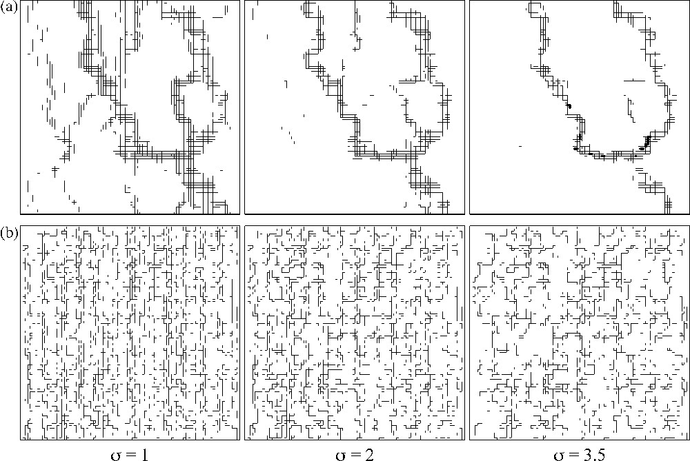
Comparison of the flow distribution. σ = Standard deviation of the lognormal distribution of bond conductivity. In light: bonds above the threshold of 1% of total inflow with a north–south-oriented general head gradient; in bold: bonds above the 30% threshold with both north–south- and east–west-oriented general head gradient. (a) The bond hydraulic conductivity is spatially correlated; (b) the bond hydraulic conductivity is uncorrelated in space.
Fig. 1. Comparaison de la distribution des flux. σ = Écart-type de la distribution log-normale des conductivités des liens. Les liens seuillés à 1 % pour un gradient de charge nord–sud sont représentés en noir, les liens seuillés à 30 % pour un gradient de charge nord–sud et est–ouest en gras. (a) Les conductivités hydrauliques des liens sont spatialement corrélées ; (b) les conductivités hydrauliques des liens ne sont pas spatialement corrélées.
Indexes quantifying the channelling effect for spatially correlated and uncorrelated bond conductivity. σ = Standard deviation of the lognormal distribution of bond conductivity. Flows are expressed in L3T−1
Tableau 1 Indices quantifiant les effets de chenalisation dans le cas où les conductivités des liens sont spatialement corrélées ou non. σ = Écart-type de la distribution log-normale des conductivités des liens. Les flux sont exprimés en L3T−1
| σ | 1 | 1.5 | 2 | 2.5 | 3 | 3.5 | |
| Correlated | Proportion of flow (%) in thresholded bonds | 78 | 86 | 91 | 93 | 95 | 96 |
| Proportion of bonds (%) thresholded at 1% | 22 | 18 | 15 | 13 | 11 | 10 | |
| Minimum bond flow [L3T−1] | 1 × 10−07 | 2 × 10−07 | 2 × 10−07 | 3 × 10−07 | 4 × 10−07 | 5 × 10−07 | |
| Maximum bond flow [L3T−1] | 3 × 10−06 | 6 × 10−06 | 1 × 10−05 | 2 × 10−05 | 3 × 10−05 | 4 × 10−05 | |
| Uncorrelated | Proportion of flow (%) in thresholded bonds | 74 | 81 | 86 | 88 | 90 | 92 |
| Proportion of bonds (%) thresholded at 1% | 30 | 29 | 28 | 26 | 25 | 24 | |
| Minimum bond flow [L3 −1] | 1 × 10−07 | 1 × 10−07 | 1 × 10−07 | 1 × 10−07 | 1 × 10−07 | 1 × 10−07 | |
| Maximum bond flow [L3T−1] | 9 × 10−07 | 1 × 10−06 | 2 × 10−06 | 2 × 10−06 | 3 × 10−06 | 3 × 10−06 |
Fig. 2 compares the evolution of the equivalent hydraulic conductivity Keq with the increase of the standard deviation for correlated and uncorrelated conductivity fields [11,28]. Keq is quite constant for uncorrelated conductivities, whereas it increases significantly (about three times between σ = 1 and σ = 3.5) when they are spatially correlated. In other words, a network made of a few highly conductive paths would be on average more permeable than a network with the same statistical distribution of local conductivity, but with evenly distributed flow paths [23]. Thus, getting an increased value of macroscopic conductivity compared with a theoretical mean calculated from the statistical distribution could also become an index of channelling. This index is interesting, since it does not need to ‘count’ flowing bonds or to calculate local flow rates. It can be calculated blindly, but requires however a prior guess on the statistical distribution of local conductivity values. Further work is needed to see whether this type of index is relevant and applicable in the field.
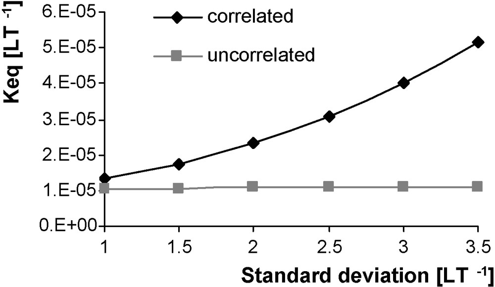
Comparison of the equivalent hydraulic conductivity for spatially correlated and uncorrelated bond conductivity.
Fig. 2. Comparaison de la conductivité équivalente du réseau de liens pour les cas corrélés et non corrélés.
Even if this type of evidence is not clearly reported at the scale of 3D fracture networks, one may suggest the existence of such nodes. The method proposed hereafter is first to distribute nodes over space; second to draw pipes between these nodes. Doing this gives the priority to a conditioning on node locations; additional prescribed conditioning on pipe features (length, orientation, etc.) will be used, but with possible bias in the generated network, since node locations are conditioned first. A few additional comments may argue in this sense:
- (1) nodes can be generated randomly but according to prescribed local densities (the number of nodes per unit volume). Of course, this node density is hardly available in field data, but it is expected intuitively, when fracture apertures are spatially correlated, that a densely fractured area will contain more nodes than a scarcely fractured one;
- (2) knowing that each flowing channel is included in a fracture plane, the orientation and the length of the channel are partly (indirectly) correlated with the dip, strike and length of the fracture. Thus, in a synthetic network, the pipe generation may inherit from information on the fracture field when available. However, conditioning is not to be followed strictly, which makes it reasonable that the conditioning of pipe features is partly biased when generating the network, since node locations are imposed first;
- (3) by fixing nodes first and then drawing pipes, the resulting network should be simpler, avoiding for instance dead ends and isolated non-flowing clusters. Further calculations are simplified and the network can be inverted on flow (and/or transport) measurements by making the hydraulic conductivity of the pipes vary, but also by deforming the network. This deformation can be performed by simply moving the node locations. On a numerical standpoint, the graph represented by the network does not change as well as the shape of matrices and vectors used to solve the discrete flow equations; this would obviously speed up the computations. We do not discussed hereafter on inversion capabilities of the networks, but this study is envisioned in the near future based on slug tests and interference pumping tests available from the Hydrogeological Experimental Site (HES) in Poitiers (France) [3,5,12,14].
Given the above general considerations, it is expected from the MODFRAC3D code presented hereafter that it is able to mimic the macroscopic hydraulic behaviour of a 3D fracture network by keeping only the channels where significant flow occurs. It must be pointed out however that even with a ‘strict’ conditioning, the simulated pipe network may be of a different geometry than the assumed real one. Actually, this feature is consistent with the philosophy of homogenisation inspiring this work: local geometry can be partly biased, provided that the global behaviour is respected.
3 Network generation and flow calculation
The generation of a network is initiated by means of a Poissonian spatial distribution to locate randomly the nodes, while honouring the constraint of volumetric node density in a cubic domain. The previous example of a fracture plane proved that nodes exist only if the distribution of local conductivities is spatially correlated. Then, for a given threshold on flux, the number of nodes increases with the standard deviation of the conductivity distribution and with the clustering effect separating in space highly conductive from almost impervious sub-areas. The consequence is that node density may vary in space and to allow this, a 3-D network can be divided into entities designated hereafter as sub-networks. A sub-network is spatially located in a parallelepiped volume defined by the min and max coordinates along the x, y and z directions: {xmin, xmax, ymin, ymax, zmin, zmax} and is characterised by its associated volumetric node density (or by a number of nodes).
Once the seeding of nodes in the parallelepiped volume of the sub-network according to the volumetric density is achieved, the next step is to draw pipes connecting these nodes. As stated above, a pipe is entirely located in a fracture plane. Thus, its orientation in space can be conditioned by the strike (direction of the steepest slope of the fracture plane) and dip (angle of this steepest slope with the horizontal plane) of the fracture plane. Moreover, the length, section, and conductivity of a pipe can also be correlated with the fracture aperture [27]. All this conditioning is achieved by associating a pipe with a family. A pipe family is defined by the statistical distribution of strike and dip of the fracture family to which it belongs and by the possible statistical distributions of pipe length, section, and conductivity. These distributions can be of three types: power law, lognormal, or negative exponential. Since pipes are grouped into families, it must be noted that a sub-network is also characterized by the percentages of each pipe-family that it may enclose. A sub-network may contain several ‘isolated’ clusters not connected with each other, but connected to the boundaries of the system (Fig. 3). Note also that isolated clusters of two different subnetworks may be connected between each other if specified in the input file, or if a vertical well is put in the system, establishing hydraulic connection between clusters of different subnetworks located at different depths.
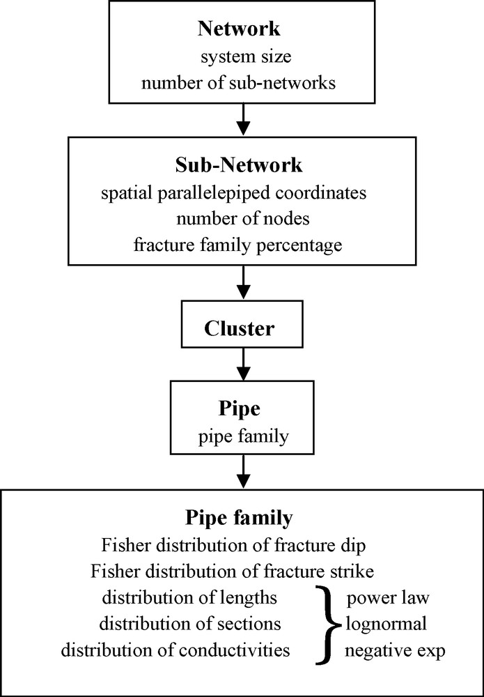
Hierarchy of the network (in bold: entities, in light: parameters).
Fig. 3. Hiérarchie du réseau (gras : entités, normal : paramètres).
Before describing the cluster generation (Fig. 3), we first focus on the generation of a single pipe. Two possibilities are available for the length of a pipe: either controlled by a power law, a lognormal, a negative exponential distribution or not controlled at all (not statistically constrained).
3.1 Pipe generation with a length obeying a statistical distribution
Knowing the location of a node (node #n), the program seeks another node (node #n + 1) to be connected with the first one by a pipe (Fig. 4). A pipe family is selected randomly according to its chosen proportion (or probability) among the available families. A dip θ and strike ϕ are also drawn from the corresponding statistical distributions. Moreover, a length l is randomly selected in the corresponding length distribution of the family. A ‘virtual’ plane P of dip θ and strike ϕ and passing by node #n is then drawn. On P, a ‘virtual’ circle C is drawn centred on node #n and of radius l. At node #n, the straight line (D) laying on P and perpendicular to the projection of the global head gradient divides C into two semicircles C+ and C−. They correspond to the positive and negative directions with respect to the global head gradient, respectively. According to a prescribed direction, e.g. along C−, the algorithm seeks the node closest to C− and located in a prism of axis (D) and angle α, a specified tolerance parameter. The prism allows us to look for a node #n + 1 yielding a pipe [#n–#n + 1] with a few fluctuations on length strike and dip around the prescribed values. Otherwise, it is very unlikely to find a node #n + 1 giving a pipe able to match up strictly the prescribed values. If a node (#n + 1) is found, the pipe is generated. If no node is found on C, other attempts can be done from node #n after redraw of the pipe length. If the third attempt fails in seeking node #n + 1, the pipe is automatically generated as the line passing by node #n and intersecting the boundary of the system along the direction parallel to the global head gradient. Of course, generating a pipe in this latter case will partly bias the possible prescribed pipe length distribution. But it must be reminded that the priority is to honour first the node locations with the aim to generate a channel network as simple as possible, without dead ends and for which nodes could then be moved for inversion purpose (see Section 2). Note also that the risk to generate by default a pipe intersecting the boundary is lowered when the density of nodes is high and when the search angle α (see above) is well chosen (the weaker the node density, the larger the angle).
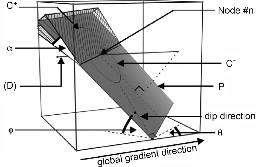
Search procedure in the generation of a pipe.
Fig. 4. Procédure de recherche lors de la génération d’un tube.
3.2 Pipe generation with uncontrolled length
In this case, instead of seeking the node closest to the semicircle (C+ or C−), the algorithm looks for the node closest to node #n and located in the same prism of axis (D) and angle α (Fig. 4) The interest of uncontrolled length is to keep precision on the dip and strike distributions that may be partly biased by the generation of a pipe with prescribed length (see above). Note that a lack of information in the field on the size of fractures and/or channels may also justify the generation of pipes with uncontrolled lengths.
3.3 Cluster generation
Since the generation process is the same for each subnetwork, for the sake of simplicity, only a single sub-network will be considered below. A node is selected randomly among all the nodes belonging to the subnetwork (node #0, Fig. 5). The algorithm consists in generating two ‘half-clusters’ from node #0 and connecting the upper constant head boundary (nodes are sought in the positive direction, see above) and the lower head boundary (nodes are sought in the negative direction). The generation of the first half-cluster begins with the generation of the first bond in the negative direction connected to node #0 (see above for the conditioning–unconditioning of the pipe length). After node #1 (i.e. the tip of the first pipe) has been found, the algorithm is then iterated from node #1 until the half-cluster is connected to the lower constant head limit (nodes #0, #1, #2, Fig. 5). The second half-cluster starting at node #0 is generated in the same way, but in the positive direction (nodes #0, #3, #4, Fig. 5). Finally, the two half-clusters form the entire first cluster. The next cluster is built in the same way. A node is selected randomly among the remaining available free nodes, i.e. the nodes that do not belong to the previous cluster (e.g., node #12, Fig. 5), and a new cluster is generated according to the previous algorithm. However, the generation of a half-cluster stops either when it intersects the boundary of the block (node #14 in the positive direction), or when it intersects a node belonging to a previous cluster (node #5). In the latter case, this yields to the connection of the two clusters. The cluster generation is iterated until there are no longer available free nodes. Note that a node shared between several clusters cannot be connected to more than six nodes, potentially: four pipes representing the four channels of two intersecting fractures and two pipes for the fracture intersection [22].
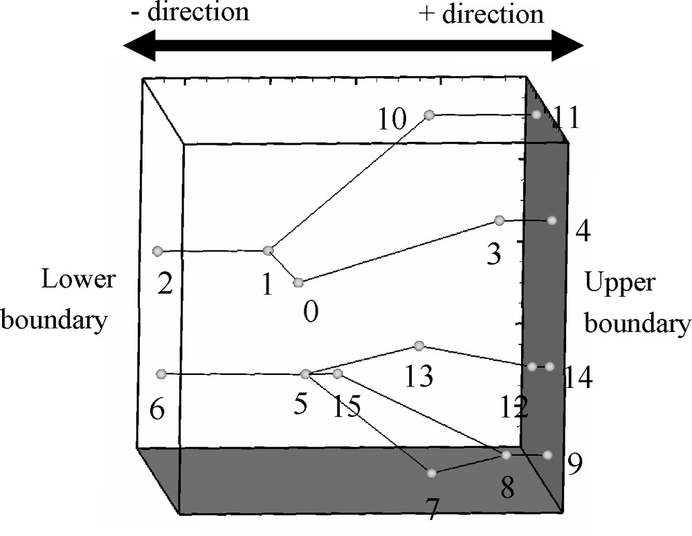
Cluster generation (the numbers correspond to the generation order).
Fig. 5. Génération d’un amas (les numéros correspondent à l’ordre de génération).
3.4 Boreholes
Boreholes can be introduced in the model by specifying for each of them their location, the subnetworks they intersect, and the location of intersecting nodes, and the prescribed pumping/injection flow rate. The value of the hydraulic conductivity assigned to a pipe representing a borehole is much higher than the pipe's conductivity, so that the hydraulic head calculated along the borehole is almost constant. Note that the flow rate prescribed at the borehole can also be cancelled out. In that case, the borehole merely plays the role of a bond of high hydraulic conductivity, which connects two different subnetworks.
3.5 Flow calculation
Remember that the rock matrix is assumed impervious and flow in the confined system only occurs in open pipes, with the consequence that all the open volume is occupied by the fluid. The domain is a 3D cubic block of size L × L × L, with ‘permeameter-type’ boundary conditions: constant prescribed head at two opposite faces and no flow at the four others. The direction of the general head gradient can be set by the user (i.e. the choice of the two faces assigned with a constant head), meaning that only three gradient directions are available. Each cylindrical pipe between two nodes is of constant diameter and thus constant hydraulic conductivity along its length, but both parameters may vary from pipe to pipe. Diameter (or section) and conductivity can be correlated (stating that a diameter implies a conductivity) or not.
A pipe is considered as continuous, homogeneous and the flow is supposed to be laminar, so that Darcy's law remains applicable. A finite volume approach associated with Kirchhoff's law (mass balance principle at each node) is used to calculate the hydraulic head for both transient and steady-state conditions. In steady-state flow, it is simply stated that the total inflow and outflow at each node are equal. In transient flow conditions, the storage capacity of a node is associated with half of the volume of its attached pipes, and the accumulation term of the local flow equation (including a composite compressibility between water and rock matrix) applies over this half volume. Note that this assumption is necessary to calculate a correct mass balance in discrete equations. Both in steady-state and transient conditions, the discrete equations (with an implicit scheme as regards the time variable for the transient case) yield an n × n linear system with a symmetric positive definite matrix. The latter is sparse and a so-called ‘compressed row storage method’ is used to store only the non-zero terms and thus save memory space. The solver used to compute the heads is a compressed matrix preconditioned conjugate gradient algorithm.
4 An example
The code is asked to mimic a fully known ‘synthetic’ network made up of four fractures generated by the code FRACMAN [15] (Fig. 6a). The space is discretized in 100 × 100 × 100 square meshes. Each fracture plane is characterized by a spatially correlated hydraulic conductivity (with a spherical variogram of range the half-length of the fracture plane) following a lognormal distribution (μ = –5, σ = 1 in decimal log). As shown in Section 2, correlation + highly variable values of conductivity are assumed to yield channelled flow with invariant ‘crux nodes’.
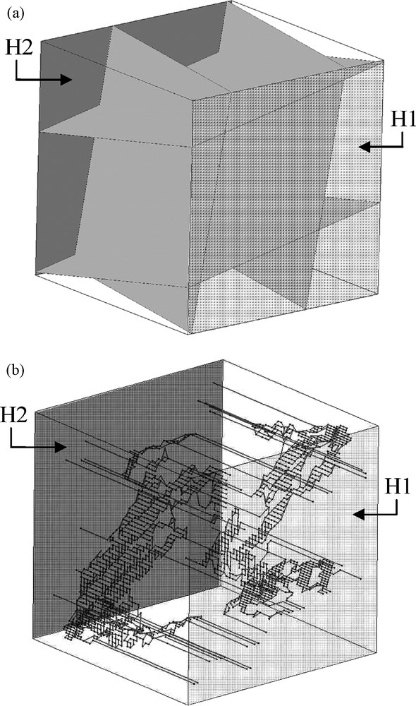
(a) Network of four fractures generated by FRACMAN. (b) Channel network generated by MODFRAC3D.
Fig. 6. (a) Réseau de quatre fractures généré avec le code FRACMAN. (b) Réseau de chenaux généré par MODFRAC3D.
‘Permeameter-type’ conditions are applied at the boundary and the flow is then computed for the three possible gradient directions (along the three principal directions of the block). A threshold is then applied as follows: meshes in which flow is higher than 1.5‰ of the total inflow for the three gradient directions are marked, and they will represent the location of the crux nodes for the pipe network generated with MODFRAC3D (black points, Fig. 6b). For a given gradient direction, the aim is to generate a pipe network that best mimics the behaviour of the reference four fractures. The latter are separated into two families (two fractures in each family) of identical dip and strike. The length of the pipes is not controlled, since there are not enough nodes to get a significant representation of any prescribed pipe length distribution. This information as well as the location of the crux nodes is given to MODFRAC3D. As shown in Fig. 6b, the simulator generates the equivalent channelled flow field with a very small number of pipes and one just needs to set the local product KS (conductivity × section) of each pipe at 9.63 × 10⁻³ [L3T−1] to obtain a similar equivalent hydraulic conductivity.
The two networks are then compared in terms of channelling effect by comparing local flux distributions. For the set of four fractures and the given gradient direction, the meshes that have a flow higher than 1.5‰ of the total inflow are kept and assumed to represent the reference channel network. Since ‘crux nodes’ of the pipe network are also determined with the same threshold but for the three gradient directions, they are included in the reference network of channels. Fig. 7 displays the flow distribution for both the reference network of channels extracted from the four fractures and the pipe network generated by MODFRAC3D. The correlation between both distributions is good, the correlation coefficient is 0.97, and the relative errors on mean and variance between both distributions do not exceed 13%. Finally, the pipe network generated by MODFRAC3D has the same equivalent hydraulic conductivity and almost the same flux distribution. One may therefore consider that this pipe network is a good representation of channelled flow in fractures. Of course, the local geometry is not preserved, since the pipe network is a ‘homogenised’ and much simpler image of the real channel network. Nevertheless, this facilitates further modelling exercises and computations.
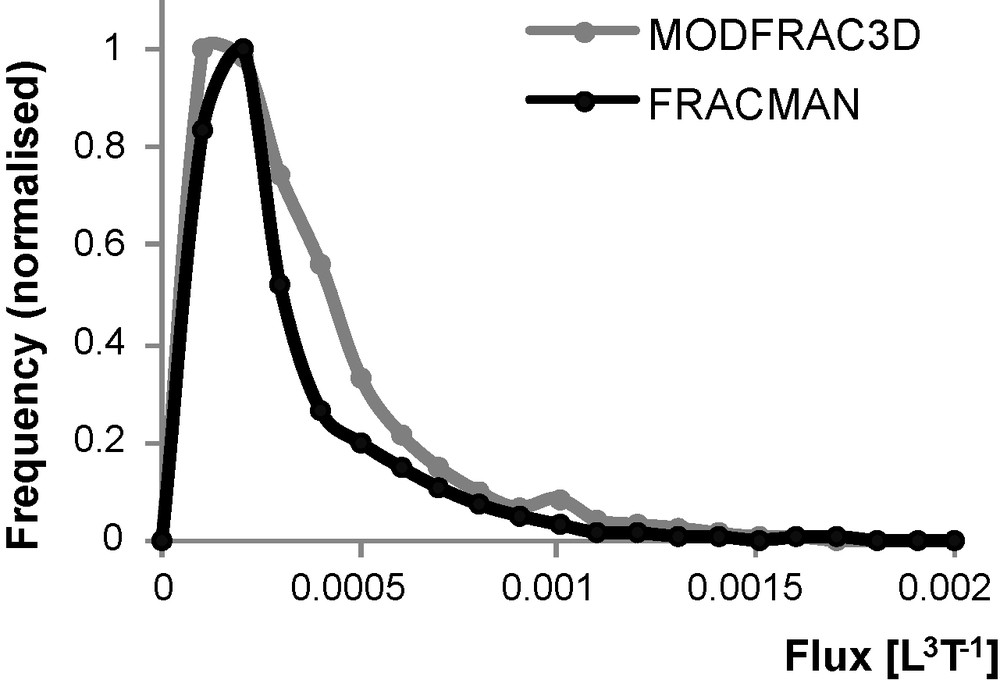
Distribution of flux in the FRACMAN network thresholded at 1.5‰ of the total inflow and in the MODFRAC3D pipe network.
Fig. 7. Distribution des flux dans le réseau généré par FRACMAN seuillé à 1,5 ‰ du flux total et dans le réseau de tubes généré par MODFRAC3D.
5 Conclusion
This work is a first approach to flow and transport in fractured rocks for which the principal conditioning is based on general considerations stating that (i) flow is highly channelled both in each fracture plane and at the scale of the entire fracture network; (ii) there exist some invariant crux nodes through which flow must pass whatever the general flow direction.
The features mentioned above have motivated a new method to build a discrete fracture network. Usually, planar objects (or bonds) are ‘dropped’ in a Euclidean space and intersections of objects are the consequence of the dropping. In the present case, crux nodes are dropped first according to a varying or uniform density in space, and then, bonds are generated between these nodes to build a channel network. Length and orientation of bonds can be conditioned on statistical distributions, but the latter may be slightly biased on the final network, since node locations are honoured first. The bias is a priori all the more important if the node density is small.
In the end, the channel network assumed to represent the major flow paths in a fracture field (or a rough fracture plane) is quite simple in terms of topology; for instance, it does not enclose dead ends and the number of bonds is small. This should facilitate further flow and transport computations. Because of this simplicity, it can be envisioned to inverse flow and transport measurements by making the properties of bonds to vary, but also by deforming the network by moving the node locations. This deformation would not change the topology of the graph representing the network, thus the shape of the matrices of the linear systems to solve the flow (and transport) equations would remain unchanged. Of course, this would speed up the inversion in simplifying computations at each convergence iteration.
Vous devez vous connecter pour continuer.
S'authentifier