Identification of aquifer point sources and partial boundary condition from partial overspecified boundary data

Najla Tlatli Hariga; Rachida Bouhlila; Amel Ben Abda

doi:10.1016/j.crte.2007.11.006

Résumés

Anglais
Français

In this work, we present a new mathematical method that allows recovering of the wells fluxes and hydraulic heads on a part of the boundary where they are not known, for an aquifer domain having overspecified boundary data on another part of its boundary. The method is based on the minimisation of an energy-like error functional of Andrieux and Ben Abda [Inverse Probl. 22 (2006) 115–133] for the missing-data recovering step and on the Reciprocity Gap principle of the same authors [Inverse Probl. 12 (1996) 553–564] for point sources identification.

Nous nous proposons dans ce travail de résoudre un problème de Cauchy, afin de retrouver les débits des puits et la condition de charges imposées sur une partie de la frontière d’un aquifère, à partir de données partielles surabondantes sur une autre partie de la frontière. La résolution se fait en deux étapes : on commence par minimiser la fonctionnelle d’erreur d’énergie développée par Andrieux et Ben Abda [Inverse Probl. 22 (2006) 115–133] pour compléter les données, puis on applique le principe de réciprocité introduit par les mêmes auteurs [Inverse Probl. 12 (1996) 553–564] pour déterminer les débits.

1 Introduction

The leading inverse problem in hydrogeology deals with estimating the hydrodynamical parameters of the aquifer: permeabilities, transmissivities, and storage coefficients. The most frequent problem and also the most studied in the literature is indeed that of the determination of transmissivities from piezometric data in a steady-state flow regime [9,10]. However, in many real situations, uncertainties can be related to the aquifer domain itself, its boundary conditions and also, usually, on the external constraints, such as withdrawal rates in wells, drillings, and recharge.

The knowledge of the aquifer withdrawal rates can represent a largely unknown factor in real problems of groundwater resources modelling. The acquisition of these data is expensive and prone to great uncertainties. The usual techniques of specific measurements or estimation, using, e.g., surveys of power consumption or crop surfaces, type and degree of growth of the irrigated crops and also satellite images, provide only orders of magnitude. Indeed, usually, this term of external forcing constitutes data to be refined in a global model calibration procedure.

The problem under consideration can be stated mathematically as the recovery of unknown heads on a part of the domain boundary and of the prescribed flux for known point sources from Cauchy data. The identification procedure relies on two steps:

• the recovery of the missing boundary data, which is reduced to solving the Cauchy problem;
• the identification of the well fluxes.

The first step is the most difficult one, because, since Hadamard [8], the Cauchy problem is known to be severely ill posed. The most popular method known in the hydrogeology community, as reported in the review papers [9,10], consists, roughly speaking, in drawing the flow streamlines. Even though this method is easy to implement, it is very sensitive to measurement errors. It is therefore usually exploited together with a regularizing procedure [4].

Our approach in solving the Cauchy problem is borrowed to the solid mechanics community: it relies on a method of minimizing a misfit energy-like function. We adapt this energy-like error to the Darcy framework.

2 The model

We will focus, in this note, on extending the data completion algorithm based on an energy error functional, initially introduced for the Laplace equation [3] to the Darcy framework [5]. The potential application concerns the identification of well extraction in an aquifer with known transmissivities and prescribed piezometric levels on a part of its boundary, in steady-state conditions.

Using the notations shown in Fig. 1, a simplified mathematical model is given by:

\{\begin{array}{l} - Div (Tgrad (h)) = \sum_{k} Q_{k} δ_{s k} in Ω \\ h = H on Γ_{m} \\ T \frac{\partial h}{\partial n} = ϕ on Γ_{m} \end{array}

(1)

where T is the transmissivity, which can be a scalar if the medium is isotropic and homogenous, or a function in case of heterogeneity, or a second-order tensor for the anisotropic case. The hydraulic head is denoted by h, Q_k is the well abstraction, corresponding to a point source located at S_k with coordinates (x_k,y_k), and δ is the Dirac distribution. Γ_m is the portion of the boundary of Ω where both h and its normal derivative are known (i.e. an overspecified condition) and Γ_u is the part of the boundary where all information is lacking. This situation can correspond to an arbitrary boundary for an aquifer known to extend over Γ_u, but where no information is available. It is for example the case of a deep aquifer continuing beyond the shoreline below the sea bottom. Indeed, from a practical viewpoint, as the known piezometric levels correspond to measured values in boreholes and are presented as interpolated isolines, it is easy to calculate their normal derivative, even on an internal part of the domain, but close to the boundary isopiezometric line, in order to obtain the overspecified data. We propose, in this paper, to reconstruct the missing data using an energy-like error functional introduced in [3] and then to determine the point source fluxes via the reciprocity gap principle [1,2,6].

Fig. 1
The mathematical domain with wells.
Fig. 1. Domaine du modèle mathématique avec les différents puits.

3 Mathematical identification process

3.1 Data completion

Let us consider the above Cauchy problem (equation 1). Provided the data H are compatible with the flux ϕ, the data completion step is achieved in a neighbourhood of the boundary of the domain where there is no well. A fictitious inner boundary Γ_F is therefore introduced. Then the energy-like error functional is constructed on the fictitious domain Ω_F with ∂Ω_F = Γ_m ∪ Γ_u ∪ Γ_F and Γ_H ₌ Γ_u ∪ Γ_F. Extending the data means finding (ϕ,f) such that we obtain equation. (2):

\{\begin{array}{l} - Div (Tgrad (h)) = 0 in Ω_{F} \\ h = H, T \frac{\partial h}{\partial n} = ϕ on Γ_{m} \\ h = f, T \frac{\partial h}{\partial n} = φ on Γ_{H} \end{array}

(2)

The approach in the energy-like error functional method developed in [3] follows two steps. First, we consider, for a given pair (η,τ), the two following mixed well-posed problems (equations (3a) and (3b)):

\{\begin{cases} - Div (Tgrad (h_{1})) = 0 in Ω_{F} \\ h_{1} = H on Γ_{m} \\ T \frac{\partial h_{1}}{\partial n} = η on Γ_{H} \end{cases}

(3a)

\{\begin{cases} - Div (Tgrad (h_{2})) = 0 in Ω_{F} \\ h_{2} = τ_{o n} Γ H \\ T \frac{\partial h_{2}}{\partial n} = ϕ on Γ_{m} \end{cases}

(3b)

The second step is to build an energy-like error functional on the pair (η,τ), using an energy norm, denoted E. Indeed, these fields are obviously equal only when the pair (η,τ) meets the real data (ϕ,f) on the boundary Γ_H = Γ_u ∪ Γ_F. We propose then to solve the data completion problem via the following minimization algorithm (equation (4)):

(φ, f) = \arg \min E (η, τ)

(4)

E (η, τ) = \frac{1}{2} \int_{Ω_{F}} {(T grad (h_{1}) - T grad (h_{2}))}^{2} d Ω

(5)

3.2 The reciprocity gap principle

After the first step of reconstructing the missing boundary data, we deal with recovering the unknown well fluxes via the Reciprocity Gap functional. This functional has been introduced in [2] in the context of planar cracks identification from overspecified boundary data. It relies on the well-known Mawell–Betti reciprocity principle. As introduced in [2], it relates the overdetermined boundary data to the unknown quantities (here the well fluxes).

We multiply the first equation of the system (1) by a virtual field $v$ satisfying Div(gradμ) = 0, then we integrate it over the whole domain Ω; we use Green's second formula, we find:

R (v) = \sum_{k} Q_{k} v (S_{k})

(6)

where

R (v) = \int_{\partial Ω} T (\frac{\partial h}{\partial n} v - \frac{\partial v}{\partial n} h) d Γ

(7)

Notice that the left-hand side of the equality (6) or (7) is totally known: (ϕ, H) are the overdetermined boundary data and we can select v.

More precisely, for k wells with unknown fluxes, we evaluate R(z^j), where z is the complex variable, such that the real and imaginary parts of z^j are harmonic:

R (z^{j}) = \sum_{k} Q_{k} z_{k}^{j}

(8)

where z_k = x_k + i y_k is the affix of the point source S_k.

Then we exploit the reciprocity gap functional with various particular fields μ.

Therefore, the determination of the fluxes of a collection of wells amounts to solving a linear system:

A Q = b

(9)

where

A = (z_{j}^{i})

is the Wandermonde matrix, Q = (Q_j) and b = (R(zⁱ)).

To clarify this step, we carry out an example in the case of two wells located at the points M₁(x₁,y₁) and M₂(x₂,y₂) with fluxes Q₁ and Q₂. The particular harmonic $v$ chosen are:

v_{1} = 1 \nabla v_{1} n = 0

v_{2} = x + i y \nabla v_{2} n = 1 + i

Then we apply equations (6) and (7) for each

v

\begin{array}{l} R (v_{1}) = \sum_{k} Q_{k} v_{1} (S_{k}) = Q_{1} + Q_{2} = \int_{\partial Ω} T \frac{\partial h}{\partial n} d Γ \\ R (v_{2}) = \sum_{k} Q_{k} v_{2} (S_{k}) = Q_{1} (x_{1} + i y_{1}) + Q_{2} (x_{2} + i y_{2}) \\ R (v_{2}) = \int_{\partial Ω} T \frac{\partial h}{\partial n} (x + i y) - T h (n_{x} + i n_{y}) d Γ \end{array}

Finally, we have to solve one of the equivalent linear systems, corresponding to the real and imaginary parts of system (8), with k = 2:

[\begin{array}{c} Q_{1} & Q_{2} \end{array}] = [\begin{array}{c} 1 & x_{1} \\ 1 & x_{2} \end{array}] = [\begin{array}{c} \int_{\partial Ω} T \frac{\partial h}{\partial n} d Γ & \int_{\partial Ω} T (\frac{\partial h}{\partial n} x - h n_{x}) d Γ \end{array}]

[\begin{array}{c} Q_{1} & Q_{2} \end{array}] [\begin{array}{c} 1 & y_{1} \\ 1 & y_{2} \end{array}] = [\begin{array}{c} \int_{\partial Ω} T \frac{\partial h}{\partial n} d Γ & \int_{\partial Ω} T (\frac{\partial h}{\partial n} y - h n_{y}) d Γ \end{array}]

so that we obtain directly Q₁ and Q_2.

4 Numerical trials

The resolution of the problem given by equation (2) was carried out using the finite-element method (FEM). First, we complete the boundary data via an optimisation problem, then we determine the wells fluxes via the resolution of a linear problem.

For minimizing the energy functional E (equation (4)), we have to compute the gradient of E with respect to all the components of the unknown field h (here equal to the number of nodes of the mesh). Therefore, we have chosen the adjoint state method because it does not depend on the number of components, and it makes it possible to evaluate the gradient in any direction using only the determination of two adjoint fields.

All the computations have been run on FemLab [7].

The numerical tests are performed on the following geometry (Fig. 2), corresponding to a rectangular domain of 20 km × 10 km, with a homogeneous transmissivity T = 0.001 m² s⁻¹ with overspecified data on the upper side and missing data on the lower one. The overspecified data are extracted from the exact solution h(x,y) of the direct problem given by equation (1) with point sources coordinates (x_k,y_k) and intensity Q_k:

h (x, y) = \sum_{k} \frac{Q_{k}}{2 π T} log (\sqrt{{(x - x_{k})}^{2} + {(y - y_{k})}^{2}})

(10)

The domain is meshed with a regular mesh of triangular elements with linear interpolation, characterized by 1100 nodes and 348 elements. To test the efficiency of the proposed reconstruction processes, different cases have been studied.

Fig. 2
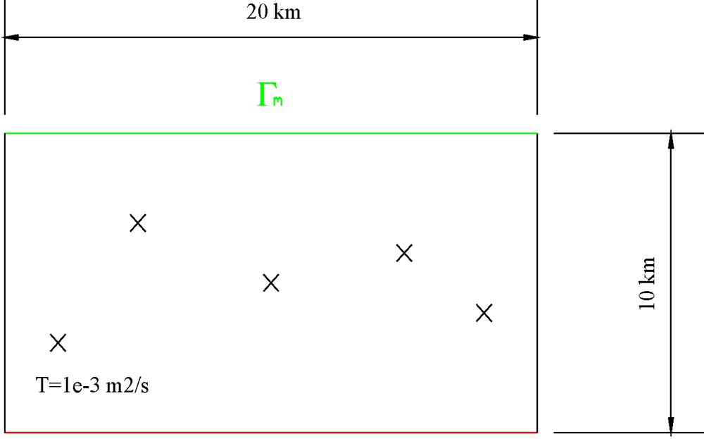
The studied domain with the five wells.
Fig. 2. Domaine étudié avec cinq puits.

4.1 The case of multiple wells

We consider in this case a collection of five wells with positive and negative fluxes. Well locations and fluxes are shown in Table 1, whereas Table 2 sums up the calculated fluxes and the relative errors compared to the exact values. These last values correspond to the exact solution of the forward problem given by equation (10). On Tables 3 and 4, we consider the same five wells with fluxes values 10 and 100 times less than those of Table 2. As the piezometric levels are linear with respect to the fluxes (as shown in equation (10)), the error remains almost identical for the three cases.

X (km)	2	5	10	15	18
Y (km)	3	7	5	6	4
Q_k (l s⁻¹)	−50	−70	150	−30	80

Q_{k exact} (l s⁻¹)	−50	−70	150	−30	80
Q_{k calc.} (l s⁻¹)	−57	−68.1	152.1	−33.3	85.1
Relative error (%)	14	2.7	1.4	11	6.25

Q_{k exact} (l s⁻¹)	−5	−7	15	−3	8
Q_{k calc.} (l s⁻¹)	−5.7	−6.8	15.2	−3.3	8.5
Relative error (%)	14	2.8	1.3	10	6.25

Q_{k exact} (l s⁻¹)	−0.5	−0.7	1.5	−0.3	0.8
Q_{k calc.} (l s⁻¹)	−0.57	−0.68	1.52	−0.33	0.85
Relative error (%)	14	2.8	1.3	10	6.25

Fig. 3a shows the reconstructed data (the hydraulic head and its normal derivative) over the boundary where data are missing, the lower one, in the case of these five wells. Fig. 3b represents the hydraulic head over the entire domain in the case of five wells. We note that the completion results match very well the exact ones.

Fig. 3
(a) Hydraulic head and its normal derivative over Γ_u; (b) isovalue of the hydraulic head in the case of five wells.
Fig. 3. (a) Charge hydraulique et sa dérivée normale sur Γ_u ; (b) isovaleur de la charge hydraulique, dans le cas de cinq puits.

4.2 Sensitivity to noisy data

To take into account the sensitivity of the recovered well fluxes to noisy data, a uniform white noise (with zero mean), is applied to the Dirichlet data on Γ_m in the case of a single well located at x = 2 km and y = 5 km, with a rate Q = −100 l s⁻¹. Table 5 shows the errors for a noise level up to 8%. One can see that, despite the noise, the data recovering error remains acceptable, for a noise level less then 6%.

Noise level (%)	0	2	4	8
Relative error (%)	0.3	3	4	6

4.3 Sensitivity to the relative position

In the third case, we test the sensitivity to the relative position of two wells. We consider two wells with fluxes: Q₁ = –100 l s⁻¹ and Q₂ = −50 l s⁻¹, separated by a variable distance d, and we compute the relative error on recovered fluxes for each distance (see Table 6). One can observe that if the wells are well separated (far from each other), the fluxes are well identified, but when the distance between the wells decreases, the identification procedure is less accurate.

Distance d (km)	16	10	6	3	2	1.5
Relative error (%)	2	6	8	9	15	17

5 Conclusion

The presented identification procedure of aquifer point sources from partially overspecified boundary data appears satisfactory in all the tested cases: multiplicity of wells, noisy data, and relative position of wells.

In the general context of aquifer modelling, this point sources’ identification procedure could be carried out, for each transmissivity field identification by whatever inverse method, as well as iterations between the two identification problems, transmissivities on the one hand, and well fluxes and partially unknown boundary conditions on the other one.

A natural extension of this work will deal with heterogeneous domains (for hydrodynamical properties) and real aquifer data.

Acknowledgements

This work was supported by the ‘Ministère de la Recherche scientifique, de la Technologie et du Développement des compétences (MRSTDC, Tunisia) under the LAB-STI-02 and LAB-ST-03 Program and, partially, by the Hydro3 + 3 M06/02 (Numerical Computing Groundwater Flows) and the ‘Fonds national pour la recherche scientifique’, Switzerland (JRP Project Gestion durable des ressources en eaux souterraines côtières. Modélisation physique et probabiliste. Application à la côte orientale du cap Bon, Tunisie).