

1 Introduction
In two decades, the connection between solar activity and the Earth's atmosphere has moved from a mere curiosity to a hotly debated topic. Many reviews have been written, emphasising either the radiative forcing from a solar viewpoint (Foukal et al., 2006; Fröhlich and Lean, 2004; Lean, 1997; Lean, 2005; Lean and Rind, 1998) or from a terrestrial viewpoint (Haigh, 2005; Haigh, 2007), solar variability in general (Alley et al., 2007; Benestad, 2006; Calisesi et al., 2007; Friis-Christensen et al., 2000; Lockwood, 2005; Pap et al., 2004; Rind, 2002), historical aspects and long-term effects (Bard and Frank, 2006; Beer et al., 2006; de Jager, 2005; Hoyt and Schatten, 1997; Usoskin, 2008; Versteegh, 2005), and other, indirect mechanisms (Marsh and Svensmark, 2003; Tinsley, 2008). Here, we review the solar inputs to the terrestrial atmosphere and focus on their origin, the underlying physics and their observation.
The Sun–Earth connection is a world of paradoxes. Until recently, this seamless system was widely considered as a stack of independent layers, and only in recent times did the interactions between these layers really attract attention. The role of the Sun in our solar system goes undisputed, and yet the effect of solar variability on the atmosphere remains quite controversial. As we shall see later, the main mechanisms by which the Sun affects the Earth are not the most immediate ones in terms of energetic criteria.
The Sun – like any living star – continuously radiates energy outward into the heliosphere. The radiated energy is carried by:
- • electromagnetic waves over a frequency band ranging from radio waves to hard X-rays;
- • a stream of hot plasma (the solar wind) consisting primarily of electrons and protons with a small fraction of heavier ions;
- • an interplanetary magnetic field (IMF) which is carried along with the solar wind (often referred to as a frozen-in magnetic field);
- • violent solar outbreaks such as solar flares and coronal mass ejections (CME) (Kamide and Chian, 2007).
The solar radiative output is nearly constant in time and accounts for about 1365 W/m2 at a solar distance of 1 Astronomical Unit (AU), with a solar cycle dependent variation of the order of 0.1%. Under quiet solar conditions, the flow rates of the kinetic energy of the solar wind bulk motion and the solar wind thermal energy amount to about 5 × 10⁻⁴ W/m2 each at 1 AU, i.e., a million times less than the radiative input. The energy flow rate of the IMF is another two orders of magnitude smaller, about 5 × 10⁻⁶ W/m2. Yet, these different mechanisms all have a distinct impact on the terrestrial atmosphere and none of them can be ruled out, a priori.
Nearly 70% of the solar radiation that arrives at the top of the Earth's atmosphere is absorbed in the atmosphere or at the Earth's surface; the rest is immediately reflected. In contrast, the efficiency of energy transfer from the solar wind into the magnetosphere is only 1–10%, depending on the orientation of the IMF.
Wave and particle emissions are not the only means by which the Sun can influence the Earth's atmosphere. The solar wind plasma, more precisely, the IMF associated with it, modifies the rate of penetration of interstellar energetic particles into the heliosphere and eventually into the atmosphere. This has led to one of the more controversial aspects of Sun–climate studies.
In this review, we first start with an illustration of solar variability on time scales from days to decades (Section 2). Section 3 then addresses the solar radiative output and its effects, and Section 4 the role of orbital changes. Thereafter, we focus on indirect effects, the electric circuit (Section 5, including galactic cosmic rays [GCR]), atmospheric convection under quiet (Section 6) and active (Section 7) solar conditions, and the role of the coupling with upper atmospheric layers (Section 8). Conclusions follow in Section 9. External forcings that are not related to the Sun (such as volcanic activity) and internal forcings are not addressed.
2 Solar variability
Solar activity affects the Earth's environment on time scales of minutes to millions of years. The shorter time scales are of particular interest in the frame of space weather1 (Schwenn, 2006), but will not as much be considered here. Long-term changes of solar and heliospheric conditions and their manifestation in the Earth's space and atmospheric environment are typically considered to be in the realm of space climate (Mursula et al., 2007). It is often believed that only slow variations (i.e. time scales of years and above) can affect climate. This is not fully correct in the sense that the rate of occurrence of fast transients such as solar flares is modulated in time, so that all time scales eventually matter.
To give a glimpse on the complexity of solar variability, we illustrate in Fig. 1 the variation of some key solar-terrestrial parameters; several of them will be discussed in later sections. The long time interval (left panel) covers 3 decades only because very few accurate solar observations were available before the advent of the space age. One of the main tasks in solar-terrestrial physics today is to extrapolate these tracers backward in time.
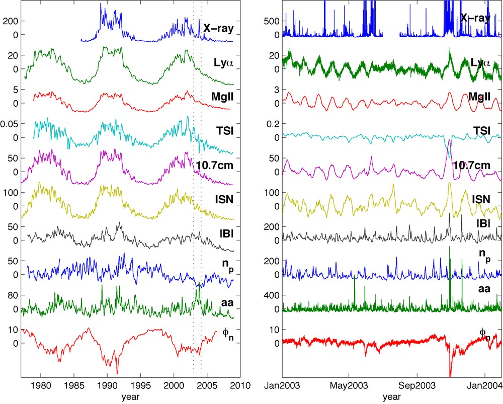
Relative variation (in percentage) of some of the key solar-terrestrial parameters. The left plots shows 3 decades of observations, with monthly averaged data and the right plot a 1-year excerpt with hourly or daily observations. From top to bottom: soft X-ray flux (from GOES/SEM), irradiance in the EUV (Lyman-α line composite from LASP, Boulder), irradiance in the UV (MgII index from NOAA), Total Solar Irradiance (TSI composite from PMOD-WRC, Davos), radio flux at 10.7 cm (from Penticton Observatory), sunspot number (ISN, from SIDC, Brussels), intensity of the magnetic field in the solar wind (|B|, from OMNIWeb), proton density in the solar wind (np, from OMNIWeb), aa geomagnetic index (from ISGI, Paris) and neutron flux at mid-latitude (ϕn, from SPIDR). All quantities are normalised with respect to their time-average. Some of the vertical scales differ between the two plots.
Fig. 1. Variation relative (en pourcentage) de quelques paramètres-clé des relations Soleil–Terre. La figure de gauche montre trois décennies d’observations, avec des moyennes hebdomadaires ; celle de droite couvre une année d’observations, avec des moyennes journalières ou horaires. De haut en bas : le flux de rayons X mous (de GOES/SEM), l’irradiance dans l’EUV (composite de la raie Lyman-α ; LASP, Boulder), l’irradiance dans l’UV (indice MgII ; NOAA), l’irradiance solaire totale (composite de la TSI ; PMOD-WRC, Davos), flux radio à 10,7 cm (Observatoire de Penticton), nombre de taches solaires (ISN ; SIDC, Bruxelles), intensité du champ magnétique dans le vent solaire (|B| ; OMNIWeb), densité de protons dans le vent solaire (np ; OMNIWeb), indice géomagnétique aa (ISGI, Paris) et flux de neutrons à moyenne latitude (ϕn ; SPIDR). Toutes les quantités ont été normalisées par rapport à leur moyenne temporelle. Certaines échelles verticales peuvent différer entre les deux graphes.
The tracers (or proxies, as they are usually called) of solar activity that are shown in Fig. 1 are respectively:
- • X-ray: the soft X-ray flux between 0.1 and 0.8 nm, which is indicative of the energy released during solar eruptive phenomena such as flares. Most of this radiation is absorbed in the upper atmosphere (above 60 km) and above;
- • Lyα: the intensity of the bright H Lyman-α line at 121.57 nm, which is mainly emitted in the solar transition region and is absorbed in the ionosphere (above 90 km);
- • MgII: the core-to-wing ratio of the Mg II line at 279.9 nm, which is a good proxy for the solar irradiance in the ultraviolet (UV). This radiation is primarily absorbed in the stratosphere, where it affects ozone concentration;
- • TSI: the Total Solar Irradiance (TSI), which represents the total radiated power measured at 1 AU, above the atmosphere. This quantity summarises the total radiative energy input to the Earth;
- • 10.7 cm: the radio flux emitted at 10.7 cm, or decimetric index. This radiation has no direct impact on climate, but it is widely used in Global Circulation Models (GCM) as a proxy for solar activity. It is measured daily since 1947;
- • ISN: the International Sunspot Number (ISN), one of the most ancient gauges of solar activity, with almost daily measurements since 1749;
- • |B|: the intensity of the IMF at the L1 Lagrange point, just upstream of the Earth;
- • np: the proton density, also measured in the solar wind. This quantity, combined with the solar wind bulk speed, gives the solar wind dynamic pressure, which is the main solar parameter to define the shape of the magnetosphere;
- • aa: the aa-index, which is a 3-hourly range measure of the level of geomagnetic field fluctuations at mid-latitudes. Its amplitude reflects the amount of magnetic energy that is released in the terrestrial environment;
- • ϕn: the atmospheric neutron flux, measured on Earth, at mid-latitude. This flux is indicative of the highly energetic galactic cosmic ray flux, which is not of solar origin, but is modulated by solar activity. Part of this ionising radiation is absorbed in the middle atmosphere, where it might affect cloud condensation.
The left panel reveals a conspicuous modulation of about 11 years, which is known as the solar cycle and whose origin is rooted in the solar magnetic dynamo (Charbonneau, 2009). Solar magnetism is indeed the ultimate driver behind all the quantities we shall encounter here (de Jager, 2005). Its great complexity, and the wide range of spatial and temporal scales covered by its dynamics allow for a rich variety of manifestations.
The solar cycle, which is best evidenced by the number of dark sunspots occurring on the solar surface, is probably the best documented manifestation of solar activity on our terrestrial environment. Statistically robust signatures of the solar cycle have been reported in a large variety of atmospheric records, including stratospheric temperatures (Labitzke and van Loon, 1988), ozone concentration (Haigh, 1994; Shindell et al., 1999), changes in circulation in the middle (Labitzke, 2005) and lower (Wilcox et al., 1974) atmosphere, tropospheric temperatures (Crooks and Gray, 2005), ocean surface temperature (Reid, 1991; White et al., 1997), and many more (Haigh, 2007; Harrison and Shine, 1999; Hoyt and Schatten, 1997; Versteegh, 2005).
The important point in Fig. 1 is the occurrence of the same 11-year cycle in all solar-terrestrial parameters. As a consequence, disentangling their individual impacts on the atmosphere is almost impossible without the contribution of physical models. All quantities are correlated, but not all are necessarily causally related to atmospheric changes.
A look at shorter time scales (right panel in Fig. 1) reveals a different and, in some sense, much more complex picture. Some quantities exhibit an occasional 27-day modulation associated with solar rotation, but correlations are not systematic anymore. For the same reason, the properties of the 11-year cycle may not be readily extrapolated to longer time scales either.
Another distinctive feature of Fig. 1 is the highly intermittent nature of some quantities, such as the soft X-ray flux and geomagnetic indices. The presence of rare but extreme events suggests that the rate of occurrence of such events may affect climate, even though the lifetime of each individual event is orders of magnitude below the characteristic response time of the atmosphere.
3 The solar radiative output
The largest solar energy input to the terrestrial environment comes through electromagnetic waves. The Sun radiates over the entire spectrum, with a peak in the visible part (400–750 nm). The actual shape of the spectrum is dictated by the composition of the solar atmosphere and its temperature, which increases from near 6000 K in the photosphere to millions of degrees in the corona.
The bulk of the solar spectrum is relatively well described by the emission of a black body at 5770 K. On top of this smooth spectrum come numerous discrete features associated with absorption and emission processes (Lean, 1997). The UV part of the solar spectrum (12–400 nm) is partly depleted by such absorption processes, whereas the Extreme UV (EUV, 10–120 nm) is strongly enhanced by contributions from the hotter part of the solar atmosphere. The visible and near-infrared contributions both represent about 45% of the total radiated power, whereas the UV represents about 8% and the EUV less than 10−3%. Although the different layers of the solar atmosphere are strongly coupled by the solar magnetic field, the variability of the solar spectrum is remarkably complex and cannot properly be described by a single parameter.
3.1 The total solar irradiance
When studying the Earth's global energy budget (Randel, 2009; Kiehl and Trenberth, 1997), the solar radiative forcing is often represented by a single convenient parameter, called TSI. The TSI is the power integrated over the entire solar spectrum. For a long time, it was believed to be constant, hence its ancient name solar constant.
The TSI can only be measured from space since the terrestrial atmosphere absorbs part of the radiation. The first measurements started in 1978 and revealed a small but significant variation. Several missions have measured the TSI since, giving an average value of 1365 W/m2 (Fröhlich, 2006). The relative modulation amplitude2 over a solar cycle is 0.1% but short-term variations of up to 0.25% may occur during periods of intense solar activity (Woods et al., 2004).
Different TSI observations agree on the short-term relative variability, but significant differences exist between their long-term trends. There exist today three composites of the TSI, based on how the data from different instruments are stitched together (Fig. 2). The disagreement between these three versions regarding the existence of a secular trend has fuelled a fierce debate. Indeed, the composite of the PMOD group (Fröhlich, 2006) suggests the existence of a recent downward trend in the TSI, whereas the ACRIM group (Willson and Mordvinov, 2003) claims the opposite.
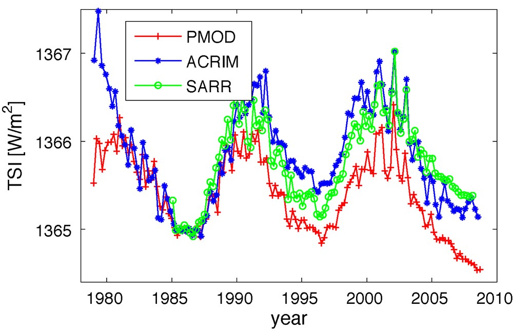
Comparison of three composites of the total solar irradiance, averaged over 81 days. The composites are: PMOD version d41-61-0807 (Fröhlich, 2006), ACRIM version 11/08 (Willson and Mordvinov, 2003), and SARR version 3/08 (Mekaoui and Dewitte, 2008). For better visibility, all curves have been shifted vertically to share the same average value for 1986–1987.
Fig. 2. Comparaison entre trois composites de l’irradiance solaire totale, moyennées sur 81 jours. Ces composites sont : PMOD, version d41-61-0807 (Fröhlich, 2006), ACRIM, version 11/08 (Willson and Mordvinov, 2003), et SARR, version 3/08 (Mekaoui and Dewitte, 2008). Par souci de lisibilité, les courbes ont été décalées verticalement et ont la même valeur moyenne entre 1986 et 1987.
Two key issues with the TSI are the origin of its variability and the reconstruction of past values. The Sun is photometrically quiet and the short-term variability mainly results from a competition between an irradiance deficit due to sunspots and an enhancement due to bright photospheric features called faculae (Fröhlich and Lean, 2004). The two effects are connected, but the variability affects different spectral bands. The secular trend in the TSI is more directly related to weak changes in brightness during spotless periods (called quiet Sun), which means that trends are best observed by comparing minima in the solar cycle. The origin of these slow brightness changes is still unclear, although it is certainly related to the solar magnetic field (Foukal et al., 2006).
A reconstruction of pre-1978 values of the TSI is of course a major issue for climate studies. There is strong observational evidence for solar surface magnetism to be the major driver of TSI changes on time scales of days to years (Krivova et al., 2003). Based on this, Fligge et al. (Fligge et al., 2000) developed a semi-empirical model for reconstructing TSI changes from the surface distribution of the solar magnetic field, using solar magnetograms inferred from solar images of the Ca K line emission. Unfortunately, few images exist before 1915, which limits the applicability of the method.
The only direct solar proxy that is sufficiently homogeneous for reconstructing the TSI back to the Maunder minimum is the sunspot number. The Maunder minimum (1645–1715) is of particular interest since the Sun was very inactive at that time and temperatures in the Northern hemisphere were unusually low (Eddy, 1976; Shindell et al., 2001). By using reconstructions of the sunspot number going back to 1610 as inputs to open magnetic flux transport simulations, several authors (Krivova et al., 2007; Lean, 2000; Wang et al., 2005) have demonstrated that the TSI was lower during the Maunder minimum than today. The uncertainty on the actual change in TSI, however, is high. Present estimates give a change in radiative forcing (the net downward radiative flux) from +0.06 to +0.3 W m−2 (Forster et al., 2007), which is equivalent to a ΔT = +0.04 to +0.18 K increase in global temperature since the Maunder minimum. The Intergovernmental Panel on Climate Change (IPCC) concludes that this bare change is insufficient to explain the observed global temperature increase (Forster et al., 2007). The same conclusions hold for reconstructions made since 1978.
For TSI reconstructions on time scales of centuries to millennia, a different approach must be used. The most reliable proxies are cosmogenic isotopes such as 14C and 10B, whose production rate is modulated by solar activity (Bard and Frank, 2006). Bard et al. (Bard et al., 2000) have shown that relative variations in the abundance of such cosmogenic isotopes are in excellent agreement with sunspot-based TSI reconstructions. There have been attempts to reconstruct solar activity up to hundreds of thousand years into the past (Usoskin, 2008). For such long periods, however, the slowly but erratically varying geomagnetic field becomes a major source of uncertainty. Discrepancies between paleomagnetic reconstructions based on different deep-sea cores are still too important to properly quantify the solar contribution 20 kiloyears and more backward (Bard and Frank, 2006).
The relatively small impact of solar radiative forcing on climate has been questioned by several. Scafetta and West, for example, used a phenomenological model to conclude that at least 50% of the global warming observed since 1900 had a solar origin (Scafetta and West, 2005; Scafetta and West, 2007). Three recurrent arguments are:
- • recent solar activity is better reflected by the TSI composite from the ACRIM group than from the PMOD group;
- • short-term statistical fluctuations and longer-term cycles have distinct effects (Scafetta and West, 2005), which may explain why such clear signatures of solar cycles (11-year, but also the weaker 90-year Gleissberg cycle) have been found in atmospheric records;
- • feedback mechanisms are not sufficiently well understood and positive feedback may be much stronger than expected (Pap et al., 2004; Stott et al., 2003).
Lockwood and Fröhlich (Lockwood and Fröhlich, 2007) argue that the PMOD composite is the most reliable, and so solar activity has not increased at the end of the 20th century. Objections against the second and third arguments have been made by climate modellers who do not see evidence for such effects in GCM, for example the comment by Lean (Lean, 2006).
Most of the TSI consists of visible and near-infrared radiation, which are primarily absorbed by oceans and land surfaces, and in the lower troposphere by water vapour and by CO2. For that reason, a direct connection between TSI change and tropospheric temperature change can be established. This direct forcing is insufficient to explain the observed temperature increase. However, several effects such as the hydrological cycle (Shindell et al., 2006) and stratospheric water vapour feedback (Stuber et al., 2001) could have an impact on the forcing-response relationship. The debate continues unabated.
3.2 The solar spectral irradiance
A significant portion of the solar radiative output does not account for a direct radiative forcing because it is absorbed in the middle and upper atmosphere where it affects photochemistry. Spectrally resolved observations are required to study these effects.
The principal features of the solar spectrum and its variability are illustrated in Fig. 3. The main result is the large relative variability in the UV band and below, which exceeds that of the TSI by orders of magnitude. In absolute terms, this spectral variability peaks in the UV between 200 and 400 nm. Below 310 nm, this radiation is strongly absorbed in the mesosphere (from 50 km to about 80–90 km), and in the stratosphere by the ozone Hartley band (Godin-Beekman, 2009). During periods of intense solar activity, the ozone concentration thus increases, heating the stratosphere and higher layers, which affects the downward radiative flux. This also impacts the meridional temperature gradient, altering planetary and gravity waves, and finally affecting global circulation (Haigh, 1994). Haigh first introduced this general picture, which is now widely accepted (Haigh, 2007; Larkin et al., 2000; Shindell et al., 2001). The main effects are a warming of the upper and lower stratosphere at low and middle latitudes, and a strengthening of the winter stratospheric polar night jet. Direct heating by absorption of the UV can explain most of the temperature response in the upper stratosphere but not in the troposphere and lower stratosphere. The final temperature response depends critically on the ozone concentration profiles and on details of the coupling mechanisms. These mechanisms are non-linear, and so a meaningful radiation budget cannot be established without resorting to GCM. These models show important discrepancies and yet, recent comparisons seem to converge toward a mean model response of up to about 2.5% in ozone and 0.8 K in temperature during a typical solar cycle (Austin et al., 2008).
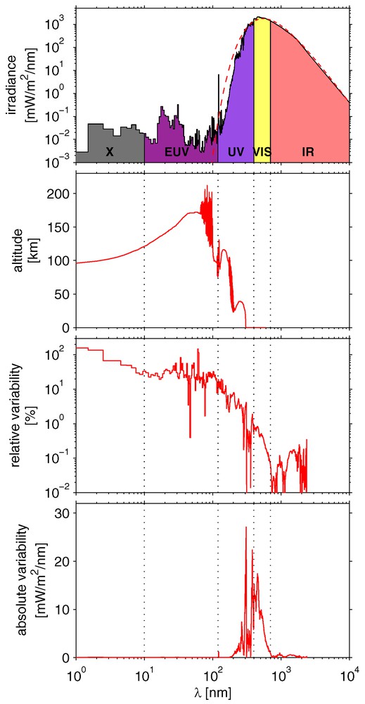
From top to bottom: the solar irradiance spectrum with (dashed) a black-body model at 5770 K, the altitude at which the UV and EUV components are predominantly absorbed (unit optical depth), the relative and absolute variability of the irradiance from solar maximum to solar minimum. All these results refer to the (Oct. 2003–Jan. 2009) time span. This plot is based on observations from SORCE/XPS, TIMED/EGS, SORCE/SOLSTICE and SORCE/SIM.
Fig. 3. De haut en bas : le spectre solaire avec en tiretés l’irradiance d’un corps noir émettant à 5770 K, l’altitude à laquelle le rayonnement UV et EUV est préférentiellement absorbé (profondeur optique unité), et les variabilités relative et absolue du spectre solaire, entre le maximum et le minimum solaire. Ces données concernent la période d’octobre 2003 à janvier 2009 et proviennent des instruments SORCE/XPS, TIMED/EGS, SORCE/SOLSTICE and SORCE/SIM.
Less than 0.01% of the total irradiance comes from wavelengths below 200 nm. This small contribution is mostly absorbed in the lowermost ionosphere, where photodissociation affects the local composition and generates heat. Because this part of the solar spectrum is highly variable, it has a noticeable effect. On time scales of hours to days, solar flares, for example, can increase the electron density by orders of magnitude (Lilensten et al., 2008). Long-term signatures of solar activity are also evident in many ionospheric parameters; the most conspicuous one is the 11-year solar cycle (Jarvis, 2006; Laštovička, 2009). The solar-cycle dependence of the height of constant plasma density in the lower ionosphere is attributed to the competing effects of a higher ionisation rate (resulting in higher plasma density at a given fixed height) and increased atmospheric heating and upwelling (resulting in lower plasma density at the same height) at solar maximum as compared to solar minimum. A slow global cooling has also been observed (Bencze, 2007), similar to that found in the meso- and stratosphere. This global cooling is most likely related to a contraction of the atmosphere due to an increasing concentration in greenhouse gases.
We conclude at this stage that the photochemical and dynamical impacts of the solar UV component have a significant leverage on the stratosphere and on climate. According to the IPCC (Forster et al., 2007), this mechanism cannot explain the temperature increase observed during the 20th century; it would require an amplification that is not reproduced by present GCM. Three important issues are:
- • to better understand the physical coupling mechanisms within the middle atmosphere and with the lower atmosphere;
- • to include in GCM originally designed for the lower atmosphere a proper description of the upper atmosphere and, reciprocally, to include in models originally designed for the upper atmosphere a better description of the lower atmosphere;
- • to improve the solar inputs to these models in order to obtain a better response of ozone concentration versus time and position.
Concerning the last issue, we note that solar spectral irradiance observations are highly fragmented and inaccurate. Indeed, such measurements must be carried out from space, where detectors suffer from degradation. An “overlap strategy” is frequently used, where successive satellite experiments are directly compared to improve their long-term accuracy. For the TSI, uncertainties of one part in 105 per annum can be obtained, whereas for the EUV–UV range, errors of more than 50% unfortunately are not exceptional.
The first continuous observations of the EUV–UV spectrum started in 2002 with the TIMED mission (Woods et al., 2005), later complemented by SORCE. Because of this severe lack of radiometrically accurate observations, most users of UV data, including climate modellers, have resigned to using proxies. The radio flux at 10.7 cm (or f10.7 index, Fig. 1) is often used in atmospheric studies, for it can be conveniently measured from ground. The MgII index (Thuillier and Bruinsma, 2001) has been advocated as a better proxy for the UV, but none of these quantities can properly reproduce the spectral variability (Dudok de Wit, 2009).
4 Orbital changes and solar diameter variations
Orbital changes and variations in the solar diameter have very little in common. Both, however, lead to a slow modulation of the solar irradiance that can be described in geometrical terms. In this sense, they fall under the preceding section. Orbital changes are well understood (Crucifix et al., 2006) and are discussed in an article by D. Paillard (Paillard, 2009).
The evidence for a variability of the apparent solar diameter has on the contrary remained elusive. Ground and space observations yield relative amplitudes of less than 0.06% over one cycle but do not agree (Thuillier et al., 2005). The effect on climate is likely to be small, but cannot be ruled out. The upcoming Picard mission, which will be launched in 2010, precisely aims at measuring the solar diameter during the rising phase of the solar cycle with unprecedented accuracy.
5 Solar impact on atmospheric electricity
Atmospheric electricity is an old field of research but its role in the Sun–Earth coupling has recently attracted considerable interest and controversy. The effect of ions on the atmosphere is discussed in more detail by E. Blanc (Blanc, 2009); here, we concentrate on the role of the Sun only.
5.1 Effect of the atmospheric current
A minute current of ∼ 2 pA/m2 permanently flows down from the ionosphere through the troposphere to the terrestrial surface, generating charges that are capable of affecting the nucleation of water droplets to form clouds. This current responds to internal but also to solar forcings, providing a mechanism by which solar activity affects various atmospheric parameters such as cloud cover, temperature and precipitation (Rycroft et al., 2000; Tinsley et al., 2007). Tinsley (Tinsley, 2008) has shown that there are at least four indirect solar inputs which modulate the process:
- • variations in the galactic cosmic ray flux, mediated by solar activity (Section 5.2);
- • solar energetic particle fluxes that are occasionally generated by intense solar flares or CME associated shocks;
- • relativistic electrons coming from the Earth's radiation belts;
- • polar cap ionospheric electric potential changes (Section 6).
The latter two are mainly induced by geomagnetic activity driven by interplanetary perturbations.
Most of the mechanisms listed above occur erratically and on time scales of days and so their long-term impact is difficult to assess. Recent advances have been made in the study of transient luminous events (Blanc, 2009), which provide an unexpected energy link between the lower ionosphere and the upper troposphere.
5.2 Effect of galactic cosmic rays
During the active part of the 11-year solar cycle the solar magnetic field and its heliospheric extension, the IMF, are generally stronger and more turbulent than around solar minimum. A stronger IMF will more successfully guide and deflect interstellar protons than a weaker IMF, with the result that the solar cycle imposes an 11-year modulation on the flux of GCR reaching the Earth's atmosphere. The contribution of cosmic rays to ion production in the atmosphere on short and long time scales is well established (Bazilevskaya et al., 2008). At present, at least three models in use describe this process: one developed in Oulu (Usoskin and Kovaltsov, 2006), another in Bern (Desorgher et al., 2005) and a third one in Sofia (Velinov et al., 2001; Velinov and Mishev, 2001). A comparison of model simulations with balloon-borne ion density measurements has shown that models and measurements are in good agreement (Usoskin et al., 2009).
Svensmark and coworkers (Svensmark, 2007; Svensmark and Friis-Christensen, 1997) promoted a mechanism in which an increased intensity of the GCR flux is, at least in part, responsible for an enhanced density of free ions and electrons in the troposphere. The free electrons, liberated by cosmic rays, assist in producing ionised aerosols which in turn should act as water vapour condensation nuclei in the troposphere. Tinsley and coworkers (Tinsley et al., 2007) suggested that a GCR flux modulation changes the aerosol ionisation which in turn changes the ice nucleation efficiency of the aerosol. In both cases, the net effect is an enhancement of the global low-altitude cloud coverage, a modification of the Earth albedo and eventually a modulation of the global tropospheric temperature in correlation with the 11-year solar activity cycle. In short, it is suggested (Svensmark, 2007) that the cloud coverage is modulated by the solar cycle, at least at heights below some 3 km.
This view is cautioned by others. Sun and Bradley (Sun and Bradley, 2002) cast doubt on the usefulness of the selection of data used by Svensmark and Friis-Christensen (Svensmark and Friis-Christensen, 1997) and demonstrate that results become different if different analysis intervals are considered. They conclude that no solid observational evidence exists for the suggested GCR–cloud coverage relation. Harrison and Carslaw (Harrison and Carslaw, 2003) and Usoskin (Usoskin, 2008) conclude that neither the GCR–cloud coverage link proposed by Tinsley and coworkers nor the one proposed by Svensmark and coworkers can be excluded but find that some elements in the chains of both mechanisms remain contentious, and they doubt whether the processes are efficient enough to contribute significantly to a modulation of low cloud formation. Sloan and Wolfendale (Sloan and Wolfendale, 2008) estimate that on a solar cycle scale, less than 23% of the 11-year cycle change in the globally averaged cloud cover is due to the change in the rate of ionisation from the solar modulation of cosmic rays.
The controversy is still going on, and the lack of accurate long-term observations of cosmic ray intensity and especially global cloud coverage presently does not allow to accept or discard a potential influence of the GCR-cloud connection on long-term changes of the tropospheric mean temperature. The CLOUD experiment that is planned at CERN should help better quantify the cloud formation rate (Svensmark, 2007). Experimental evidence gathered so far appears to suggest that on short time scales (a few days) and on interannual time scales a link between cosmic ray flux and low cloud coverage exists. The correlation between low cloud area coverage and cosmic ray induced ionisation has been found to be dependent on latitude and geographic region. It is significantly positive at mid-latitudes but poor (and possibly negative) in the tropics (Pallé et al., 2004; Usoskin et al., 2004). Depending on the time interval considered, better correlations exist over the Atlantic (1983–2000) or over the Pacific (1983–1993) (Pallé et al., 2004). Europe and the North and South Atlantic exhibit the best correlation over the period 1984–2004 (Usoskin and Kovaltsov, 2008). The pronounced regional variation of the correlation eventually results in a poor global correlation (Usoskin et al., 2004).
Let us stress again that all solar variability is eventually driven by the solar magnetic field, and so it is difficult to quantify the real contribution of each mechanism. As an illustration, Lockwood et al. (Lockwood et al., 1999) found the open solar magnetic flux to increase during the 20th century. This results in an increased shielding against GCR and possibly a reduced cloud coverage. The same open magnetic flux, however, is also strongly correlated with the TSI (Lockwood, 2001) and with the level of geomagnetic activity, both of which lead to a temperature change.
6 Atmospheric convection under quiet solar conditions
Under quiet solar conditions, the transfer of energy from the Sun into the Earth's atmosphere leads to the development of an electric current system (the solar quiet or Sq system) which consists of two components, one driven by solar electromagnetic radiation (Sq0) and the other by the interaction between the solar wind and the geomagnetic field. Note that the influence of the geomagnetic field on the motion of charged particles is rather strong such that the electrons (which above some 70–80 km altitude are little affected by collisions and are the most important carriers of ionospheric electric currents) move preferentially perpendicular to both the electric and magnetic fields (known as Hall effect).
Solar UV/EUV heating increases the scale height of the neutral constituents and causes their daytime upwelling, which is accompanied by a systematic neutral gas redistribution via tidal winds. The ionised part of the upper atmosphere between about 90 and 140 km altitude, dynamically strongly coupled to the neutral gas via collisions between ions and neutral atoms and molecules, expands and contracts with the neutral gas. As this motion takes place in the presence of the geomagnetic field, the charged particles experience a dynamo force and move along closed streamlines. They form the Sq0 current system, which is significant between northern and southern auroral latitudes but practically negligible at polar cap latitudes. The corotation electric field (due to the frictional coupling of the neutral atmosphere to the Earth rotation) exercises a strong influence at low, middle and subauroral latitudes and imposes a systematic eastward shift on the Sq0 pattern.
Seen from an observer at a fixed point in a Sun–Earth coordinate system, i.e., not rotating with the Earth (for instance, at rest in a geocentric solar magnetospheric [GSM] system), the solar wind together with the IMF create a electric field, usually termed “solar wind merging electric field” along the high-latitude magnetospheric boundary (with and denoting the solar wind bulk speed and IMF vectors, respectively). The electric field maps down to the Earth's atmosphere along geomagnetic field lines (which can be considered equipotential lines in the magnetosphere) and is observed as an electric field from dawn to dusk across the polar cap. This electric field, combined with the geomagnetic field (downward in the northern and upward in the southern polar cap) supports a Hall current from the nightside to the dayside across the polar cap, closed by return currents (known as auroral electrojets) at slightly lower but still auroral latitudes. Such return currents must flow in the ionosphere because the ionospheric Hall currents are divergence free. This is the second contribution to the Sq currents. The coupling of the atmosphere to the rotating Earth and the magnitude of the east–west component of the IMF modify the preferential orientation of the convection pattern in the sense that it may become more or less shifted, mostly in westward but sometimes in eastward direction.
Although the rate of solar radiation on the topside atmosphere depends solely on geographic latitude and longitude, the Sq current system also depends on geomagnetic latitude and longitude, as a result of the ionospheric plasma density distribution. The latter is not only governed by charge production via UV and EUV radiation but also by the electric conductivity tensor, which depends on the orientation of the geomagnetic field vector. For instance, close to the geomagnetic equator, the magnetic field is nearly horizontal. The only way to move electric charges across the geomagnetic field is along the equator as any vertical electric current would immediately be quenched by space charges accumulating at the lower and upper boundaries of the ionosphere. This effect facilitates considerably the establishment of a narrow electric current strip in the dayside upper atmosphere along the geomagnetic equator (known as equatorial electrojet).
The Sq current system is strongly dependent on season, with a remarkable increase in the summer and a decrease in the winter hemisphere. The Sq system further depends on the solar cycle; the somewhat higher average solar wind speed and the enhanced atmospheric ionisation due to more intense UV/EUV radiation and energetic particle precipitation increase the electrical conductivity and contribute to more intense ionospheric electric currents during the maximum and early declining phases of the solar cycle.
Fig. 4 (Matsushita, 1975) shows the Sq current system generated by solar electromagnetic radiation alone (Sq0, right hand side) and the combined electromagnetic and solar wind generated Sq system (left hand side).

Ionospheric Sq current system as inferred from ground-based magnetometer observations at 40 sites over the period May–June 1965. Right hand side: tidal currents only, left-hand side: combined tidal and polar cap currents. Current intensity between adjacent lines is 10 kA counterclockwise (solid) and clockwise (dotted) (Matsushita, 1975).
Fig. 4. Le système de courant ionosphérique Sq, déterminé à partir des mesures faites au sol avec un réseau de 40 magnétomètres, pour la période allant de mai à juin 1965. À droite, figurent uniquement les courants de marée, et à gauche la combinaison des courants de marée et de ceux de la calotte polaire. L’écart entre les courbes de niveau est de 10 kA. Le courant s’écoule dans le sens horaire (tiretés) et anti-horaire (trait continu) (Matsushita, 1975).
7 The impact of solar activity on the Earth's atmosphere
The steady-state conditions representing the quiet Sun are not typical for the maximum and early declining phases of the solar cycle. The impact of short-term (transient) events on the Earth's atmosphere can be profound (Kamide and Chian, 2007). Several types of eruptions are known to occur, with solar flares and CME being the most violent ones (as far as the effects on the Earth's environment are concerned). Just as under quiet solar conditions, both electromagnetic radiation and solar energetic particle fluxes play important roles for the state of the upper atmosphere under the various types of active solar conditions.
Solar flares, a bursty type of energy release, radiate broadband electromagnetic waves whose intensities are much higher than steady-state solar radiation. The rather strong X-ray component associated with flares penetrates deep into the atmosphere and enhances the ionisation level between 60 and 90 km altitude. This has deleterious effects on HF radiowave propagation.
Some solar flares and CME are accompanied by streams of very energetic protons (up to hundreds of MeV) ejected from the Sun and accelerated in the solar corona and beyond. Unlike the typical solar wind protons (≈1 keV), these high-energy protons can penetrate into the outer magnetosphere nearly unhindered by the geomagnetic field (which normally shields the Earth environment from the direct entry of solar wind particles) and propagate along the field lines toward the Earth. Protons with energies up to 10 MeV ionise the polar atmosphere at altitudes significantly below 100 km, which facilitates considerably the absorption of HF radiowaves propagating at polar latitudes (referred to as polar cap absorption [PCA]). The flare-associated proton flux may last for several days which is the time it takes to bring the plasma density back to a normal level.
A different category of solar activity, with less profound effects on the average, follows a recurrent pattern. At the boundary between low-speed (≈ 400 km/s) and high-speed (≈ 700 km/s) solar wind flow regimes, one often observes a shock front that is produced by the high-speed plasma pushing the low-speed plasma. The flow regime boundary is fixed to the solar surface, rotates with the Sun and is likely to persist for longer than one solar rotation such that the associated solar wind structures show a tendency to hit the Earth's space environment again after one solar rotation (approximately 27 days).
Fig. 5 (from NOAA-NGDC) shows, among other parameters, solar X-ray and energetic particle fluxes observed at geostationary orbit during the geomagnetic storm on 14 July 2000 which became famous as the “Bastille day storm”. On 14 July, the X-ray fluxes in both channels reach X-class intensity which is considered severe by space scientists. While the X-ray flux returns to near pre-flare intensities after several hours, the particle flux remains highly elevated for more than a day and moderately elevated for several days.

Observations by the SEM instrument onboard GOES-10 during the Bastille day storm. Top panel: soft X-ray intensity in the 0.05–0.3 nm (XL) and 0.1–0.8 nm (XS) bands. Second panel: energetic particle flux intensity. Protons > 1 MeV (I1), > 5 MeV (I2), > 10 MeV (I3), > 30 MeV (I4), > 50 MeV (I5), > 60 MeV (I6), > 100 MeV (I7); electrons > 2 MeV (E1 – mostly no data); α particles 150–250 MeV (A5), 300–500 MeV (A6). Third panel: magnetic field perpendicular to GOES orbital plane (i.e., practically in geographic northward direction). Fourth panel: neutron flux from the McMurdo neutron monitor in the Antarctic. Note the ground level enhancement at 11 UT on 14 July and the Forbush decrease (deepest in early morning of 16 July). Open and closed triangles mark the position of GOES-10 at local noon and midnight, respectively (figure generated by NOAA's National Geophysical Data Center).
Fig. 5. L’orage géomagnétique du jour de la Bastille (14 juillet 2000), observé par l’instrument SEM sur GOES-10. Le graphe du haut montre le flux de rayons X mous dans les bandes de 0,05–0,3 nm (XL) et de 0,1–0,8 nm (XS). Le second graphe montre le flux de particules de haute énergie, avec des protons > 1 MeV (I1), > 5 MeV (I2), > 10 MeV (I3), > 30 MeV (I4), > 50 MeV (I5), > 60 MeV (I6), > 100 MeV (I7) ; des électrons > 2 MeV (E1 – avec des données manquantes) ; des particules α entre 150–250 MeV (A5), 300–500 MeV (A6). Dans le troisième graphe : le champ magnétique perpendiculaire au plan orbital de GOES-10 (correspondant quasiment au Nord géographique). Dans le dernier graphe : flux de neutrons du moniteur à neutrons de McMurdo, en Antarctique. Notez l’augmentation du flux (ground level enhancement) le 14 juillet à 11 heures TU, suivie d’une décroissance de Forbush qui atteint son minimum tôt le matin du 16 juillet. Les triangles vides et pleins indiquent respectivement le midi local et le minuit local à l’emplacement de GOES-10 (figure générée par le National Geophysical Data Center de la NOAA).
Solar energetic particles can penetrate the Earth's atmosphere down to stratospheric and even tropospheric heights. For instance, chemically-induced changes in the abundance of nitric oxide constituents in the stratosphere resulting from such fluxes were observed with the UARS satellite (Jackman et al., 2006). In another case, extremely energetic solar cosmic rays associated with the intense solar X-ray flare and CME of 20 January 2005 led to a substantial ground level enhancement and an increase of the aerosol density over Antarctica as inferred from the TOMS Aerosol Index (Mironova et al., 2008).
Auroral activity, triggered by the impact of solar activity on the Earth's magnetosphere, is one of the various sources of atmospheric gravity waves. Gravity waves play a significant role in the momentum and energy budget of the mesosphere and lower thermosphere (Fritts and Alexander, 2003).
Both electromagnetic radiation and charged particle precipitation into the atmosphere can lead to a modification of the neutral air density in the upper atmosphere. Excessive UV and EUV radiation associated with solar activity, and to a smaller extent keV particle precipitation and Joule heating (caused by the motion of the ionospheric plasma forced by strong electric fields) can heat the atmosphere at the altitudes of Low Earth Orbiting (LEO) satellites – between about 300 km and more than 1000 km above the ground – thereby increasing the neutral air density at a given height and eventually leading to increased satellite drag. At the lowest satellite altitudes (300–400 km), the air density can reach several times the value typical for quiet conditions.
A connection between solar activity and the atmosphere that is specific to the Antarctic continent was proposed by Troshichev (Troshichev, 2008). The solar wind merging electric field maps, via field-aligned currents, down to the atmosphere to establish a transpolar cap electric potential whose changes can, via electric connection to the troposphere, influence the large-scale vertical circulation system that forms above the Antarctic continent in the winter season. In this circulation system, air masses descend above the central Antarctic ridge and ascend near the coast. If the vertical winds become very strong (for instance, as a result of field line merging at the magnetopause), they disturb the thermal equilibrium which results in an increased cloud coverage over Antarctica and they disturb the large-scale horizontal wind system, thereby quenching the circumpolar wind vortex. Indirect evidence for this effect was inferred from regular meteorological observations made at Antarctic stations.
8 Coupling of atmospheric layers
The coupling between the ionised and neutral gas components of the upper atmosphere up to about 140 km is a two-way process. If the electric field and the neutral wind measured in an Earth-fixed reference frame are denoted by and , respectively, the electric current density in the presence of the geomagnetic field, , is expressed as with denoting the electric conductivity tensor. An electric field (of external origin, for instance) influences the ion velocity and, via collisional coupling, the neutral gas while the neutral wind (due to pressure, gravity and the Coriolis force, for instance) is equivalent to a electric field (in an Earth-fixed frame) and influences in return the ion and electron velocities. In other words, solar energy may be transferred from the electrically charged to the neutral component of the upper atmosphere via frictional heating while kinetic energy may be transferred from the neutral to the charged component via a neutral wind associated electric field.
In addition to dynamic coupling between the neutral and electrically charged components of the ionosphere, it has become evident that different atmospheric height regions are also coupled. Planetary waves are prime candidates for linking different altitudes (Salby, 1984). They are large-scale oscillations of the lower, middle and upper atmosphere with periods preferentially (but not exclusively) near 5, 10 and 16 days. In some cases, planetary waves are generated in the lower atmosphere (troposphere and stratosphere) and propagate upward into the middle and upper atmosphere. In other cases, they appear to have been generated in the middle atmosphere and propagate latitudinally.
Goncharenko and Zhang (Goncharenko and Zhang, 2008) conclude that seasonal trend, solar flux and geomagnetic activity cannot account for temperature variations in the thermosphere which they had observed during an incoherent scatter radar campaign in January–February 2008. They suggest that the variations are associated with stratospheric warming and hence demonstrate a link between the lower and the upper atmosphere. Yiğit et al. (Yiğit et al., 2008) demonstrate the penetration of gravity waves and subsequent momentum deposition from the lower troposphere and stratosphere to the middle thermosphere.
Supported by the observational evidence acquired over the years, it became clear that kinetic and electromagnetic coupling between atmospheric layers exists and the need for developing coupled atmosphere–thermosphere–ionosphere–plasmasphere models emerged. As a consequence, GCM of the terrestrial upper atmosphere have evolved. About a decade ago, the time-dependent three-dimensional Coupled Thermosphere Ionosphere Plasmasphere (CTIP) model was developed (Millward et al., 1996). The CTIP model consists of three distinct components, a global thermosphere model, a high-latitude ionosphere model and a mid- and low-latitude ionosphere/plasmasphere model.
The Coupled Middle Atmosphere and Thermosphere model (CMAT) is one of the advanced models ultimately derived from the CTIP model. Its range of validity was originally extended down to 30 km altitude (Harris, 2001) and a further improved version (CMAT2 (Cnossen et al., in press)) extends from exospheric heights (from 104 km altitude for the ionospheric flux tubes) down to 15 km altitude. The extensions to CTIP mean that lower atmosphere dynamic effects such as gravity waves can be included, and conversely the effects of ionospheric inputs such as auroral precipitation on middle and lower atmosphere can be examined.
A Thermosphere General Circulation Model (TGCM) family, developed at the National Center for Atmospheric Research by Richmond et al. (Richmond, 1992), comprises three-dimensional, time-dependent modules representing the Earth's neutral upper atmosphere. Recent models in the series include a self-consistent aeronomic scheme for the coupled Thermosphere/Ionosphere system, the Thermosphere Ionosphere Electrodynamic General Circulation Model (TIEGCM) and the TIME-GCM, which extends the lower boundary to 30 km and includes the effects of the prevailing physical and chemical processes.
Optical phenomena such as lightning-induced sprites, jets and elves and the electromagnetic fields associated with them have become a topic of intense study over the last decade. They are of too small a scale to be handled properly by global circulation and coupling models. This kind of electromagnetic activity is discussed in a companion article by E. Blanc.
9 Conclusions
Solar radiation is by far the most intense source of energy supplied to the terrestrial atmosphere, and there is a wealth of evidence in favour of the response of atmospheric parameters to solar variations. Most of the attention has focused so far on the sole variability of the TSI, which gives a simplistic view of the complexity of the solar driver. Indeed, solar variability manifests itself in a variety of different (but coupled) mechanisms; most of the underlying feedback mechanisms remain poorly known, which hampers the quantification of individual processes. For that reason, there has been and is still much debate about the real impact of solar variability on climate. According to the IPCC (Forster et al., 2007), over the last century, this impact has most likely been small as compared to anthropogenic effects.
There are several important working fronts as far as the Sun–Earth connection is concerned. Most GCM whose development started in the lower atmosphere still largely ignore the upper part of the atmosphere on which solar variability has the largest impact. One obvious issue is therefore the upward extension of these models, and a better description of the mechanisms by which the upper layers may couple to the stratosphere and eventually to the troposphere. This also involves a better understanding on how solar variability affects regional climate data. On the other hand, GCM models, like the CITP which started from the thermosphere, face the challenge of an appropriate downward extension to the stratosphere (and eventually the troposphere).
A second issue is the definition of reference spectral irradiance in the EUV and UV bands for different levels of solar activity. These bands have an important leverage of the middle atmosphere and the reconstruction of past levels is still lacking today. In all these reconstruction attempts, however, one should be careful against inbreeding of models.
A third issue is the understanding of the microphysics associated with atmospheric electricity and in particular the quantitative role of ions and electrons for stimulating the production of water vapour condensation nuclei. All three issues involve a much closer interaction between the space and atmospheric communities, which is definitely the highest priority of all.
Acknowledgements
During the preparation of this paper, JW benefited from a grant provided by Le Studium, Agence régionale de recherche et d’accueil international de chercheurs associés en région centre, France. We also gratefully acknowledge the numerous institutes and teams that provided the experimental data we used in the plots.
1 Space weather mostly deals with short-term impacts and forecasting of solar activity, with a particular focus on its societal effects: impacts on space systems, navigation, communications, ground technology, etc.
2 Defined here as (maximum − minimum)/time average.