

1 Introduction
The geologists in the 18th to 19th centuries were fully aware that the Earth has undergone many dramatic changes through its history. This was, in particular, attested by the succession of the different animal or vegetal fossil species in the geological record. But it is through the discovery of glacial ages, in the middle of the 19th century that the idea of a changing climate became a true scientific subject. Indeed, glaciers have carved the landscape of many regions in Europe and in northern America and have left their undisputable traces such as moraines, or erratic blocks, in areas that are nowadays devoid of any ice. This led Louis Agassiz (Agassiz, 1838) and other geologists (Bard, 2004) to suggest that climate on Earth could have been much colder than today at some older periods of time, at least in the northern hemisphere.
The point of view of the scientists at that time on glacial ages was quite different from today. In particular, it was largely associated with a “catastrophist” perspective of the Earth history, which was punctuated by great floods and other cataclysms. For them, climate was first of all a result of the Earth geography and topography. The idea of continental drift came much later in the 20th century, and the early geologists were interpreting their observations mostly in terms of vertical motions: mountain rising, erosion, changing sea level… Under the influence of Charles Lyell (Lyell, 1830), all these changes became slow and progressive. Catastrophism was replaced by gradualism, which postulates that changes of the Earth surface in the past are the same as those occurring today, like erosion, but applied on extremely long durations. This new point of view was strongly opposing any external influence (in particular divine one) on the evolution of the Earth. This probably largely explains the strong opposition of geologists to the very first astronomical theories of glacial ages.
“But though I am inclined to profit by Croll's maximum eccentricity for the glacial period, I consider it quite subordinate to geographical causes or the relative position of land and sea and abnormal excess of land in polar regions”
(C. Lyell to C. Darwin, 1866)
The idea that climate results primarily from Earth geography and topography is of course well founded, as emphasized by the etymology of the word climate (from the Greek κλιμα = tilt, or height of the sun above the horizon, which corresponds to the idea of geographic latitude). Still, the physical principles determining climate were also mostly established during the 19th century, with, for instance, Joseph Fourier (Fourier, 1822) who established the laws of heat diffusion, and who explained how heat was redistributed at the Earth surface by two fluids, the atmosphere and the ocean. He also discussed of the critical role of the greenhouse effect. It is in this historical context that the two main theories of glacial ages were forged: the astronomical theory and the changing concentration of atmospheric carbon dioxide.
2 Astronomical theories versus atmospheric carbon dioxide ones
The first astronomical theory of glacial ages was formulated by Joseph Adhémar (Adhémar, 1842). Indeed, as will be discussed in the following, the precession of equinoxes was well known by astronomers since the Antiquity. It was referred to as the “third motion of the Earth” by Nicolas Copernic, the two first ones being the daily rotation and the yearly revolution around the Sun. Since diurnal and seasonal temperature changes are obvious facts, it made a lot of sense to look for climatic consequences of this “third motion”. A consequence of the precession of equinoxes is to change the location of the perihelion (the point on the Earth orbit nearest to the Sun) with respect to seasons. Today, the Earth is nearest to the Sun on the 3rd or 4th of January. This date changes slowly around the year in a 21,000 year cycle. About 10,500 years ago, the Earth was therefore closest to the Sun in July, and far from it in January. Adhémar put forward that these changes should modify climate. More precisely, today's northern hemisphere winters are close to the Sun, whereas southern hemisphere ones are far from it. Adhémar suggested that this situation explains why there is no large ice sheet in the north, because of mild and short winters, while there is a large one, Antarctica, in the southern hemisphere. The situation was, according to him, exactly reversed 10,500 years ago, which should explain the occurrence of ice ages in the north, as evidenced by geological data. Adhémar's theory was criticised for many reasons, some largely unfounded. However, it is first of all on a simple astronomical logical argument that it was dismissed by his opponents Charles Lyell and Alexander von Humbolt. Indeed, this precessional mechanism is rigourously antisymmetric with respect to hemispheres, but also with respect to seasons. It can be easily demonstrated that, for instance, if winters receive less energy, this is exactly compensated by excess energy received in summer. If the seasonal contrast may change with precession, the total annual energy received from the Sun does not change.
James Croll (Croll, 1867) puts forward a solution to this problem since, if the astronomical forcing is indeed antisymmetrical with respect to seasons, climatic processes are likely not so. In particular, snow accumulation occurs mostly in winter, while the melting of ice occurs mostly in summer, and there is no guarantee that an excess snow due to a colder winter should be exactly compensated by an excess melting in a warmer summer. Croll insisted strongly on the role of snow accumulation during winters, in such a way that the theory of Adhémar remained essentially valid: stronger or longer winters were supposed to lead to increased ice volume and glaciation. Furthermore, the recent developments of celestial mechanics (in particular by Pierre Simon de Laplace and Urbain le Verrier) led Croll to introduce explicitly the effect of the changing eccentricity of the Earth orbit. Eccentricity strongly modulates the effect of precession. Indeed, for a circular orbit, there is simply no perihelion or aphelion, and the larger the eccentricity, the stronger the differences between a “mild winter” at perihelion, and a “cold winter” at aphelion. According to Croll, large glaciations were therefore associated with maximum eccentricity, which led him to suggest an age of at least 80,000 years for the last glaciation, with an even greater glacial event about 240,000 years ago (Croll, 1867). Though the theory of Croll was much more solid and complete, he did not succeed to convince his contemporaries. Still, the alternating glacial–interglacial sequences found in some sedimentary records were clearly in favour of a more or less cyclic phenomenon. However the first available dating elements, by extrapolating erosion rates or counting lake-sediment varves, were clearly indicating a much more recent glaciation.
It was half a century later that Milutin Milankovitch (Milankovitch, 1941) formulated the astronomical theory than is considered valid still today. The main problem of Croll's theory is to consider winter as the critical season for the evolution of ice-sheet. From observations made on mountain glaciers, Milankovitch demonstrated that summer melting is much more critical for the ice mass balance than winter snow accumulation, and his theory is therefore based on summer insolation. This is exactly the opposite of Adhémar's or Croll's suggestions. Furthermore, Milankovitch also computed explicitly a third astronomical parameter relevant for the insolation at the top of the atmosphere: the obliquity of the Earth axis, which corresponds to its tilt with respect to the orbital plane. This sets the basis of the current astronomical theory of climate.
The role of the atmosphere acting as a greenhouse was already understood at that time, but it is John Tyndall who measured the infrared absorption and emission of the different gases present in the atmosphere. He showed that nitrogen and oxygen, the main constituents of the atmosphere, were mostly transparent in this part of the spectrum, and that the greenhouse effect was caused entirely by trace gases like water vapor, carbon dioxide, methane or ozone. Jacques Joseph Ebelmen (1845), a French geologist, was probably the first to put forward that changes in the atmospheric carbon dioxide concentration were possibly the cause of past climatic changes (Bard, 2004). The measurements performed by Tyndall (1861) (Tyndall, 1861) allowed to quantify this mechanism, and Tyndall thus suggested that the climatic changes found by geologists could be easily explained by changes in greenhouse gases concentrations. These ideas were also adopted by the American geologist Chamberlin, who described the succession of at least five glacial periods in the United States. But it is the chemist Svante Arrhenius who further developed this theory by computing explicitly the climatic effect of atmospheric CO2 changes. From available geological data on the location of moraines during glacial times, he evaluated the cooling to be about 4 or 5 °C, and he computed that such a cooling could be caused by a reduction of atmospheric CO2 by about 40%. These estimations are astonishingly close to the measurements obtained from air bubbles in Antarctic ice cores, which demonstrate that CO2 was indeed about 30% lower during glacials compared to interglacials. Besides, current estimates of the glacial temperatures agree fairly well with Arrhenius numbers.
It is quite interesting to note that, since the middle of the 19th century, these two theories of glacial ages have been alternatingly put forward, with palaeoclimatic data favouring successively one hypothesis then the other. If the astronomical theory became the standard one in the 1970s through the discovery of astronomical periodicities in the climate record, the greenhouse gases data from Antarctic cores demonstrates that the alternative point of view is also quite valid. Today, the synthesis of these two competing theories remains to be built. But before drawing a sketch of such a new synthesis, it is worth detailing how orbital parameters are influencing Earth climate in several different ways.
3 Astronomical parameters and insolation forcing
3.1 Eccentricity
According to Kepler's first law, the Earth's orbit is an ellipse. It is characterized by a size parameter, the semi-major axis, traditionally represented by a, and by a shape parameter, the eccentricity e. Three other parameters are defining its absolute orientation in space, two of which are defining the orbital plane (the inclination i with respect to a reference plane, and the longitude of the ascending node Ω, defined by the intersection between these two planes), and the third one representing the location of the perihelion, the longitude π. As soon as a system is composed of more than two bodies (the Sun and the Earth) like the solar system, then the motion is no more a fixed ellipse, and there is actually no analytical solution to the N-body celestial mechanical problem, when N is larger than 2 (Fig. 1). The computation of planetary motions on long time scales is therefore a perturbative one or a numerical approximation. The notion of orbit remains valid since perturbations are only second order. They become significant only on rather long time scales. The motion is therefore better described as a slowly changing elliptic orbit. The perturbations induced by the other planets are not affecting the size a of the ellipse, but only its shape e and its orientation (i, Ω, π). Consequently, a is assumed constant through time, at least over the last hundreds of millions of years (neglecting solar mass loss and other small effects). Besides, the orientation of Earth's orbit in space has a priori no climatic consequence over the solar radiation received on top of the atmosphere (though some people may have claimed otherwise (Müller and McDonald, 1995)). As a result, the only remaining orbital parameter able to affect solar radiation is the eccentricity e.
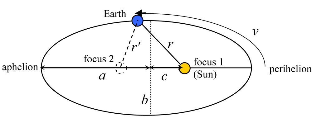
An ellipse can be mathematically defined by the location of points whose sum of distances to foci is constant: r + r’ = 2a. Eccentricity is defined by e = c/a. The semi-minor axis b is then given by Pythagora's formula: b = a(1 − e2)1/2.
Une ellipse est définie mathématiquement par le lieu des points dont la somme des distances aux foyers est constante: r + r’ = 2a. L’excentricité est définie par e = c/a. Le demi-petit axe est alors donné par la formule de Pythagore : b = a(1 − e2)1/2.
Eccentricity is defined by the ratio between the centre-to-focus extent c with respect to the semi-major axis a. Today, eccentricity reaches 0.0167, but it changed between values close to zero and values close to 0.06, with pseudoperiodicities of about 100,000 and 400,000 years.
Eccentricity does change the global annual mean energy received by the Earth. Indeed, the semi-major axis being constant, the mean Earth–Sun distance depends directly on eccentricity. Kepler's second law (which corresponds to the conservation of angular momentum) can be written as:
By integration over a complete year, this leads to the formula of the “Solar constant” S0, defined as the mean energy received by the Earth, which depends directly from the eccentricity:
This of course depends on the energy S received at a distance a from the Sun, which will be assumed here constant, though changes in solar activity are known to occur, at least on decadal time scales and probably also on centenial ones. A larger eccentricity leads to a flatter ellipse, in annual mean closer to the Sun, and therefore leads to a higher energy received by the Earth S0. Still, changes are very small since, using the above formula, the maximum eccentricity e = 0.06 leads to S0 = 1.0018 S, which represents only a 0.18% increase, a figure fully comparable with the changes associated with solar activity mentioned above. To first order, these changes have consequently only a negligible effect on climate. But, as we will see later on, eccentricity modulates the effect of precessional changes, which have a much larger magnitude. The effect of eccentricity on climate is therefore mostly indirect.
It is worth mentioning that the solar system is chaotic. This means that the computation of orbital parameters, and among them eccentricity, is possible only for periods of time not too remote in the past or in the future. Indeed, errors are increasing exponentially through time and a precise computation beyond about 20 or 30 millions of years is not possible, which is in fact quite short compared to the age of the Earth. Beyond this duration, changes in eccentricity are still similar (with identical pseudoperiodicities near 100,000 and 400,000 years) but it becomes impossible to ascertain if, for instance, 600 millions years ago eccentricity was at a minimum or at a maximum. In other words, the phase of oscillations becomes unpredictable.
3.2 Obliquity
Beyond orbital parameters, we also need to account for the orientation of the Earth's axis with respect to the orbital plane, or ecliptic. This is given by two axial parameters, the obliquity ɛ which represents the tilt of the Earth's axis compared to the ecliptic, and the precession of the equinoxes, which relates to its absolute position with respect to the stars. The Earth's axis orientation is mostly changed by the differential attraction of the Moon on Earth's equatorial bulge. Indeed, the Earth is slightly flattened due to its rotation, and the Moon's gravitational attraction is not exactly symmetrical: the equatorial bulge is tilted compared to the Moon's orbit, which induces a torque on Earth's axis and changes its orientation. In contrast to orbital parameters like eccentricity, which depends only on point mechanics, the axial parameters (obliquity and precession) also depend on the Earth's shape. This introduces additional uncertainties and potential errors. The characteristic duration beyond which predictions for axial parameters become impossible is therefore probably shorter that for eccentricity, and difficulties arise already after several millions of years. In particular, the shape of the Earth changes slightly throughout a glacial cycle with huge ice masses being accumulated at high northern latitudes. It was suggested that this could influence the computation of axial parameters after a few million years. Similarly, internal mantle convection in the Earth may also redistribute masses within the Earth in ways than cannot be accounted for in astronomical computations. As a result, the phase of obliquity and precession are uncertain in the remote past and future.
Today, obliquity is ɛ = 23°27’, which defines the latitude of polar circles (67°33’ north and south) and tropics (23°27’ north and south). This value oscillates between extremes of 21.9° and 24.5°, with a pseudoperiodicity of about 41,000 years. We easily grasp that any change in obliquity will have climatic consequences by modifying the extent of these polar and tropical geographic domains. As an illustration, in Taiwan, in the county of Chiayi (Jia-Yi), there is a monument marking the location of the tropic of Cancer since about the last century. However, the current decrease in obliquity, at a pace of about 0.46 arcsecond per year, induces a shift of the tropics by about 14.4 m each year, more than a kilometer since the building of this first monument. The Taiwanese have therefore built regularly new smaller monuments to follow the southward moving tropic of Cancer.
If the global mean radiation received by the Earth is unchanged, its geographic distribution depends on obliquity. More precisely, the annual mean solar radiation received at the top of the atmosphere in a given location depends mostly of obliquity (and slightly of eccentricity through its global effect). An increase in obliquity ɛ translates into an increase of the solar radiation received at high latitudes, and a decrease in the tropics. We can compute, on the equator and on the poles:
If the winter solstice insolation is always null at the pole, the summer solstice one varies between Wsummer (pole) = 0.373 S and Wsummer (pole) = 0.415 S, when ɛ changes from 21.9° to 24.5°. This represents a 4% increase, i.e., more than 50 W.m-2. This is certainly not negligible. Besides, in contrast to the precessional effects that we will examine below, the effect of obliquity on insolation is symmetrical with respect to the equator. In other words, in contrast to Adhémar's theory which was based on precession only, climatic changes associated with obliquity changes should be synchronous in both hemispheres.
3.3 Precession
As mentioned in the introduction, the precession of equinoxes is known since the Antiquity. This “third motion of the Earth” corresponds to a slow drift of the polar axis with respect to the fixed stars. Its discovery is generally attributed to Hipparque (130 BC) who estimated it to about 1° per century (or a periodicity of 360 centuries), which is reasonably close to its actual value of 1.397° per century (or a periodicity of 25,765 years). It seems likely than this shift was even known to the Egyptians much earlier, since they were changing the orientation of some monuments according to this drift. But it is necessary to distinguish the precession of equinoxes and the climatic precession. Indeed, the absolute orientation of the Earth's axis with respect to stars in not relevant for climate. However, when this axis is oriented in a different way, the same is true for the equatorial plane of the Earth. Equinoxes are precisely defined by the intersection of the equatorial plane and the orbital plane. The precession of equinoxes corresponds therefore to a drift of this line among the stars in the zodiac, thus its name. Today, the Sun is in the Fish constellation (Pisces) at the spring equinox, thus defining what astronomers are calling the vernal point γ. It was in the Ram (Aries) during Greek times and in the Bull (Taurus) during the Egyptian epoch. This succession has probably strong symbolic links, through astrology, with religions (the bull, the Hebrew ram, then the Christian fish). The vernal point and the location of seasons on the Earth orbit thus moves together with the precession of equinoxes. The orbit being elliptic, seasons will then occur at changing distances from the Sun, depending on their situations compared to perihelion and aphelion. The climatic effect of precession will be obtained through this relative location. But the perihelion is also moving with respect to the stars, as mentioned above (this is the π orbital parameter) according to the “precession of the perihelion”. The combination of these two motions is obtained by defining the climatic precession, noted ϖ (“cursive pi”), as the angle between the vernal point and the perihelion. If the vernal point moves around the sky in about 25,700 years, the perihelion does so in 112,000 years. These motions being in opposite directions, they combine into a mean climatic precessional cycle of 21,000 years (1/25.7 + 1/112 ∼ 1/21).
But a further complication is associated with the climatic precession ϖ (Fig. 2). Indeed, for instance, when the orbit is circular (e = 0), the perihelion does not exist anymore, and ϖ is undefined. Furthermore, the larger the eccentricity e, the stronger the climatic effects associated with changes in ϖ, since the Sun–Earth distance should change more between its maximum a(1 + e) (aphelion) and its minimum a(1 − e) (perihelion), while this effect vanishes when e = 0. It is therefore convenient to introduce the “climatic precession parameter” e sinϖ, which vanishes when ϖ is undefined (e = 0) and which increases with e. Mathematically, this corresponds simply to using the two parameters (e cosϖ , e sinϖ) instead of (e,ϖ), which is a change of coordinates, from polar to Cartesian ones. In this precessional parameter e sinϖ, the effect of precession is thus modulated by eccentricity, which can also be seen on the insolation formula given below. A periodicity doubling then occurs (actually, a multiplication of frequencies, since the eccentricity e contains itself many periodic terms). Indeed, if e varies with a single 100,000 year period like, for instance, the expression |e0 cos(t/200)|, and if ϖ consists of a simple 21,000 year cycle, we can deduce that:
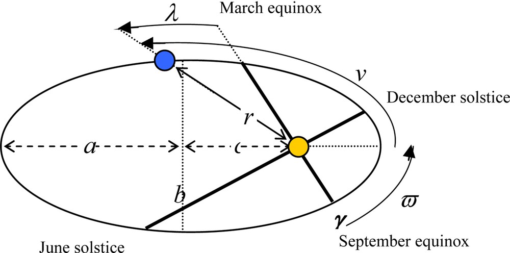
The vernal point γ is defined by the location of the Sun at the March equinox (geocentric viewpoint), which corresponds therefore on this figure to the location of the Earth at the September equinox (heliocentric viewpoint). The reference point traditionally used for λ (March equinox) is therefore the opposite of the one used for ϖ (γ). Note that it is more appropriate to refer to “March” or “September” equinoxes, which is a denomination valid in both hemisphere, in contrast to “Spring” or “Autumn” (and similarly for the solstices).
Le point vernal γ est défini par la position du Soleil à l’équinoxe de mars (point de vue géocentrique), ce qui correspond sur la figure à la position de la Terre à l’équinoxe de septembre (point de vue héliocentrique). Le point de référence utilisé habituellement pour λ est donc opposé à celui utilisé pour ϖ (γ). Notons qu’il est plus approprié de parler des équinoxes de mars et septembre, dénomination valide pour les deux hémisphères, plutôt que des équinoxes de printemps et d’automne (et de même pour les solstices).
Therefore the associated periodicities of 19,000 years and 23,000 years (since 1/21 + 1/200 ∼ 1/19 and 1/21 – 1/200 ∼ 1/23). When these periodicities were detected in oceanic paleoclimatic records, it was the strongest evidence ever in favour of the Milankovitch theory.
3.4 Computing insolation and calendar problems
Knowing the three astronomical parameters e, ɛ, ϖ, it is just a matter of simple trigonometry to compute the radiation received by the Earth at any location (latitude φ) and any season of the year. It is convenient to define the mean daily insolation: given an orbital location through its longitude λ, the angular position measurement usually with respect to the spring equinox (so than λ = 90° at the summer solstice or λ = 270° at the winter solstice), it is assumed that λ does not change throughout the day, as well as the astronomical parameters. Only a full Earth rotation is taken into account, which leads to the following result. With:
the mean daily insolation at latitude φ and orbital position (time of the year) λ is given by:
In this formula, three terms are present: first, the solar constant S (or more precisely, the solar radiation at the distance a from the Sun which is slightly different from the “solar constant” S0); second, a term corresponding to the Earth–Sun distance, which depends on the time of the year (λ), on the climatic precession (ϖ) and on eccentricity (e); finally, a third geometrical term which includes the time of the year (λ), obliquity (ɛ) and latitude (φ). In particular, the last (geometrical) term is unchanged by changing simultaneously φ in -φ and λ in λ + π (changing hemispheres and seasons). In other words, the precessional forcing is antisymetrical with respect to hemispheres. Besides, as already mentioned, we see that the integral over the year (between λ = 0 and 2π) does not depend on precession ϖ.
In this formula, it is worth noticing that longitude λ represents the location of the Earth on its annual cycle, but λ is not exactly proportional to time. Indeed, when the Earth is close to the perihelion, it moves faster and λ then changes more rapidly than when Earth is at the aphelion. More precisely, the ellipse equation in polar coordinates (centered on the Sun) is:
Kepler's 2nd law () leads to:
which can be integrated analytically into the so-called Kepler equation:
Since the duration of the seasons changes with ϖ, this raises a difficulty to define a calendar. Indeed, our calendar is not inadequate in face of the current value of ϖ with winter months having slightly less days than summer months (DJF: 90,25 d.; MAM: 92 d.; JJA: 92 d.; SON: 91 d.) somewhat in accordance to the astronomical seasons (winter: 89.0 d.; autumn: 89.8 d.; summer: 93.6 d.; spring: 92.8 d.). When using palaeoclimatic data, it is relevant to use an astronomical definition of seasons based on solstices and equinoxes, but model simulations are performed on a temporal seasonal axis. Since seasons have different durations, the imposed seasonal forcing is therefore phase-shifted at some times of the year. Usually, model-seasons are defined using a fixed number of days (either one quarter of the year, or using the current calendar), with the spring equinox taken as the reference point. There is consequently a significant phase-shift in autumn which can reach up to one or two weeks, and the monthly or seasonal climatic means are potentially strongly influenced by this bias. If the alternative is to analyze model results in terms of astronomical seasons, it is unfortunately far from being a common practice.
3.5 Which astronomical forcing for climate?
Milankovitch theory states that “summer” insolation is the critical forcing acting on the evolution of northern hemisphere ice-sheets. But should we use the daily insolation defined above at a particular summer day (like the summer solstice for instance)? Or should we integrate this quantity over the whole summer season? Or over some other interval [λ1, λ2]? Or some other temporal interval? Or should we use every day of every season, applied to an explicit physical model of the coupled climate ice-sheet system? If this last proposition is obviously the most pertinent one, it is quite difficult to apply in practice, and a simple formulation of the astronomical theory remains a very useful tool to understand its foundations.
While Milankovitch used a seasonal averaged value, the most current practice is to use the insolation at a given summer day. The standard forcing is therefore the daily insolation WD taken at 65°N at the summer solstice (λ = 90°, φ = 65°). But insolations averaged over longer periods of time may still be useful. Since the Earth's motion is not uniform, care must be taken to perform a temporal integration over some orbital interval [λ1, λ2], which leads to elliptic integrals that can now be easily evaluate numerically. Still, it has been recently suggested by Huybers (2006) (Huybers, 2006) that a much more appropriate simplified forcing is the integral of insolation above a given critical value, since a critical energy input corresponds to the limit between the melting or absence of melting of ice during summer, at a temperatures above or below the freezing point. Such an integral corresponds closely to what glaciologists traditionally use as model input, which is an integral of positive temperatures (positive degree-days or PDD). It is interesting to note that the relative weight of 23,000 and 41,000 years periodicities is quite different with such a definition of the astronomical forcing, pleading for a more prominent role of obliquity on climate than usually assumed.
4 Successes and pitfalls of the astronomical theory
During the first half of the 20th century, glaciations were mostly understood as four specific stratigraphic events in the Quaternary records (Günz-Mindel-Riss-Würm), not necessarily as a regular or periodic phenomenon. The number of glaciations increased quite dramatically with the publication of several continuous palaeoclimatic marine records in the 1950s Emiliani (Emiliani, 1955), who performed the first isotopic measurements applied to palaeoclimatology. This revived the hypothesis of a periodic external influence, but the time scale of this new set of data was poorly constrained. The Milankovitch theory became well accepted only when the astronomical periodicities were unambiguously found in palaeoclimatic records, as shown in a famous paper by Hays et al. in 1976 (Hays et al., 1976). This was made possible in the 1970s when absolute chronological information became available to geologists through the use of radio-isotopes (Broecker, 1966; Broecker et al., 1968), and when Earth magnetic reversals where identified in marine records and used as stratigraphic tools (Opdyke et al., 1966). Furthermore, decisive progresses became also available concerning the computation of astronomical parameters in the geological past through the use of computers (Berger, 1978).
If astronomical frequencies are indeed present in palaeoclimatic records, it remains to ascertain that a simple relationship links astronomy and climate, at least in a statistical way. Several techniques have been used, like the coherence which represents a correlation coefficient in the spectral domain. Results are clearly indicating a strong connection between the high latitude summer insolation forcing and the glaciation records for the obliquity periodicities (41,000 years) and the precessional ones (23,000 and 19,000 years). The link between insolation and climate in these frequency bands can be interpreted as a quasi-linear one, as shown by Imbrie et al. (1992) (Imbrie et al., 1992). Another way to illustrate this strong relationship is to examine the amplitude modulation both in the external forcing and in climate at these two frequencies. As shown of Fig. 3 for the obliquity band, the larger the forcing, the more important the climatic signal.
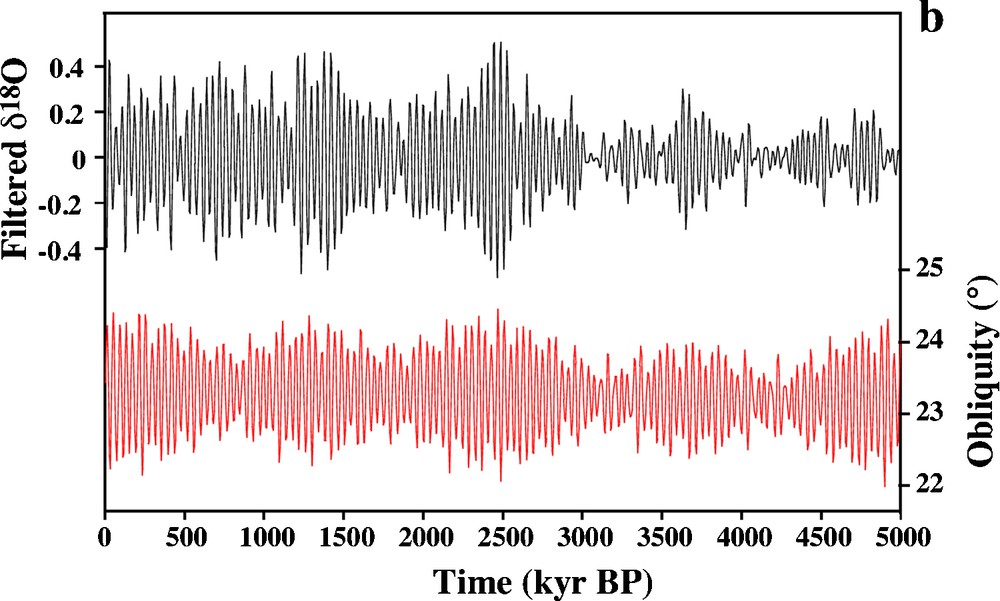
Isotopic record (ODP 659) from (Tiedemann et al., 1994) filtered at 41,000 years on the top, compared to obliquity variations from (Laskar et al., 1993) on the bottom. The amplitude modulation is very similar in both series.
Enregistrement isotopique (ODP 659) d’après (Tiedemann et al., 1994) filtré à 41 000 ans (en haut), comparé aux variations d’obliquité (Laskar et al., 1993) (en bas). La modulation de l’amplitude est similaire pour les deux séries.
This close relationship between astronomy and climate, at least at these two periodicities, can then be used for dating long-term climate records in the past. Indeed, a persistent difficulty of palaeoclimatic reconstruction concerns their chronology. If absolute dating can be obtained through radioactive isotopes (using methods like 14C, 40K/39Ar, 40Ar/39Ar, U/Th…), these measurements are scarce and difficult to obtain. Besides, they are associated with significant uncertainties, which increase at least linearly with time. For instance, if a 1% error on an age estimation corresponds to a good measurement, this still translates into a 10,000 year uncertainty when applied to a one million year old sample. It is therefore tempting to use the astronomical theory and to associate each palaeoclimatic cycle to a corresponding one in the forcing, in particular concerning precessional and obliquity cycles. When such an identification is possible, which is in fact quite common, then the associated error is much smaller, since it is restricted to the phase relationship between the astronomical forcing and the climatic response, that is a few thousands of years, even when looking millions of years into the past. The construction of such a precise chronological frame for a substantial part of the Earth history is still an ongoing work (Shackleton et al., 1999). But it is then the chaotic nature of celestial mechanics, as mentioned earlier, that starts to become a major difficulty, and astronomers may therefore use geological information to better constrain their knowledge of the parameters of the solar system (Pälike et al., 2004).
But what is true for 41,000 and 23,000 years cycles is no more valid for the major glacial–interglacial cycles that occur every 100,000 years. These major cycles are strongly asymmetric with a rather slow glaciation phase during which the ice-sheet tends to grow up to its maximum, and a much faster deglaciation lasting about 10,000 years only, that palaeoclimatologists are calling “terminations”. Even in the 1970s, it was quite clear that this saw-tooth structure would not fit easily in the astronomical framework (Broecker and van Donk, 1970). This difficulty is described on Fig. 4.
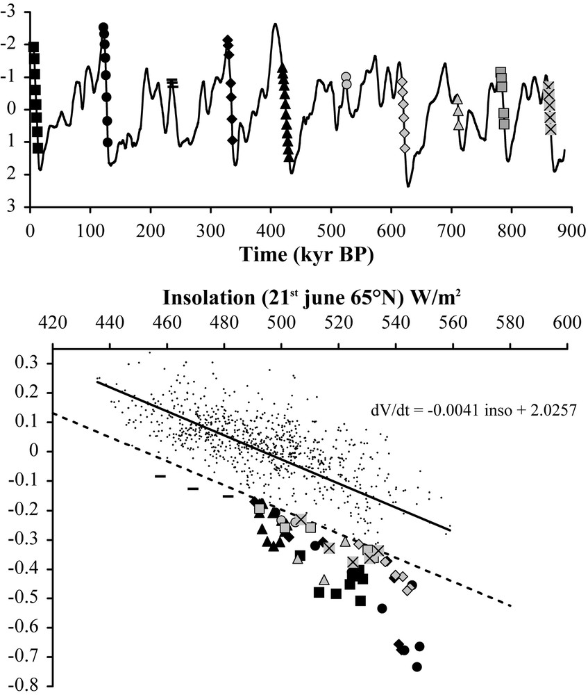
Top: the normalized SPECMAP record (Imbrie et al., 1984) used as a proxy for the global ice volume. Bottom: the derivative of this ice volume (using the difference between consecutive points) plotted against the standard Milankovitch forcing. The success of the Milankovith theory corresponds to the good correlation observed for most points on this graph. Interestingly, some points shown with symbols lie significantly below the regression line. These points are precisely those corresponding to the terminations that occur about every 100,000 years, as shown on the top curve.
En haut : enregistrement SPECMAP normalisé (Imbrie et al., 1984) comme proxy du volume des calottes de glace. En bas : la dérivée de ce volume de glace (différence des points consécutifs) en fonction du forçage de Milankovitch habituel. Le succès de la théorie de Milankovitch correspond à la bonne corrélation obtenue pour la plupart des points de ce graphique. De façon intéressante, certains points (avec des symboles) sont significativement en dessous de la droite de régression. Ces points correspondent aux terminaisons qui surviennent tous les 100 000 ans, comme montré sur la courbe du haut.
Besides, there is no statistical link (coherence or amplitude modulation) between these main climatic cycles and the eccentricity forcing. The very notion of well-defined 100,000 cycles is even problematic, since these large changes are existing only for the last million years. There is thus only about 10 such large glacial-interglacial, which makes it difficult for statistical methods to specify a well-defined periodicity. Furthermore, it appears that the duration between successive terminations is not so regular as shown in Table 1, and it has been suggested that it was more significantly associated with a multiple of the obliquity period (2 × 41 = 82 ka, or 3 × 41 = 123 ka) (Huybers and Wunsch, 2005). Besides, as mentioned earlier, eccentricity changes have only a marginal effect on the energy received by the Earth. It is therefore necessary to suggest more complex processes to obtain a climatic response in this frequency band. The simplest mechanisms involve thresholds in the climatic system, with a different mode of operation during glaciations and deglaciations. Such a strategy can be outlined using conceptual models.
Durée des 6 derniers cycles délimités par les terminaisons successives (Raymo, 1997). La cyclicité moyenne est proche de 100 000 ans, mais les durées peuvent être significativement différentes d’un cycle à l’autre, en moyennant sur différents enregistrements, ce qui conduit à une dispersion statistique plus faible.
| Cycle | DSDP 607 | ODP 659 | ODP 663 | ODP 664 | ODP 677 | ODP 806 | ODP 846 | ODP 849 | ODP 925 | V28-239 | MD900963 | Mean | Std dev |
| I–II | 125.8 | 109.5 | 120.1 | 114.0 | 137.6 | 112.0 | 133.1 | 124.9 | 127.8 | 117.2 | 162.0 | 125.8 | 14.9 |
| II–III | 81.5 | 107.6 | 111.4 | 114.6 | 114.2 | 122.2 | 113.3 | 139.0 | 119.2 | 114.0 | 121.7 | 114.4 | 13.7 |
| III–IV | 104.6 | 97.7 | 89.8 | 92.0 | 86.3 | 86.7 | 92.6 | 93.6 | 99.3 | 93.3 | 87.6 | 93.0 | 5.7 |
| IV–V | 95.1 | 99.3 | 93.7 | 90.4 | 74.4 | 82.3 | 84.3 | 79.8 | ? | 61.9 | 79.0 | 84.0 | 11.1 |
| V–VI | 77.1 | 128.6 | 114.4 | 111.9 | 106.9 | 97.9 | 117.3 | 108.7 | ? | 109.6 | 82.5 | 105.5 | 15.7 |
| VI–VII | 94.6 | 86.6 | 74.9 | 68.6 | 74.9 | 108.1 | 68.7 | 79.5 | 74.7 | 96.6 | 111.7 | 85.4 | 15.3 |
| Mean | 96.5 | 104.9 | 100.7 | 98.6 | 99.0 | 101.5 | 101.5 | 104.3 | 105.3 | 98.8 | 107.4 | 101.7 | 3.4 |
| Std dev | 17.5 | 14.2 | 17.4 | 18.3 | 25.0 | 15.4 | 23.8 | 24.4 | 23.6 | 20.4 | 31.7 | 16.8 |
The tour de force of Milankovitch was in particular to compute the Earth's orbital parameters and the resulting insolation over hundreds of thousands of years into the past. Ice sheet models or climate models as we know them were not available at that time, and the reading of Milankovitch's curves gives no clue on the inertia of the system. It is therefore necessary to account for the long characteristic time scales of ice sheets by integrating in some way the astronomical forcing. In other words, insolation maxima should correspond to deglaciations and not to interglacials. Such an extremely simple model was published by Calder, 1974:
Above a given value i0 of the insolation forcing i, the ice volume V decreases proportionally to the difference i–i0 while it increases below this value. This model gives interesting results when an asymmetry is introduced between melting and accumulation, through the coefficient k which will take two different values k = kM or kA depending on i > i0 (melting) or not. Furthermore, V is constrained to remain positive. If this model is too crude to provide results in good agreement with data, it still has some very interesting features. In particular, it predicts correctly the timing of every termination, a point where most other models are failing. Actually, it even made a correct forecast of these terminations, as shown on Fig. 5.
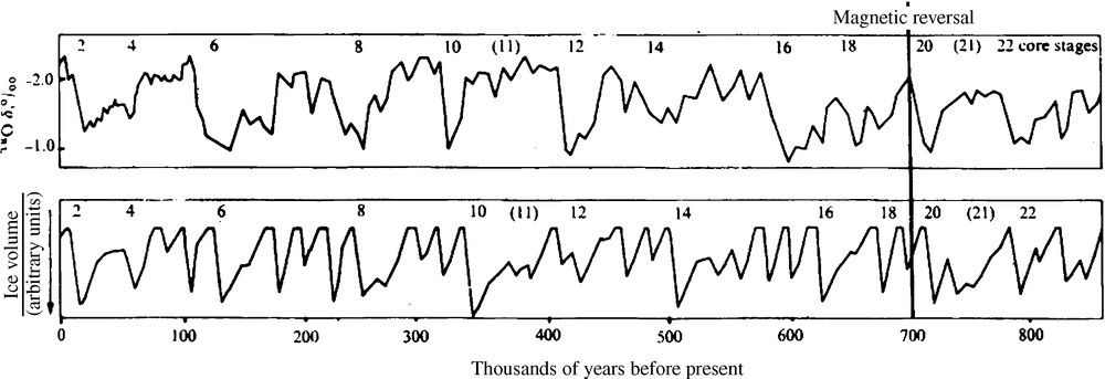
From Calder (1974) (Calder, 1974). Comparison between model results (below) and the isotopes in marine core V28-238 (Shackleton and Opdyke, 1973). Terminations are predicted at the correct time, while the chronology of the isotopic data is now known to be invalid (the Brunhes-Matuyama magnetic reversal is now estimated at 772 ka, and not 700 ka as on this figure). A posteriori, Calder's model made quite a remarkable prediction.
D’après Calder (1974) (Calder, 1974). Comparaison entre modèle (en bas) et isotopes marins de la carotte V28-238 (Shackleton and Opdyke, 1973). Les terminaisons sont prédites à des instants corrects, alors que la chronologie des données isotopiques est maintenant reconnue comme étant erronée (le renversement magnétique Brunhes-Matuyama est situé à environ 772 ka, et non pas 700 ka comme sur cette figure). A posteriori, le modèle de Calder a donc réalisé une prédiction assez remarquable.
But Calder's model is quite unstable and small changes in any of its two parameters (i0 or kA/kF) are leading to very different and unrealistic results. This is easily understood since the ice volume is basically the direct integral of insolation. Small changes in the threshold or in the coefficients are therefore rapidly amplified. A more robust model was formulated by Imbrie and Imbrie (1980) (Imbrie and Imbrie, 1980):
where V is now relaxed towards different values of VR depending on the climatic mode R in which the system stands. The model then switches from one mode to the other when some threshold is crossed, either for the insolation forcing i or for the ice volume V. This formulation allows a fundamental observation: in order to predict the right timing of the terminations, the climatic shift from a glacial state toward an interglacial regime must be triggered by a threshold on the ice volume. It is, by the way, for this same reason that Calder's model was so interesting: actually it predicts correctly the timing of the large glacial maxima which are in this model visually associated with terminations. In other words, terminations are caused in some unclear way by glacial maxima, rather than by the insolation forcing (Fig. 6).
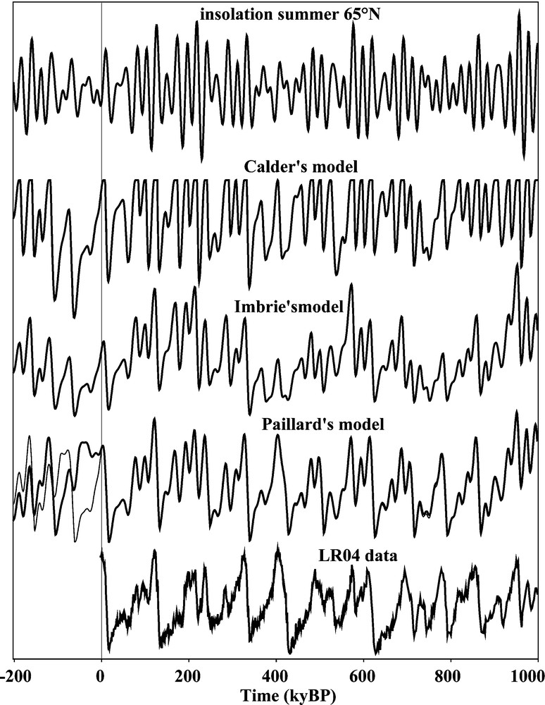
Comparison between the different simple models discussed here over the last million year and the next 200,000 years. From top to bottom: the daily insolation (65°N, june solstice) (Laskar et al., 1993), results from the Calder's model (Calder, 1974), the Imbrie's model (Imbrie and Imbrie, 1980), the Paillard's model (Paillard, 1998) and marine isotopic data (Lisiecki and Raymo, 2005). Note that in the threshold model (Paillard, 1998), there are two possible solutions for future glacial cycles, depending on threshold value (Paillard, 2001).
Comparaison entre les différents modèles simple mentionnés ici sur le dernier million d’années et les prochains 200 000 ans. De haut en bas : insolation journalière (65°N, solstice de juin) (Laskar et al., 1993), résultats du modèle de Calder (Calder, 1974), du modèle d’Imbrie (Imbrie and Imbrie, 1980), du modèle de Paillard (Paillard, 1998) et données isotopiques marines (Lisiecki and Raymo, 2005). Pour le modèle à seuil (Paillard, 1998), il existe deux solutions possibles pour les cycles futurs, en fonction des valeurs de seuil choisies (Paillard, 2001).
If the astronomical forcing is indeed at the source of the variability recorded during the Quaternary, the question of the climatic mechanisms involved remains largely unsolved. In the Milankovitch theory, the notion of “climate” is, in fact, simply reduced to the size of the ice-sheets in the northern hemisphere. Strictly speaking, the Milankovitch theory is a theory of ice sheet evolution, not a climate theory, as emphasized by the simple models above. If the astronomical forcing on the ice sheet has indeed some direct consequences on some aspects of Quaternary climate, it is clearly not sufficient, in particular to account for the largest cycles, that are occurring every 100,000 years. It is therefore necessary to complement this theory with a more mechanistic description of the climatic system involved, that is, larger than simply the ice sheet component.
5 Recent progresses
The analyses obtained from air bubbles trapped in Antarctic ice have clearly demonstrated that glacial–interglacial cycles are also associated with significant changes in the atmospheric concentration in CO2. This concentration changes from 180 ppm during glacial periods to 280 ppm during interglacial ones. These measurements are demonstrating that both historical theories on glacial ages, the astronomical one and the geochemical one, are actually valid. They are not exclusive from one another, but interact in some ways that still need to be understood. This was largely confirmed by the numerous climatic simulations of the last glacial maximum, which request a lowering of about 30 % of the atmospheric CO2 concentration in order to simulate a climate in broad agreement with the palaeoclimatic information. Furthermore, during terminations it is well established that the atmospheric CO2 concentration increases several millennia before the melting of the northern hemisphere ice sheets, as show on Fig. 7 by the sea level record of the last deglaciation. As shown on Fig. 4, if the Milankovitch theory accounts for most of the observed changes, this is no longer the case during terminations. It is therefore on those particular periods of time that we need to focus.
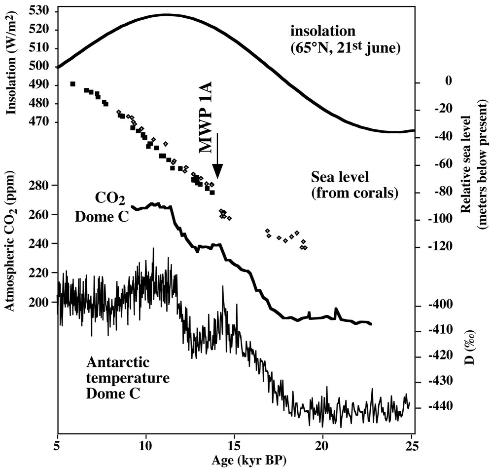
The last deglaciation. From top to bottom: the daily insolation (65°N, june solstice) (Laskar et al., 1993), the sea level record (Bard et al., 1996), the CO2 and temperature records from Dome C in Antarctica (Monnin et al., 2001). At about 15 kyrBP, while the sea level is still close to its glacial value (at about 100 m below present), the atmospheric CO2 has already risen by about 60 ppm from its glacial value, or more than half its full transition.
La dernière déglaciation. De haut en bas : insolation journalière (65°CN, solstice de juin) (Laskar et al., 1993), niveau marin (Bard et al., 1996), enregistrements de CO2 et de température à Dome C en Antarctique (Monnin et al., 2001). À environ 15 kyrBP, alors que le niveau marin est encore proche de sa valeur glaciaire (environ 100 m en dessous de l’actuel), le CO2 atmosphérique a déjà augmenté d’environ 60 ppm depuis sa valeur glaciaire, soit plus de la moitié de sa transition totale.
Glacial–interglacial changes are not limited to ice sheet changes that would then induce changes in the rest of the climate system. On the contrary, they result from a combination of ice sheet evolution, but also biogeochemical changes that are linked to climate in some way. The Milankovitch theory accounts only for one part of a more complex story. Unfortunately, our understanding of the carbon cycle during glacial times is very limited. Many hypotheses have been put forward to explain such lower CO2 levels during glacial periods, but none has yet succeeded in explaining a substantial part of the glacial interglacial 100 ppm difference. Actually, the situation is even worse, since the terrestrial biosphere was significantly reduced due to colder and drier climate on land, and the associated biospheric carbon needs also to be accounted for. Models using a closed carbon cycle between the atmosphere, the ocean and the terrestrial biosphere are thus generally predicting an increase in atmospheric CO2 in glacial conditions, because of the vegetation loss. The mechanisms that have been suggested so far are either based on physical and chemical changes in the ocean, or on changes in the biology and the corresponding biogeochemical cycles. Some authors have suggested that a complex combination of several of those different hypotheses, each one accounting for up to 10 or 20 ppm, may sum up to the right answer. But when looking at the palaeoclimatic records, the fantastic correlation between CO2 and the temperatures above Antarctica (Siegenthaler et al., 2005) is a strong indication that a rather direct link must exist between the climate of the Southern Ocean and CO2. This link is still largely missing.
However, recent progress is now accumulating. A first critical question raised by the models above is to better characterize glacial or interglacial “states”. Indeed, if ice ages are to be understood as a relaxation oscillation, then we need to define at least two different climatic regimes. The hypothesis of a strongly stratified deep ocean during glacial times, due to much saltier bottom waters, was put forward by Keeling and Stephens (Keeling and Stephens, 2001), then largely confirmed by pore water measurements from marine sediments by Adkins et al. (Adkins et al., 2002), but also by some model experiments (Stouffer and Manabe, 2003). The glacial ocean therefore appears quite different from the present day one, with a very strong stratification between the upper half and the lower half of the water column. These very salty bottom waters are likely to be formed around Antarctica through brine rejection during sea ice formation. Though the consequences of such an oceanic state onto the carbon cycle are still under investigation, it is likely that such a mechanism favors a strong storage of carbon in the deeper layers of the ocean, and thus an atmospheric CO2 decrease. With these assumptions, it is now possible to build a new simple model that can account more explicitly for the role of CO2 on glacial cycles (Paillard and Parrenin, 2004) as shown on Fig. 8.
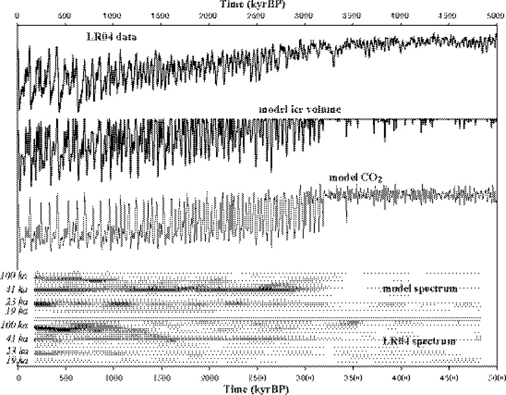
Model results from (Paillard and Parrenin, 2004) with a mechanism coupling the ice sheet evolution and the carbon cycle, forced by daily insolation (65°N, June solstice), and by a slow drift in a critical threshold parameter. The isotopic data (Lisiecki and Raymo, 2005) is shown at the top. Evolutive spectra on the bottom are showing the appearance of the 41 ka cyclicity about 3 million years ago, then the appearance of the 100 ka cyclicity about one million years ago, both in the model and in the data.
Résultats du modèle d’après (Paillard and Parrenin, 2004) incluant un mécanisme couplant l’évolution de la calotte de glace et le cycle du carbone, forcé par l’insolation journalière (65°N, solstice de juin), par une lente dérive d’un paramètre de seuil. Les données isotopiques (Lisiecki and Raymo, 2005) sont en dessous. Les analyses spectrales évolutives (en bas) montrent l’apparition de cycles à 41 ka il y a environ 3 millions d’années, puis l’apparition de cycles à 100 ka depuis un million d’années, pour le modèle comme pour les données.
In this model, terminations are explicitly induced by an increase in the model CO2, itself induced by the preceding glacial maximum, which destabilizes the oceanic deep stratification. This scenario leads to a reasonably good agreement between results and observations. Indeed, since it is based on a bimodal climatic system, it reproduces the features already found in (Paillard, 1998), like the possibility to switch the dominant frequency in the climatic response, from 23,000 years before the onset of glacial cycles in the Northern hemisphere, to 41,000 years between one and three million years ago, and to 100,000 year cycles during the last million years. Still, the mechanisms of these cycles need obviously to be described with detailed physical models, coupling the climate, the ice sheets and the carbon cycle. The time scales involved in this question is much too long to be addressed by state-of-the-art coupled ocean-atmosphere models, which are much too expensive in computing time (by at least 4 or 5 orders of magnitude). Furthermore, we also need to account for the ice sheet changes and for the major geochemical cycles. For these reasons, Earth models of intermediate complexity (or EMICs) are used increasingly to tackle such questions. The recent progress made both in palaeoclimatic reconstructions and in Earth's system modeling lets us envision, in the coming years, the building of renewed theory of ice ages. This new synthesis would account for the observational evidences and would also allow for satisfactory computer simulations of the largest climatic changes yet witnessed by homo sapiens.