Determination of flow exits in the Soultz borehole GPK2 by using the brine displacement method

Reinhard Jung; Marion Schindler; Patrick Nami; Torsten Tischner

doi:10.1016/j.crte.2009.06.002

Internal geophysics (Applied geophysics)

Determination of flow exits in the Soultz borehole GPK2 by using the brine displacement method
[Détermination des points de sortie du fluide dans le puits GPK2 par déplacement d’une saumure de remplissage]

Présenté par : Written on invitation of the Editorial Board

Reinhard Jung ¹ ; Marion Schindler ² ; Patrick Nami ³ ; Torsten Tischner ⁴

¹ Jung-Geotherm, Gottfried-Buhr-Weg 19, 30916 Isernhagen, Germany
² BESTEC GmbH, Oskar-von-Miller-Straße 2, 76829 Landau, Germany
³ Wintershall Holding AG, Friedrich-Ebert-Straße 160, 34119 Kassel, Germany
⁴ Federal Institute for Geosciences and Natural Resources (BGR), Stilleweg 2, 30655 Hannover, Germany

Comptes Rendus. Géoscience, Volume 342 (2010) no. 7-8, pp. 636-643.

Résumés

Anglais
Français

The article presents a method to derive synthetic flow logs from low rate injection tests in wells, which are otherwise not accessible for logging. The tests were carried out in the 5 km deep geothermal well GPK2 in the Enhanced Geothermal System (EGS) project of Soultz-sous-Forêts (France) and were aimed at characterizing the status of the well before chemical treatments. The method consists of injecting water at constant flow rates into the well initially filled with brine. The wellhead pressure record of this test is transformed into log of the flow velocity versus depth by a technique described in the paper. Applying this method to borehole GPK2, three outlets could be detected and quantified within the cased and uncased section of this borehole. The outlet in the cased section at 3860 m absorbed 15% of the total flow. This depth corresponds to a known casing restriction, which makes the borehole inaccessible for logging operations. The two other outlets are at the casing shoe at 4420 m (15%) and at 4670 m (70%).

Cet article présente une méthode permettant de calculer un profil de débitmétrie à partir des tests d’injection à faible débit dans les puits inaccessibles aux mesures. Les tests hydrauliques ont été effectués dans les trois puits géothermaux de 5000 m de profondeur, constituant le projet européen Enhanced Geothermal System (EGS) de Soultz-sous-Forêts (France). Les tests étaient destinés à caractériser les différents puits avant les opérations de stimulation chimiques. Lors de l’injection d’eau douce à faible débit dans des puits contenant de l’eau géothermale plus dense, il est possible de détecter les fuites à partir des mesures de pression en tête de puits. Par ce moyen, les profils de débitmétrie peuvent être calculés. Cet article présente le cas de GPK2, où trois fuites ont été détectées et quantifiées dans la partie tubée, ainsi que dans la section ouverte du puits. La fuite dans la partie tubée du puits, située à environ 3860 m, absorbe 15 % du débit total injecté. Cette profondeur correspond à une restriction déjà connue du tubage, empêchant toute accessibilité du puits aux mesures. Deux autres fuites ont également été détectées dans la section ouverte du puits : une au niveau du sabot du tubage à 4420 m (15 %) et l’autre à 4670 m (70 %).

Métadonnées

Reçu le : 2009-01-26
Accepté le : 2009-05-12
Publié le : 2009-09-03

DOI : 10.1016/j.crte.2009.06.002

Keywords: Hydraulic, Outlet zones, Flow log, Low rate injection, Soultz, EGS, HDR
Mot clés : Hydraulique, Zones de fuite, Profils de débitmétrie, Injection à faible débit, Soultz, EGS, HDR

Affiliations des auteurs :

Reinhard Jung ¹ ; Marion Schindler ² ; Patrick Nami ³ ; Torsten Tischner ⁴

¹ Jung-Geotherm, Gottfried-Buhr-Weg 19, 30916 Isernhagen, Germany
² BESTEC GmbH, Oskar-von-Miller-Straße 2, 76829 Landau, Germany
³ Wintershall Holding AG, Friedrich-Ebert-Straße 160, 34119 Kassel, Germany
⁴ Federal Institute for Geosciences and Natural Resources (BGR), Stilleweg 2, 30655 Hannover, Germany

@article{CRGEOS_2010__342_7-8_636_0,
     author = {Reinhard Jung and Marion Schindler and Patrick Nami and Torsten Tischner},
     title = {Determination of flow exits in the {Soultz} borehole {GPK2} by using the brine displacement method},
     journal = {Comptes Rendus. G\'eoscience},
     pages = {636--643},
     publisher = {Elsevier},
     volume = {342},
     number = {7-8},
     year = {2010},
     doi = {10.1016/j.crte.2009.06.002},
     language = {en},
}

TY  - JOUR
AU  - Reinhard Jung
AU  - Marion Schindler
AU  - Patrick Nami
AU  - Torsten Tischner
TI  - Determination of flow exits in the Soultz borehole GPK2 by using the brine displacement method
JO  - Comptes Rendus. Géoscience
PY  - 2010
SP  - 636
EP  - 643
VL  - 342
IS  - 7-8
PB  - Elsevier
DO  - 10.1016/j.crte.2009.06.002
LA  - en
ID  - CRGEOS_2010__342_7-8_636_0
ER  -

%0 Journal Article
%A Reinhard Jung
%A Marion Schindler
%A Patrick Nami
%A Torsten Tischner
%T Determination of flow exits in the Soultz borehole GPK2 by using the brine displacement method
%J Comptes Rendus. Géoscience
%D 2010
%P 636-643
%V 342
%N 7-8
%I Elsevier
%R 10.1016/j.crte.2009.06.002
%G en
%F CRGEOS_2010__342_7-8_636_0

Reinhard Jung; Marion Schindler; Patrick Nami; Torsten Tischner. Determination of flow exits in the Soultz borehole GPK2 by using the brine displacement method. Comptes Rendus. Géoscience, Volume 342 (2010) no. 7-8, pp. 636-643. doi : 10.1016/j.crte.2009.06.002. https://comptes-rendus.academie-sciences.fr/geoscience/articles/10.1016/j.crte.2009.06.002/

Version originale du texte intégral

1 Introduction

The European EGS (Enhanced Geothermal System; formerly called Hot Dry Rock) project Soultz is located in the Rhine Graben near Soultz-sous-Forêts in France, around 50 km north of Strasbourg, and investigates electricity production from hot deep crystalline rocks. Three 5000 m deep wells were successively drilled and hydraulically stimulated to activate the reservoir in the years between 2000 and 2004. The wells GPK2, GPK3, and GPK4 are aligned along the highest principal horizontal stress direction and give access to the formation in their uncased sections from 4500–5000 m depth where formation temperatures of 200 °C were encountered. Power production from these wells is achieved by circulating the geothermal water which is produced from the wells GPK2 and GPK4, extracting heat at the surface and reinjecting the cooled geothermal fluid in either GPK3 or an older well GPK1. In a first phase of power production, 1.5 MW_el are converted by an Organic Rankine Cycle (ORC) unit from geothermal flow rates between 30 and 35 l/s and temperature around 175 °C (Gérard et al., 2006; Tischner, 2006).

In 2006, the status of the wells GPK2, GPK3 and GPK4 was characterised prior to any further hydraulic stimulation or chemical treatment. The focus was to determine and quantify hydraulically active zones in the open hole sections and check the integrity of the wells (Pfender, 2006).

The most direct method to determine fluid outlets are flow logs recorded by impeller or spinner flowmeters which rotate proportional to the flow velocity. Other flowmeters base on tracer or thermal pulse methods whereas methods like temperature logs measure the temperature distortion caused by a permeable zone (Hearst et al., 2000). Many spinner and temperature flow measurements were successfully applied in the Soultz boreholes in the past (Tischner, 2006).

The status of GPK2 in March 2006 however was characterized by only one flow log, which was performed at the beginning of the massive hydraulic stimulation in July 2000. After this operation, a Pressure-Temperature-Flow (PTF) sonde with 700 m of cable remained in the well. The following inspection yielded a casing restriction (collapse) at around 3880 m where the wellbore is deviated (Fig. 1).

Fig. 1
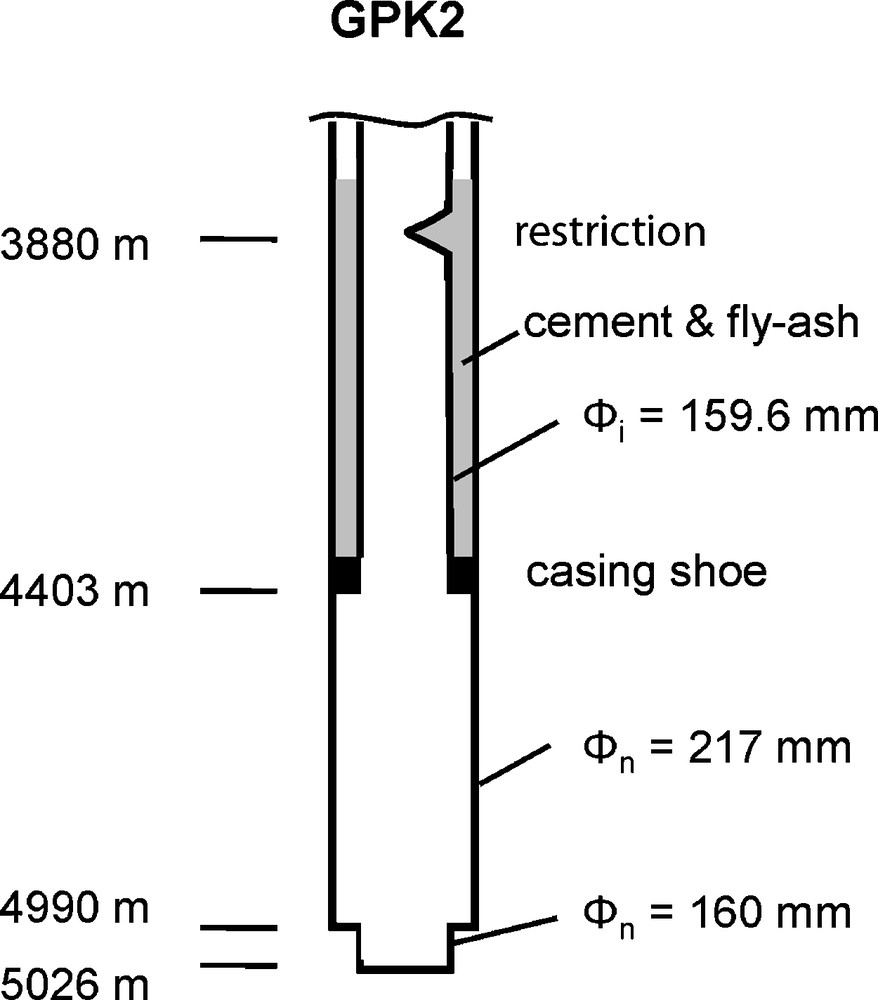
Scheme of the bottom part of borehole GPK2. Numbers on the left side: vertical depth; on right side Φ_i: internal diameter of the casing; Φ_n: nominal diameter of the borehole.
Schéma présentant la partie inférieure du puits GPK2. Sont indiqués à gauche: la profondeur verticale ; à droite : le diamètre interne du tubage Φ_i et le diamètre nominal du puits, Φ_n.

The well was not accessible below the restriction after this incident and no information about the outlets after stimulation was available. This information was missed the more since it was suspected that there might be a leak in the casing near the damaged zone. This question was of uttermost importance since such a leak might eventually connect the lower EGS-System with the shallower EGS-System created and tested in the previous project period.

For these reasons a new technique, which we call the brine displacement method was applied in the borehole GPK2. The method and the results obtained are described in the following sections.

2 The method

The method is based on the displacement of heavier brine filling a well by injecting lighter water. Assuming constant pressure at formation depth (steady state hydraulic conditions), the downward movement of the water-brine interface creates an increase of the wellhead pressure since the decreasing weight of the fluid column in the borehole has to be compensated by a corresponding increase of the wellhead pressure. This phenomenon is well known and was often observed during injection tests at Soultz. For constant flow rate the water–brine interface moves down with constant velocity and the wellhead pressure follows a linear trend. The velocity changes when the water–brine interface is entering a borehole section with different diameter, since fluid velocity and wellbore cross-sectional area are inversely correlated, and more important when it passes an outlet. Any velocity change is reflected by a corresponding change of the trend in the wellhead-pressure record (Fig. 2).

Fig. 2
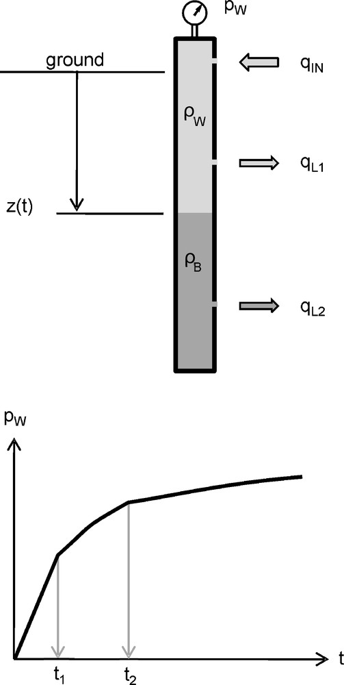
Illustration of the brine displacement method. ρ_W: density of water; ρ_B: density of brine; q_IN: injection flow rate; q_Li: flowrate lost at outlet i; z(t): vertical depth; t_i: time, when the water–brine interfaces reaches outlet i.
Illustration de la méthode de déplacement de la saumure par injection d’eau douce. ρ_W : densité de l’eau, ρ_B : densité de la saumure, q_IN : débit d’injection, q_Li : perte de débit à la sortie i, z(t): profondeur verticale, t_i: temps de passage de l’interface eau douce–saumure à la sortie i.

In practice, the wellhead pressure is not only affected by the downward movement of the water–brine interface but also by pressure transients resulting from the pressure build-up in the formation and from the cooling of the fluid column in the borehole (slow increase of the fluid density). The former creates a positive, the latter a negative trend.

Taking these effects into account, the following equations can be established which describe the wellhead pressure change relative to initial state as a function of time and depth of fluid interface:

p_{w} (z, t) - p_{w 0} = Δ p_{w} (z, t) = Δ ρ \cdot g \cdot z (t) + γ (t)

(1)

or

Δ p_{w} (z, t) = Δ p_{w}^{*} (z) + γ (t)

(2)

with: p_w: wellhead pressure;

p_{w 0} = p_{w} (z_{0}, t_{0})

: wellhead pressure at time t₀ when the water–brine interface is at a known depth z₀; t: time since start of injection; z(t): depth of the water–brine interface; Δρ: density difference between brine and water; g: Earth's acceleration due to gravity; γ(t): correction function.

This means the measured pressure $Δ p_{w} (z, t)$ , which is a function of the z and t, can be expressed as the sum of a function of z and a function of t.

The purpose of the next steps is to determine the function $Δ p_{w}^{*} (z)$ . For this aim we determine the first and the second derivative of $Δ p_{w} (z, t)$ with respect to time:

\frac{d}{d t} Δ p_{w} = \frac{d}{d t} Δ p_{w}^{*} + \frac{d}{d t} γ

(3)

\frac{d^{2}}{d t^{2}} Δ p_{w} = \frac{d^{2}}{d t^{2}} Δ p_{w}^{*} + \frac{d^{2}}{d t^{2}} γ

(4)

The term $\frac{d^{2}}{d t^{2}} γ$ can be determined by using pressure data from borehole sections where we know that the water–brine interface is moving at constant velocity. Here we can write:

\frac{d^{2}}{d t^{2}} z = 0

(5)

From this it follows:

\frac{d^{2}}{d t^{2}} Δ p_{w}^{*} = (\frac{d^{2}}{d t^{2}} Δ p_{w} - \frac{d^{2}}{d t^{2}} γ) = 0

(6)

or

\frac{d^{2}}{d t^{2}} γ = \frac{d^{2}}{d t^{2}} Δ p_{w} \approx φ (t)

(7)

$φ (t)$ is a fit-function fitting the data of $\frac{d^{2}}{d t^{2}} Δ p_{w}$ in those time intervals, where the velocity of the water–brine interface is known to be constant. By numerically integrating this function we get:

\frac{d}{d t} γ = \int_{t_{0}}^{t} φ (t) d t + c

(8)

with c: integration constant.

Inserting the right hand side of Eq. (8) in (3) yields:

\frac{d}{d t} Δ p_{w}^{*} = \frac{d}{d t} Δ p_{w} - \int_{t_{0}}^{t} φ (t) d t - c

(9)

The constant c is chosen so, that $\frac{d}{d t} Δ p_{w}^{*}$ at the end of the test is zero.

Numerical integration of $\frac{d}{d t} Δ p_{w}^{*}$ gives the corrected wellhead pressure-record we were looking for:

Δ p_{w}^{*} = \int_{t_{0}}^{t} (\frac{d}{d t} Δ p_{w}^{*}) d t

(10)

From this wellhead-pressure record the depth–time function of the water–brine interface can readily be determined:

z (t) = \frac{1}{Δ ρ \cdot g} \cdot Δ p_{w}^{*} + z_{0}

(11)

The derivative of this function gives the velocity of the water–brine interface:

v_{z} (t) = \frac{d z}{d t} = \frac{1}{Δ ρ \cdot g} \cdot \frac{d}{d t} Δ p_{w}^{*}

(12)

A cross-plot of $v_{z} (t)$ vs $z (t)$ gives the velocity of the water–brine interface as a function of depth. It should be noted that for both parameters (depth and velocity) the vertical components are meant. If a log of the borehole inclination is available, a log of the total velocity versus measured depth can be determined. The effect is minor as long as the borehole inclination is higher than 70̊ (as is widely the case in GPK2).

3 Test performance and results

A triplex piston plunger pump was deployed for injection. The injection rate was kept constant throughout the test at a value of 104 l/min ± 2 l/min. The density of the injection fluid was about 1.00 g/cm³ whereas the density of the brine was approximately 1.05 g/cm³. The wellhead pressure, flow rate and temperature of the injected water were recorded at sampling intervals of 1 s.

The records of the wellhead pressure and of the first and the second pressure derivative are shown on Fig. 3. The records start at a time t₀ = 200 min when the water–brine interface reached a depth of 504 m (bottom of the pumping chamber). It is clearly visible that the pressure has a negative trend and that the pressure derivative is negative toward the end of the test. This is obviously the effect of the cooling of the fluid column in the borehole due to injection, as mentioned in the previous chapter. A satisfactorily smooth curve of the first pressure derivative was obtained by averaging the pressure data over time intervals of about 8 min. For the smoothing of the second pressure derivative, pressure and its first derivative had to be averaged over about 40 min. This was acceptable since the time-dependent effects of temperature and of the pressure build-up in the formation are acting very slowly. Care was taken to use only pressure data from time intervals where the velocity of the water–brine interface was known to be constant. The fit-function approximating the data of the second pressure derivative is also shown on Fig. 3.

Fig. 3
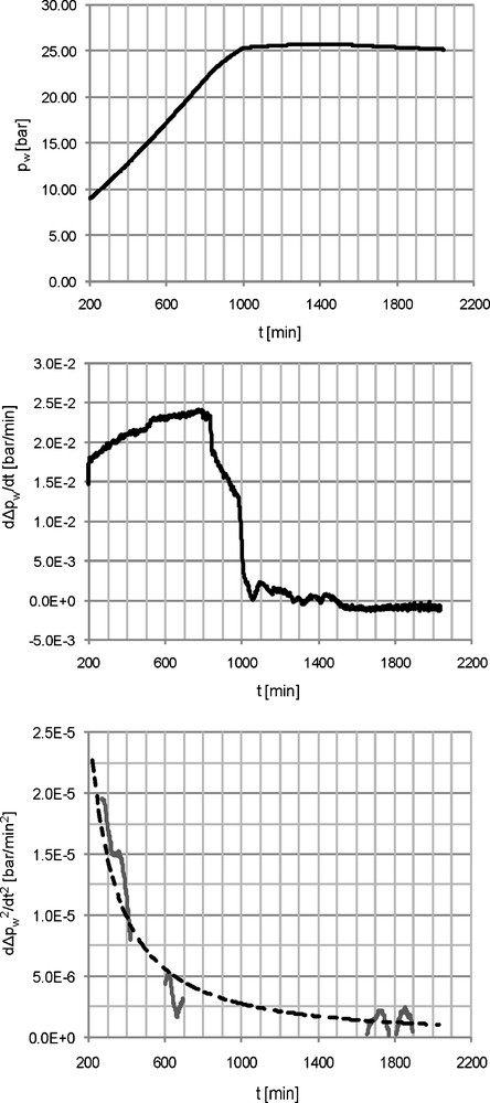
Top: wellhead pressure record; middle: first pressure derivative; bottom: second pressure derivative (line) and fitting curve (dashed line). t: time after start of injection. t = 200 min corresponds to the moment, when the water–brine interface reached the depth of 504 m (bottom of pumping chamber/top of 7”-casing).
En haut : mesures enregistrées de la pression en tête de puits. Au milieu : dérivée première de la pression (ligne continue). En bas : dérivée seconde de la pression (ligne interrompue). t : durée de l’injection. t = 200 min correspond au moment où l’interface eau douce–saumure atteint la profondeur de 504 m (profondeur de la chambre à pompe/tête du tubage 7”.

Fig. 4 shows the measured and corrected records of the pressure and its first derivative. The correction followed the procedure described in the previous chapter. The integration constant c (see previous chapter) was chosen so that the corrected pressure derivative toward the end of the test was zero. This presumes that the velocity of the water–brine interface is zero at the end of the test. A comprehensive analysis of the test results showed, that this is very likely the case.

Fig. 4
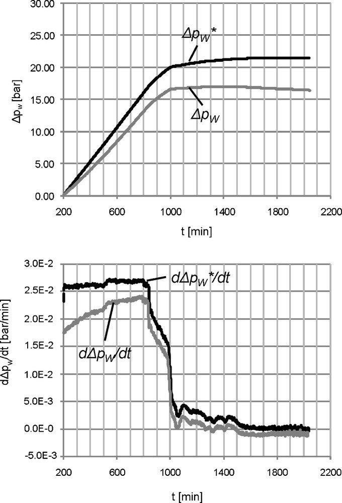
Top: measured and corrected pressure difference. Bottom: measured and corrected pressure derivative.
En haut : valeurs mesurées et corrigées de la différence de pression. En bas : valeurs mesurées et corrigées de la dérivée de la pression.

Figs. 5 and 6 show the vertical velocity of the water–brine interface as a function of the vertical depth. Vertical depth z(t) and velocity v_z(t) were determined from the corrected pressure record by using equations (11) and (12) of the previous section.

Fig. 5
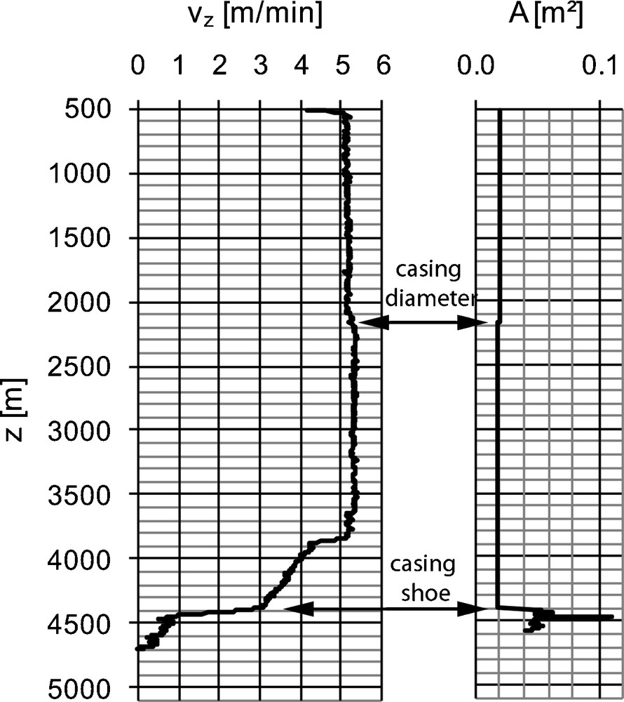
Velocity-log of the water–brine interface for borehole GPK2. Left: vertical velocity v_z of the water–brine interface; right: cross-sectional area of casing (< 4400 m depth) and openhole (> 4400 m depth); z: vertical depth. The velocity changes at about 2200 m and 4400 m are geometry-induced since borehole cross section and flow velocity are inversely correlated. The change in fluid velocity around 3860 m is independent of geometry.
Mesure de la vélocité de l’interface eau douce–saumure dans le puits GPK2. À gauche : vélocité verticale v_z de l’interface eau douce–saumure. À droite : section transversale du tubage (< 4400 m) et de la partie ouverte (> 4400 m) ; z: profondeur verticale. Les changements de la vitesse à 2200 m et 4400 m sont induits par la géométrie du tubage car la section transversale et la vélocité du fluide sont inversement en corrélation.

Fig. 6
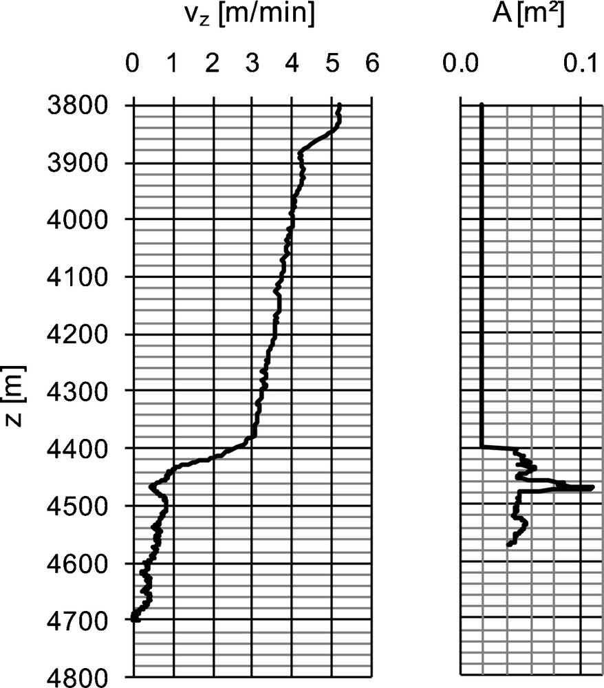
Velocity-log of the water–brine interface for the bottom part of borehole GPK2. Left: vertical velocity v_z of the water–brine interface; right: cross-sectional area of casing (< 4400 m depth) and openhole (> 4400 m depth); z: vertical depth. Note the minimum in v_z at 4470 m caused by the borehole enlargement at that depth.
Mesure de la vélocité de l’interface eau douce–saumure dans la partie inférieure du puits GPK2. À gauche : vélocité verticale v_z de l’interface eau douce–saumure. À droite : section transversale du tubage (< 4400 m) et de la partie ouverte (> 4400 m) ; z : profondeur verticale. Notez que le minimum en v_z à 4470 m est causé par l’agrandissement du diamètre du puits.

For this calculation, the density difference $Δ ρ$ between the injected freshwater and the brine has to be known precisely enough to yield an acceptable small depth error. For example, a density determined with an uncertainty of 1‰ causes an error in density difference of about 2% (density difference is about 0.05 g/cm³ in our experiment), which results in a depth uncertainty of 100 m at a 5000 m long well. Under the given experimental field conditions, an accuracy of 1‰ for the density measurement by aerometer could not be reliably achieved.

Therefore, instead of using the density values of water and brine as measured, z(t) and v_z(t) of equations (11) and (12) were determined with higher precision by calibrating the calculated depth–velocity diagram with known data points for the velocity and depth. One calibration point for the velocity is the top part of the casing where the fluid movement was known to be 5.2 m/min. Another, more precise calibration was performed by comparing the calculated velocity log to the caliper log of the openhole section, knowing that velocity correlates inversely to the cross-sectional area of the well. The marked enlargement of the cross-sectional area at 4470 m clearly correlates with a minimum in the flow-velocity log. Similarly, the small change in the cross-sectional area of the 7”-casing near 2200 m, caused by a casing weight change, corresponds well with a change in the velocity.

In contrast, the velocity decrease at about 3860 m is independent on geometry and therefore has to represent a fluid loss zone.

This remarkably good correlation between velocity-log and fixed data points highly validates the reliability of the velocity-log also in the other parts. For more quantitative evaluation it is better to use the flow log shown on Figs. 7 and 8. This was calculated from the velocity log by multiplying the velocity with the cross-sectional area given by the profile on Fig. 7.

Fig. 7
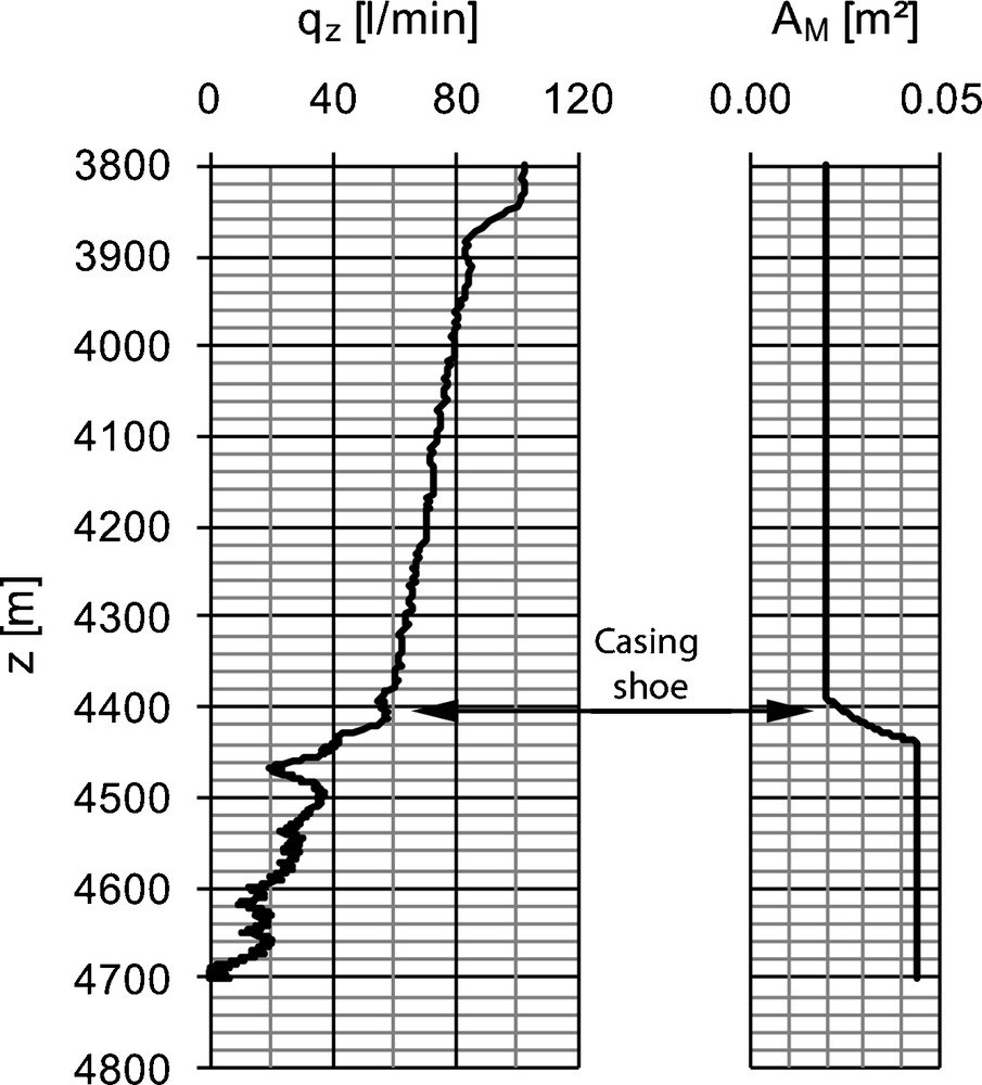
Flow-log of the bottom part of borehole GPK2. q_z: vertical component of the flow rate in borehole GPK2 (product of the vertical velocity of the brine–water interface from Fig. 6 with the cross-sectional area A_M).
Mesure de débimétrie de la partie inférieure du puits GPK2. q_z : composante verticale du débit dans le puits GPK2 (produit de la vitesse verticale de déplacement de l’interface eau douce–saumure de la Fig. 6 par la section transversale A_M).

Fig. 8
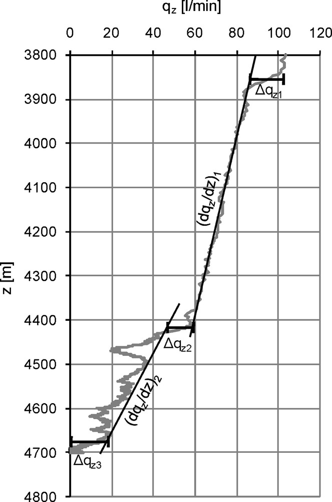
Flow-log of the bottom part of borehole GPK2 with lines and bars illustrating the readings of the parameters (dq_z/dz)_i and Δq_i.
Mesure de débimétrie de la partie inférieure du puits GPK2 : le diagramme en ligne et l’histogramme présentent les mesures respectives des paramètres (dq_z/dz)_i et Δq_i.

This presentation reduces the large step in the velocity log at the casing shoe where the cross-sectional area increases from 0.020 m² within the casing to 0.043 m² within the openhole. For the latter, a constant value was taken instead of the detailed log of the cross-sectional area as shown on Fig. 6. This was done since it was not possible to correlate the cross-sectional log with the velocity log in all details. The constant value of 0.043 m² is equal to the geometric mean of the measured average cross-sectional area and the nominal area and corresponds to an ellipse with the small axis equal to the nominal diameter of the well and the big axis equal to the diameter of a circle with the measured cross-sectional area. In order to avoid a peak of the flow at the casing shoe it was necessary to determine a transition profile of the cross-sectional area near the casing. This was found by trial and error. It affects the flow profile only in a narrow section at the transition between casing and openhole.

Three outlets can be identified on Figs. 7 and 8: One at 3860 m very close to the casing restriction, one near the casing shoe at about 4420 m, and one at 4680 m. A quantitative evaluation of these outlets is not an easy task since the loss rate at the different outlets is obviously changing after the water–brine interface has passed the uppermost outlet. Figs. 7 and 8 show clearly that after a sharp step at the uppermost outlet the flow is linearly decreasing with increasing depth of the water–brine interface. This effect is not surprising, since the fluid pressure at the uppermost outlet is linearly increasing with the depth of the water–brine interface after passing the outlet.

Two parameters of interest can directly be read from the diagram on Fig. 8. One is the step-like change of the flow $Δ q_{z i}$ . This parameter is identical with the lossrate at the outlet i. The other parameter is the derivative of the flow in the linear flow sections: ${(\frac{d q_{z}}{d z})}_{i}$ .

The values of these parameters are listed in Table 1.

Outlet number	Depth (m)	$Δ q_{z i}$ (l/min)	${(\frac{d q_{z}}{d z})}_{i}$ (l/(bar min))
1	3860	17	0.05
2	4420	13	0.113
3	4670	18	–

Total	–	–	–

From these parameters some interesting properties of the outlets can be determined:

The flow fraction lost at the outlet i (for i > 1) before the water–brine interface passes outlet 1 can be determined by:

\frac{q_{L i}}{q_{0}} = \frac{Δ_{q z i}}{q_{z (i - 1)}} \cdot \prod_{n = 1}^{i - 1} (1 - \frac{Δ q_{q_{n}}}{q_{z (n - 1)}})

(13)

with $q_{z i}$ : value of the flow rate immediately above outlet i. The injectivity index of the two upper outlets is given by:

I I_{1} = \frac{1}{g \cdot Δ ρ} {(\frac{d q_{z}}{d z})}_{1}

(14)

I I_{2} = \frac{1}{g \cdot Δ ρ} ({(\frac{d q_{z}}{d z})}_{2} - {(\frac{d q_{z}}{d z})}_{1})

(15)

The values determined with these equations are listed in Table 2.

Outlet number	Depth (m)	(q_i/q₀)_i (%)	II_i (l/(bar min))	Δp (bar)
1	3860	16	10	1.7
2	4420	18	12	1.7
3	4670	66	38	1.7

Total		100	60	1.7

The value of the hydraulic pressure build-up at the time when the water–brine interface reaches the uppermost outlet is given by:

Δ p = \frac{Δ q_{z i}}{I I_{1}}

(16)

The total injectivity index of the borehole is given by:

I I_{t} = \frac{q_{0}}{Δ p}

(17)

and is also listed in Table 2.

The values of the injectivity determined from the slope of the flow log and the values of the flow fraction derived from the step-like flow change in the flow log agree quite well.

In summary, we can conclude that for steady state conditions (before the water–brine interface passed the uppermost outlet) about 15% of the flow was lost at each of the two higher outlets at 3860 m and 4420 m and that the majority of the flow (70%) was lost at a structure at 4670 m.

4 Summary and conclusions

4.1 Methodology

A new method was developed to determine flow velocity logs in boreholes not accessible by logging sondes. This method consists of injecting water in a borehole previously filled with brine. The wellhead pressure–time record is transformed into a flow-velocity-log by using a technique described in the previous sections. If at least one calibration point (depth or velocity) is available this transformation can be done without knowing the fluid-density difference between water and brine and without knowing the exact flow rate. Both can be determined from the calibration. The only assumption is that the density-difference and the flow rate are constant throughout the test. The resolution of the method is in the order of 0.1 m/min. The interpretation of the flow velocity log obtained with this new method however is complex, since the flow distribution to the different outlets is changing after the water–brine interface has passed the uppermost outlet. This is an intrinsic problem of the method that could possibly be solved by performing several tests with different flow rates or fluid densities. This could also solve the potential problem of not reaching the lowermost outlets with the water–brine interface due to the increasing fluid losses at the upper outlets when the water–brine interface moves downward.

4.2 Application in GPK2

Three outlets were localized and quantified by applying the brine displacement method in borehole GPK2:

The uppermost outlet is near the casing damage at 3860 m. This outlet absorbed about 15% of the total flow before the water–brine interface passed this depth. The loss rate at this outlet increased linearly with the depth of the water–brine interface afterwards. This indicates that the outlet reacts almost instantaneously to the changing pressure conditions. It can therefore be suspected that a small leak in the casing and not the structure (joint or fault) linked with this leak is controlling the loss rate. The casing damage is situated at about 160 m below the top filler (≈ 3740 m) and 10 m below a cave. An abnormal trend of the annulus pressure was not observed during the test, indicating that the casing restriction is not hydraulically connected to the annulus of GPK2.

Another outlet also absorbing about 15% of the total flow is observed well below the casing shoe at 4420 m. The loss rate at this outlet also increased with increasing depth of the water–brine interface after this had passed the outlet. This is reflected by a steeper decrease of the flow velocity below the depth of this outlet.

The majority of the flow (about 70%) leaves at an outlet at about 4670 m. Due to the very small velocity of the water–brine interface at this depth this outlet is hardly visible in the velocity log, and even in the flow log where the flow in this section is exaggerated this outlet is not very pronounced. This shows that the velocity and flow logs obtained by the brine-displacement method have carefully be analyzed to get reliable results. This applies especially to the deeper part of these logs.

Acknowledgements

The work was part of the Hot-Dry-Rock-Project Soultz, funded by GEIE, ADEME and BMU. We thank all GEIE personal for the successful realization of the test. MeSy greatly contributed with technical assistance. We would like to thank the Bestec and LIAG personnel for their participation and support in the framework of these tests.

Bibliographie

[Gérard et al., 2006] A. Gérard; A. Genter; T. Kohl; P. Lutz; P. Rose; F. Rummel The deep EGS (Enhanced Geothermal System) project in Soultz-sous-Forêts (Alsace, France), Geothermics, Volume 35 (2006), pp. 473-483

[Hearst et al., 2000] J.R. Hearst; P.H. Nelson; F.L. Paillet Well logging for physical properties, John Wiley and Sons, Ltd, New York, 2000 (483 p)

[Pfender, 2006] Pfender, M., Nami, P., Tischner, T., Jung, R, 2006. Status of the Soultz deep wells based on low rate hydraulic tests and temperature logs, EHDRA Scientific Conference, 15.-16.06.2006, Soultz-sous-Forêts, France, pp. 1–12 (Proceedings).

[Tischner, 2006] Tischner, T., Pfender, M., Teza, D, 2006. Hot Dry Rock Projekt Soultz: Erste Phase der Erstellung einer wissenschaftlichen Pilotanlage, Final project report.

Commentaires - Politique