

1 The need for global observation of the ozone layer
The depletion of the stratospheric ozone layer was the first environmental issue that aroused international concerns on the possible impact of human activities on the Earth's atmosphere at a global scale. While ozone abundance is very small in the atmosphere, not exceeding 8 to 10 molecules per million air molecules, its role on the equilibrium of the atmosphere and life on Earth makes it one of the key species in the atmosphere. Ozone absorbs ultraviolet (UV) radiation from the incident solar light. Much of the absorbed energy is input into the atmosphere and is responsible for the temperature inversion in the stratosphere, an atmospheric region that extends from about 12 to 50 km altitude. The other remarkable property of ozone is that it shields the Earth's surface from damaging UV-B radiation (280–320 nm spectral range) due to its spectroscopic properties. Before there was ozone, life was restricted to marine environments and it was only after the ozone layer was formed, about two billion years ago, that life could expand at the surface. While ozone is beneficial when it exists at high altitude, its oxidizing properties makes it harmful to human health when it is produced as a pollutant close to the surface, where it can also affect animals and plants.
Since the 1970s, as their understanding of the ozone equilibrium in the atmosphere grew, scientists raised concerns about the potential threat to the ozone layer caused by increased emission of human-manufactured chlorofluorocarbons (CFC) and halons. However, the major event was the discovery of the ozone hole over Antarctica (e.g. Chubachi, 1984; Farman et al., 1985). Although satellite measurements were not at the origin of this discovery, made from ground-based Dobson spectrometer and balloon-borne ozone sonde measurements, they played an important role on the quantification of the spatial extent of the chemical ozone destruction over Antarctic. Indeed, after the Farman et al. publication, satellite measurements showed that in each late winter/early spring season starting in the early 1980s, the ozone depletion extended over a large region centered near the South Pole. The term “ozone hole” came about from satellite images.
Since then, spatial ozone measurements have been widely used to evaluate and quantify the spatial extension of the ozone hole and global ozone decreasing trends as a function of latitude and height. Validation and evaluation of satellite ozone data have been the subject of intense scientific activity, which has been reported in the various ozone assessments of the state of the ozone layer published after the signature of the Montreal protocol. This article provides an overview of the various satellite instruments, which were developed for the observation of ozone and chemical compounds playing a key role in stratospheric chemistry. It describes the instruments that have been launched since the late 1970s for the measurement of the total ozone column and vertical distribution, as well as the major satellite missions designed for the study of stratospheric chemistry. Major satellite instruments are listed in Table 1. The main results, based on satellite observations for the study of ozone depletion at global scale and chemical polar ozone loss, are provided. The use of satellite observations for the validation of atmospheric models and data assimilation is also described.
Principaux instruments satellitaires mis en œuvre pour l’étude de la couche d’ozone.
| Instrument | Satellite | Operating period | Main measured species |
| BUV | Nimbus-4 | 1970–1980 | O3 (total column) |
| SBUV | Nimbus-7 | 1978–1985 | O3 (total column, vertical profile) |
| SBUV-2 | NOAA series | 1986–1988 | O3 (total column, vertical profile) |
| TOMS | Nimbus-7 Meteor-3 ADEOS EarthProbe |
1978–1992 1991–1994 1996–1997 1996–2006 |
O3 (total column) |
| OMI | Aura | 2004– | O3, NO2, SO2, BrO, OClO, aer |
| GOME | ERS-2 | 1995– | O3, NO2 |
| LIMS | Nimbus-7 | 1978–1979 | O3, H2O, HNO3, NO2 |
| SAGE | AEM-B | 1978–1982 | O3, aer |
| SAGE II | ERBS | 1984–2005 | O3, NO2, H2O, aer |
| HALOE | UARS | 1991–2005 | O3, NO2, H2O, aer |
| MLS | UARS Aura |
1991–2001 2004– |
O3, H2O, HNO3, N2O, ClO O3, H2O, HNO3, N2O, ClO |
| ISAMS | UARS | 1991–1992 | O3, H2O, CH4, CO, NOy, aer |
| CLAES | UARS | 1991–1992 | O3, H2O, HNO3, N2O, ClO |
| POAM II | Spot-3 | 1993–1996 | O3, NO2, H2O, aer |
| POAM III | Spot-4 | 1998–2006 | O3, NO2, H2O, aer |
| ODIN | START-1 | 2001– | O3, ClO, N2O, CO, H2O |
| ILAS | ADEOS | 1996 | O3, H2O, HNO3, NO2, N2O, CH4, aer, CFC-11 |
| ILAS II | ADEOS-II | 2003 | O3, H2O, HNO3, NO2, N2O, CH4, aer, CFC-11 |
| GOMOS | Envisat | 2002– | O3, NO2, H2O, aer |
| MIPAS | Envisat | 2002– | O3, H2O, HNO3, N2O, CH4, aer |
| SCIAMACHY | Envisat | 2002– | O3, NO2, BrO, SO2, OClO, H2O |
| HIRDLS | Aura | 2004– | O3, HNO3, CFC-11, CFC-12, aer |
| ACE-FTS | SCISAT-1 | 2003– | O3, HNO3, N2O, H2O, CH4, aer |
| MAESTRO | SCISAT-1 | 2003– | O3, NO2, H2O, OClO, BrO |
| IASI | METOP | 2006– | O3, CO, CH4, N2O |
| GOME 2 | METOP | 2006– | O3, NO2 |
2 Total ozone column observation from space
2.1 Satellite instruments for the measurement of total ozone column
A convenient way to measure ozone abundance is to measure its total column, which corresponds to the total number of ozone molecules in a column from the Earth's surface to the top of the atmosphere. It is generally expressed in Dobson units1. From the various satellite instruments that measure the total ozone column, probably the most famous is the Total Ozone Mapping Spectrometer (TOMS) that has been operated by the National Aeronautic and Space Administration (NASA) from 1978 until 2006. TOMS measures solar ultraviolet radiation scattered back into space by air molecules. Total ozone is retrieved from the different absorption of solar radiation by ozone at various wavelengths in the UV range. The first TOMS instrument began operation on board the Nimbus 7 meteorological satellite, which included also the Solar Backscatter Ultraviolet (SBUV) instrument, another ozone-measuring sensor. TOMS looked downward at several angles across the nadir track of the satellite to measure backscattered radiation at six wavelengths ranging from 312 to 380 nm. SBUV was designed to measure the ozone vertical distribution and total ozone. It looked in the nadir direction and measured the backscattered radiation at 12 wavelengths ranging from 250 to 400 nm. The concept of these instruments was based on the original Backscatter Ultraviolet (BUV) launched in 1970. The SBUV and TOMS instruments on board Nimbus 7 continued to make measurements until 1990 and 1994, respectively. The SBUV was followed by the series of SBUV/2 instruments launched on the NOAA polar orbiting series. The TOMS instrument was followed by Meteor TOMS on the Russian Meteor 3 satellite and the Earth Probe TOMS, which operated up to 2006 (see Fig. 1). The TOMS total ozone record has been taken over by the Ozone Monitoring Instrument (OMI), launched on the Aura satellite in 2004. OMI is the result of a Dutch /Finnish /American collaboration. It uses hyperspectral imaging in the visible and ultraviolet range for the retrieval of ozone and key air quality components such as NO2, SO2, BrO, OClO, and aerosol characteristics. OMI makes cross-track measurements like TOMS, but with an improved spatial resolution. It has also the capability to retrieve the ozone profile, like the SBUV instruments.

Merged total ozone data set from SBUV and TOMS instruments updated through late 2007. The series of satellite instruments used to construct the series is shown in the top panel. Monthly-mean area-weighted averages over the latitude range from 60°S to 60°N are shown in the bottom panel (Stolarski and Frith, 2006).
Séries temporelles d’ozone, fusionnées à partir des mesures SBUV et TOMS jusqu’en 2007. Panneau du haut : instruments satellitaires utilisés pour la construction des séries temporelles ; panneau du bas : moyennes mensuelles pondérées par la surface dans la région de latitudes comprises entre 60 °S et 60 °N (Stolarski et Frith, 2006).
Another important instrument to measure total ozone is the Global Ozone Monitoring Experiment (GOME) instrument, which was launched on board the European Space Agency's ERS-2 satellite in April 1995. It was the first European experiment dedicated to global ozone measurements (Burrows et al., 1999). GOME has been operational since June 1995, but spatial coverage has been limited since July 2003 due to problems with tape storage on ERS-2. GOME measures the backscattered radiance from 240–790 nm in the nadir-viewing geometry. The maximum scan width in the nadir is 960 km across track on the ground and global coverage is completed within three days. Various algorithms based on the Differential Optical Absorption Spectroscopy (DOAS) technique were developed for GOME applications and used to reprocess the GOME total ozone data. For all the algorithms, the GOME total ozone data retrieved show excellent agreement with each other and with ground-based Brewer and Dobson measurements at mid-latitudes (WMO, 2007).
Column ozone can also be determined by measuring the thermal radiation emitted by ozone molecules in the atmosphere. Such observations are made by the TIROS Operation Vertical Sounder (TOVS). The TOVS data are retrieved using radiance measurements made by the High Resolution Infrared Sounder (HIRS) at 9.7 μm. Unlike the ultraviolet-based instruments, TOVS can measure into the polar night. However, the retrieval technique is sensitive to ozone changes between 4 to 23 km altitude only. The accuracy of the total ozone estimate is therefore compromised when ozone changes occur in the mid-to-upper stratosphere (Miller, 1989).
2.2 Validation and merging of total ozone satellite observations
While providing a quasi-global coverage of the ozone field, satellite measurements require to be validated against ground-based observations after the launch and during the whole operation of the instruments, since they generally show degradation over time. Ground-based networks like the Global Atmospheric Watch (GAW), Dobson and Brewer networks or the Network for the Detection of Atmospheric Changes instruments (http://www.ndacc.org) are used to check the long-term drift of satellite observations. Such an exercise is regularly performed in order to check the homogeneity of satellite records and new versions of the retrieval algorithms are periodically released in order to correct possible biases in the time series. The initial TOMS algorithm yielded ozone time series with declining trends much larger than those retrieved from the ground-based observations (WMO 1990). It was then recognized that much of this trend was due to the degradation of the diffuser plate used to reflect direct solar radiation into the instrument. A method was devised to correct the drift (Herman et al., 1991) and the TOMS measurements could be used along with ground-based records to provide first estimates of ozone trends (WMO, 1990).
In order to detect ozone trends of a few percents per decade, a large effort has been made in order to improve the accuracy of the various ground-based and satellite ozone-monitoring systems. Validation studies have shown that satellite measurements can be used as a transfer standard among ground-based stations. A change relative to satellite observations seen at one station can be attributed to a problem at that station, while a change relative to many stations is more likely to be caused by a problem in the satellite instrument. Such a strategy was applied by (Fioletov et al., 1999) to check the performance of the ground-based total ozone network performance. The latest comparison of column ozone datasets shows that the best agreement between ground-based and satellite data is found over northern mid-latitude. In that region both data sets agree within to 1%, while there is a 2–3% systematic difference over tropical and equatorial regions and over southern mid-latitudes. At high latitude in both hemispheres, differences increase and can reach 5–10% over the Antarctic. However, the differences among the data sets are generally much smaller than the observed natural short-term ozone variations as well as the long-term decline of global total ozone amount (WMO, 2007). The need for long data records such as total ozone time series requires the merging of measurements from several satellite instruments. Several times series have been created for the evaluation of ozone evolution at a global scale. One example is the merged TOMS + SBUV/2 dataset (Stolarski and Frith, 2006). An external calibration adjustment is applied to each record in an effort to calibrate all the instruments to a common standard. Such data sets have been used in the latest ozone assessments to analyse the temporal evolution of ozone at various spatial and temporal scales (see section 5).
3 Ozone profile measurements
The ozone vertical distribution can be measured from space by a variety of techniques that include nadir sounding in various parts of the solar radiation spectrum, solar occultation, limb scattered light and limb emission measurements. Solar and stellar occultation measurements are made by measuring radiation from the sun or a star as they set or rise. During these transitions, the instrument views the source through the atmosphere and the radiation is attenuated by scattering and absorption by minor constituents. Measurements made above the Earth's atmosphere are not attenuated and these data can be used to calibrate the instrument response. The fundamental measurement made by such instruments is a spectral slant path atmospheric transmission profile. These transmission profiles are then analysed in order to infer aerosol extinction and species density profiles of species like ozone, NO2, and H2O as a function of altitude. This technique provides high vertical resolution (∼1 km) and very small long-term drifts resulting from instrument calibration. However, spatial sampling is limited, and it takes approximately one month to sample the 60°N to 60°S latitude range in the case of solar occultation. This technique has been used by a variety of instruments such as SAGE I and SAGE II developed by NASA, HALOE on board the Upper Atmosphere Research Satellite (UARS) launched in 1991, and the series of Polar Ozone and Aerosol Measurement (POAM) instruments developed by the Naval Research Laboratory (NRL). Launched on board the Earth Radiation Budget Satellite (ERBS), the SAGE II instrument has provided the longest global ozone profile record, from 1984 to 2005. Comparisons with ground-based measurements showed that the quality of the latest version of SAGE II ozone profiles is excellent down to the tropopause, except after the eruption of Mt. Pinatubo in June 1991 when aerosol interference contaminated the measurements at the altitude of the volcanic aerosol cloud (Gleason et al., 1993). The HALOE instrument provided also a long ozone data record of about 14 years between 1991 and 2005. The POAM II was launched aboard the French SPOT-3 satellite in 1993 into a Sun synchronous polar orbit. The measurements were made at latitudes larger then 55°N and 63°S, which allowed them to be used for the study of the ozone loss in the Polar Regions. POAM II was followed by POAM III launched on board SPOT-4 in 1998. It operated until 2006. The Global Ozone Monitoring by Occultation of Stars (GOMOS) instrument was launched onboard the Envisat satellite in 2002 and is operated by the European Space Agency since then. It uses the stellar occultation technique and provides a global record of ozone profiles and other atmospheric compounds such as NO2 and H2O. The most recent satellite mission using the solar occultation technique is the Canadian Atmospheric Chemistry Experiment satellite launched in 2003. It includes two instruments, ACE-FTS a high spectral resolution infrared Fourier Transform Spectrometer (FTS), and a UV-visible-Near Infrared spectrophotometer known as MAESTRO.
A technique somewhat similar to the occultation technique is to observe the limb (edge) of the Earth's atmosphere. The Microwave Limb Sounder (MLS) experiments developed by the Jet Propulsion Laboratory (JPL) use this method to remotely sense vertical profiles of atmospheric gases, temperature, pressure, and cloud ice. The first MLS experiment was launched on the NASA UARS platform in 1991 and ceased operation in 2001. The second one (EOS MLS) is on the NASA Earth Observing System (EOS) Aura mission launched in 2004. Along with ozone it measures other important species involved in stratospheric chemistry such as H2O, HNO3, N2O and ClO.
Nadir sounding instruments providing total ozone measurements such as SBUV and GOME can also provide information on the ozone vertical distribution. Both instruments measure in the near ultraviolet where ozone absorption is strong and change rapidly with wavelength. Rayleigh scattering2 is also stronger towards shorter wavelengths and as atmospheric density increases. These effects provide a scanning function whereby shorter UV wavelengths are more strongly affected by the absorption of ozone at higher altitudes (e.g. Bhartia et al., 1996). The general problem of inverting nadir backscatter measurements to derive an ozone profile is ill-conditioned. One must apply some sort of constraint to achieve a physically reasonable solution. The most common way is to apply the optimal estimation method, which derives ozone by selecting a profile that has the highest probability of being the correct profile, based on a priori statistical information (Rodgers, 1990). Nadir sounding instruments provide a much better coverage of the ozone field than the occultation technique, but at the expense of a much lower resolution of the retrieved ozone profiles (several kilometres).
4 Main satellite missions dedicated to stratospheric chemistry
The full understanding of the various causes of ozone decrease at the global scale requires accurate long-term measurements of not just ozone but also a broad range of chemical species and long-lived tracers that influence the ozone budget in the stratosphere. To that aim several major atmospheric missions have been launched since the early 1980 s. A first insight of the atmospheric composition in the stratosphere was provided by the Limb Infrared Monitor of the Stratosphere (LIMS), which operated on board Nimbus 7 for several months in 1978/79 and by the Spacelab 3 Atmospheric Trace Molecule Spectroscopy (ATMOS) carried on the Space Shuttle in 1985. In 1991, a major satellite mission dedicated to stratospheric chemistry was launched: the Upper Atmospheric Research Satellite (UARS, Reber, 1993). UARS included several instruments for the measurements of stratospheric compounds: MLS, HALOE, the Improved Stratospheric and Mesospheric Sounder (ISAMS) and the Cryogenic Limb Array Etalon Spectrometer (CLAES), the two latter instruments both working in the infrared. UARS also measured winds and temperatures in the stratosphere as well as the energy input from the Sun. In addition to providing the first comprehensive picture of the atmospheric composition in the stratosphere, one of the major results of the UARS mission was the evaluation of chlorine activation in the Polar Regions. MLS measurements of chlorine monoxide (ClO) showed that chlorine in the lower atmosphere was almost completely converted to chemically reactive forms in both southern and northern polar vortices in winter, before the start of chemical ozone depletion (Waters et al., 1993). Fig. 2 shows enhanced ClO together with depleted ozone amounts in the southern polar vortex, as measured by MLS in 1991.

ClO and O3 in the Southern Hemisphere as measured by MLS UARS at around 18 km in September 1991 (Waters et al., 1993).
Champs de monoxyde de chlore et d’ozone dans l’Hémisphère Sud mesurés par MLS à bord d’UARS vers 18 km en septembre 1991 (Waters et al., 1993).
The ESA's Environmental Satellite (Envisat) was launched in 2002 with three instruments dedicated to atmospheric chemistry: GOMOS (described in section 3), the Michelson Interferometer for Passive Atmospheric Sounding (MIPAS) and the Scanning Imaging Absorption spectrometer for Atmospheric CHartographY (SCIAMACHY). MIPAS is a Fourier transform spectrometer operating in the near to mid infrared for the measurement of high-resolution gaseous emission spectra at the Earth's limb. SCIAMACHY is an imaging spectrometer, which aims at performing global measurements of trace gases in the troposphere and stratosphere. It has three different viewing geometries: nadir, limb, and sun/moon occultation, which yield total column values as well as distribution profiles in the stratosphere and (in some cases) the troposphere. These three instruments have provided since 2002 comprehensive data sets of stratospheric species, which were used for the study of ozone depletion in Polar Regions or the ozone budget in other atmospheric regions. The Envisat atmospheric composition data strongly contribute to assimilation systems such as those participating to the ESA PROMOTE project (http://www.gse-promote.org) in various areas (stratospheric ozone, air quality, UV monitoring and climate).
Aura, the last of the large Earth Observing System observatories, was launched by NASA in 2004. Aura was designed to make comprehensive stratospheric and tropospheric composition measurements from its four instruments, the High Resolution Dynamics Limb Sounder (HIRDLS), the Microwave Limb Sounder (MLS), the Ozone Monitoring Instrument (OMI), and the Tropospheric Emission Spectrometer (TES). As far as the ozone layer is concerned, one of the results of Aura was to show that HCl (measured by MLS) has started to decline in the upper stratosphere with a rate consistent with surface abundance decrease rates in chlorine source gases, taking into account a delay of about 6 years (Froidevaux et al., 2006). This result corroborates the success of the Montreal Protocol with respect to the cleansing of the stratosphere of the excess of chlorine loading due to human activities.
In addition to these three major satellite missions, one can also cite the ODIN satellite launched in 2001 as a result of Swedish, Finish, Canadian and French cooperation, and the ADEOS I and II satellites launched by Japan's National Space Development Agency. However, both ADEOS satellites were lost after less than one-year operation.
5 Temporal evolution of the ozone layer at global scale
5.1 Total ozone trend estimation
Expected changes in the ozone layer prompted statistical studies of available ozone records in an attempt to detect long-term trends. The first satellite estimates of total ozone trends were made by (WMO, 1990) using Nimbus-7 TOMS data over the 1979–1989 period. After recalibration of the satellite data using ground-based measurements, the reported accumulated ozone loss was estimated to range from 1.2 to 2.7% in the northern mid-latitudes. Since then, the successive assessments on the state of the ozone layer have quantified the decline of the ozone layer using the various ozone records. Fig. 3 shows the latest estimate of total ozone deviations for the 90°S–90°N and 60°S–60°N latitude belts, from various ground-based, satellite and merged data sets (WMO, 2007). Each dataset was deseasonalized and the deviations were expressed as percentages of the ground-based time average for the period 1964–1980. Top and bottom plots show seasonal and yearly averages, respectively. The ozone deviations in the most recent years show a stabilisation of the decline of the ozone layer at global scale since the early 2000 s. The main periodic components in the temporal evolution of ozone are the 11-year solar cycle and the Quasi-biennal Oscillation (QBO)3, which has a period of 2–3 years. Another distinctive feature is the ozone depletion due to the high stratospheric aerosol loading originated from the Mount Pinatubo eruption in 1991 (Gleason et al., 1993). This decrease was linked to the chemical activation of chlorine compounds, caused by processes similar to those occurring in the Polar Regions in winter. The depletion lasted for 2–3 years after the eruption and was modulated by temperature conditions in the winter stratosphere (WMO, 1998). It was estimated that global mean total column ozone values for the period 2002–2005 were approximately 3.5% below the 1964–1980 average values. They were similar to the 1998–2001 values, indicating that ozone is no longer decreasing (WMO, 2007).
5.2 Trends in the vertical distribution of ozone
In order to estimate long-term changes of ozone at a global scale as a function of altitude one has to use the longest satellite records of the ozone vertical distribution. The most recent ozone assessment used the SAGE I + II and SBUV ozone records and compared them with ground-based measurements from ozone sondes and Dobson spectrometer (see Fig. 4). The ozone vertical distribution can be retrieved from Dobson spectrometer measurements during sunrise and sunset, using the Umkehr method (e.g. Mateer and Deluisi, 1992). The vertical profile of ozone trends reflects the influence of halogen compounds on ozone as a function of altitude. This influence is largest in the upper and lower stratosphere. Around 40 km, the ozone loss is due to catalytic cycles involving chlorine radicals, while at 20 km it is caused by the hemispheric dilution of polar ozone chemical destruction and in situ destruction involving halogen and hydrogen compounds as well as stratospheric aerosols (WMO, 2007).

Vertical profile of ozone trends over northern and southern mid-latitudes estimated from ozonesondes, Umkehr, SAGE I + II, and SBUV(/2) for the period 1979–2004 (WMO, 2007).
Distribution verticale des tendances d’ozone aux moyennes latitudes de l’Hémisphère Nord et Sud, estimées à partir des mesures effectuées par sondage ballon, des mesures Umkehr et des mesures satellitaires SAGE I + II et SBUV(2) pour la période 1979–2004 (WMO, 2007).
6 Polar ozone loss
The evaluation of the extension of the Antarctic ozone hole is largely based on the compilation of the various satellite observations of the total ozone column. The ozone hole is commonly defined as the region where ozone amounts are lower than 220 DU. Since the 1980 s, the ozone hole has become a recurring seasonal feature and the year-to-year variation of its spatial extent is reported in various bulletins published on-line, e.g. by WMO4 or NASA5. Latest analyses have concentrated on the question of the stabilisation and decline of the ozone hole as a result of the Montreal Protocol. Fig. 5 presents the temporal evolution of the size of the ozone hole. It shows that over the last decade, the ozone hole has leveled off after the mid-1990s. Satellite observations have also visualized the effects of the first ever observed Antarctic major stratospheric warming in September 2002 (see Fig. 6). This warming caused a drastic reduction of the ozone hole's area and resulted in a much less severe ozone hole in that year. It was shown that this warming resulted from anomalously strong dynamical wave activity in the troposphere, which propagated into the Antarctic stratosphere because of favourable dynamical conditions. The triggers of these very unusual waves are unknown, and it is not clear whether the 2002 warming is a random event due to internal atmospheric variability or whether it can be related to long-term changes in climate. The Antarctic winter 2004 was also dynamically very active and had less ozone mass deficit than previous years. The higher levels of ozone in these two years were dynamically driven and not related to halogen chemical reductions (WMO, 2007).
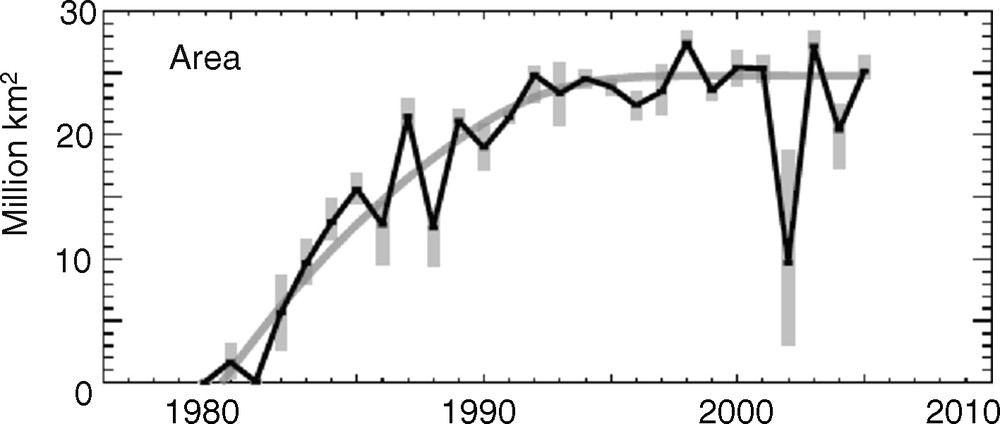
Area of the ozone hole for 1979–2005, averaged from daily total ozone area values contained by the 220-DU contour for 21–30 September. The grey bars indicate the range of values over the same time period. The grey line shows the fit to these values using Effective Equivalent Stratospheric Chlorine (EESC), an integral over all ozone depleting substances in the stratosphere (WMO, 2007).
Évolution de la surface moyenne du trou d’ozone entre 1979 et 2005, évaluée à partir de la région pour laquelle le contenu intégré d’ozone est inférieur à 220 DU, pendant la période du 21 au 30 septembre. Les traits gris indiquent la variabilité des valeurs pendant la même période. La ligne grisée montre l’ajustement à ces valeurs du contenu équivalent effectif en chlore (EESC) qui représente la somme de toutes les substances destructrices d’ozone, pondérée par leur efficacité individuelle de destruction de l’ozone (WMO, 2007).
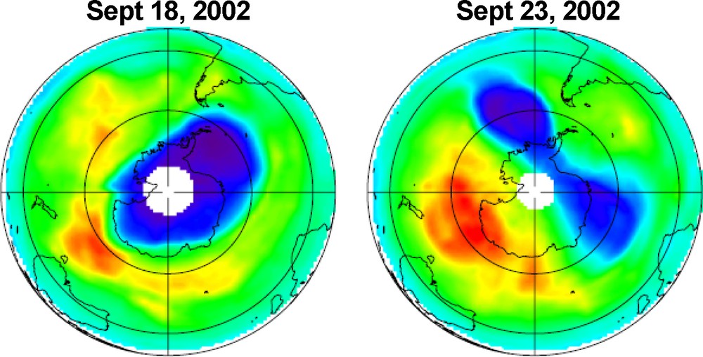
TOMS total ozone maps prior and during the major warming in September 2002. The white space around the South Pole is polar night where no measurements are made (WMO, 2007).
Cartes d’ozone total obtenues à partir des mesures TOMS avant et pendant l’échauffement majeur de septembre 2002. La région blanche autour du Pôle Sud représente la nuit polaire, pour laquelle aucune mesure TOMS ne peut être obtenue (WMO, 2007).
In the Arctic, the winter stratosphere is much warmer than in the Antarctic, due to stronger dynamical activity in the northern hemisphere. Arctic ozone loss during spring is highly variable depending on dynamical conditions, but it is anyhow much less severe than in the southern hemisphere. Maximum ozone loss in terms of integrated columns has not exceeded 30% since the early 1980s. For current halogen levels, anthropogenic chemical loss and variability in ozone transport are about equally important for year-to-year Arctic ozone variability. It is thus difficult to disentangle chemical and dynamical processes affecting ozone. A rather successful method is to use both Chemistry Transport Models (CTM) and satellite observations to infer chemical ozone loss (Deniel et al., 1998; Singleton et al., 2007). CTMs are atmospheric models that use meteorological analyses for the simulation of transport processes. This method, using CTMs passive ozone (not affected by chemical processes) and ozone fields from satellite observations, is illustrated in Fig. 7. It shows ozone loss in a very cold winter (2004/2005), computed from the SLIMCAT CTM (Chipperfield, 1999) and various satellite observations. All satellite instruments provided similar results, with a maximum inferred loss of 2–2.3 ppmv near 450 K (16 km). In addition to estimating ozone depletion, this technique is very useful for testing the understanding of chemical processes taking place in the Polar Regions through the comparison with the ozone loss simulated by the model.
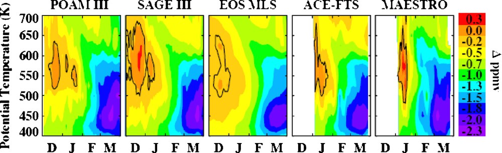
Daily cumulative chemical ozone loss (ppmv) inside the vortex during the 2004/2005 Arctic winter as a function of potential temperature inferred by differencing passive ozone calculated by the updated SLIMCAT chemical transport model, and ozone measured by the POAM III, SAGE III, Aura MLS, ACE-FTS, and MAESTRO instruments. Potential temperature is a surrogate for altitude in the stratosphere. The altitude range shown is about 14–26 km (Singleton et al., 2007).
Perte cumulée d’ozone (ppmv) à l’intérieur du vortex pendant l’hiver arctique 2004/2005, en fonction de la température potentielle. La perte d’ozone est calculée à partir de la différence entre un traceur passif d’ozone non affecté par les processus chimiques, simulé par le modèle de chimie-transport SLIMCAT, et les mesures satellitaires d’ozone obtenues à partir des instruments POAM III, SAGE III, Aura MLS, ACE-FTS et MAESTRO. La température potentielle est une fonction monotone de l’altitude dans la stratosphère. Le domaine spatial représenté est d’environ 14-26 km (Singleton et al., 2007).
7 Assimilation of satellite observations
Data assimilation is another important application for satellite observations of ozone and other stratospheric chemical species. Data assimilation is the combination of information from observations and models of a particular physical system in order to get the best possible estimate of the state of that system. Data assimilation methods were largely developed for operational weather forecasting, but in recent years, they have been applied to an increasing range of Earth Science disciplines and, more specifically, in Atmospheric Chemistry. There are many reasons for the assimilation of ozone observations:
- • data assimilation provides an improved mapping of ozone fields from multiple data sources;
- • it enables short-term ozone forecasts for the determination of surface UV radiation;
- • it is one of the best approaches for the estimation of tropospheric ozone at global scale, from the combination of satellite observation of stratospheric ozone with meteorological information provided by the model;
- • ozone data assimilation provides improved wind analyses as ozone measurements in the lower stratosphere contain information about the wind field, owing to the long photochemical lifetime of ozone in that region.
The assimilation of satellite ozone data has thus been the focus of several research groups in the last decades, with studies showing constant improvement in the state of the art. They have demonstrated the importance of having both total column observations as well as high-resolution profile information (e.g. Rood et al., 1989; Swinbank and Lahoz, 2003). As an example, the European Centre for Medium-Range Weather Forecasts (ECMWF) 40-year Reanalysis (ERA-40) is based on the use of a single, variational data assimilation scheme, which has processed observations from September 1957 to August 2002 in a consistent manner. For atmospheric ozone and water vapor, ERA-40 represents one of the largest continuous data sets available (Oikonomou and O’Neill, 2006). A new “ERA-Interim” dataset is in progress, with improved scheme for data assimilation and extended temporal coverage (Simmons et al., 2007).
8 The future of the ozone layer: evaluation of Chemistry Climate Models by satellite observations
With the expected decline of ozone depleting substances (ODS) linked to the Montreal Protocol, the next step is to predict the timing of the full recovery of the ozone layer. Owing to their generally long lifetime, the removal of ODS from the atmosphere will take several decades even with continued compliance with the Montreal Protocol. Ozone is expected to respond to these changes in ODS, but the timing and sensitivity of the response will depend on other factors, such as the increase in greenhouse gases, in particular CO2, that induce a cooling in the stratosphere, increase of the stratospheric water vapor content or increased emission of source gases such as N2O. Chemistry Climate Models (CCM) are important tools for predicting the future evolution of the stratosphere and the ozone layer, taking into account these changing conditions. These models include a full representation of dynamical, radiative and chemical processes in the atmosphere and their interactions. The feedback between chemical and dynamical processes is a major difference between CCMs and CTMs and such interdependencies are required to simulate the future evolution of ozone in a changing climate (Austin et al., 2003; Dameris et al., 2005).
While these models have substantially improved their climate simulations, there are still flaws in many models, including cold biases in the Southern Hemisphere and a lack of realistic tropical zonal wind oscillations. In that respect, satellite observations are important resources for model evaluation. A key question is how the current understanding of the stratospheric climate system fits together with temperature and constituent observations. This question is addressed by comparing past observations of ozone and other trace gases with various model simulations. In order to achieve a better understanding of model biases, quantities that are important for the simulation of ozone fields, like transport diagnostics, e.g. the mean age of air and the propagation of the annual cycle in water vapor, are validated against observations. The mean age of air can be inferred from observations of conserved tracers, as for example CO2, SF6 or HCl and HF. The age of air varies from 1 year in the equatorial lower stratosphere to 6 years in the high stratosphere. The annual variations in water vapor mixing ratios propagate vertically into the tropical stratosphere. This phenomenon, called “water vapor tape recorder”, is used to test the capacity of the models to simulate vertical transport in the Tropics. The comparison with water vapor observations from HALOE in a recent assessment of various CCMs simulations has shown a large spread in the results, indicating large differences in the representation of transport processes in the models (Eyring et al., 2006).
9 Conclusion and perspectives
Spatial observations have been a major contributor to the assessment of the ozone layer and the understanding of ozone balance as a function of latitude and height since the early 1980s. They have provided a comprehensive picture of the variability of ozone and atmospheric compounds that play a key role in stratospheric chemistry. The various satellite instruments developed in the last decades for the observation of the ozone layer have paved the way for the development of new sensors dedicated to other scientific issues such as air quality and climate change.
According to the latest estimates (e.g. WMO, 2007), recovery of the ozone layer is expected to occur around the middle of the 21st century as a result of the decrease of ozone depleting substances. Due to influence of future increases in greenhouse gas concentrations on the ozone layer and the reverse effect of future ozone changes on climate, particularly in the Southern Hemisphere, it is of utmost importance to continue the observation of the ozone layer with dedicated satellite instruments. Scientists recently raised concerns about the potential lack of global satellite ozone observation at the medium term (see the Athens statement at the 20th anniversary of the Montreal Protocol6). Indeed, the list of planned satellite observing systems shows that the capability for measuring ozone profiles will end at about 2015. These profiles characterize ozone in the lower and upper stratosphere, where the chemical loss is largest. The lack of such measurements might hinder the ability of the scientific community to assess the success of the Montreal Protocol with respect to the recovery of the ozone layer.
1 The Dobson Unit (DU) corresponds to the thickness of an atmospheric layer of pure ozone compressed to standard temperature and pressure (STP, 1 atmosphere surface pressure and 0 °C). Over the Earth's surface, the average thickness of the ozone layer is about 3 mm or 300 Dobson Units.
2 Scattering of the light by air molecules.
3 The quasi-biennial oscillation is an oscillation of the equatorial zonal wind between easterlies and westerlies in the tropical stratosphere, with a mean period of 28 to 29 months. The QBO has an effect on dynamical processes affecting ozone. Top: Deseasonalized, area-weighted seasonal (3-month average) total ozone deviations, estimated from different ground-based, satellite and merged datasets. Results are shown for the region 60°S–60°N (left) and the entire globe (90°S–90°N) (right). Bottom: The same plot, but for annual averages. (WMO, 2007). Panneaux du haut : évolution temporelle des valeurs mensuelles d’ozone total désaisonnalisées, pondérées par la surface et moyennées sur trois mois, calculées à partir de différentes mesures sol, satellitaires ou de données fusionnées. Résultats pour la bande de latitude 60 °S–60 °N (panneau de gauche) et pour le globe (90 °S–90 °N, panneau de droite). Panneaux du bas : mêmes résultats, mais pour des moyennes annuelles (WMO, 2007).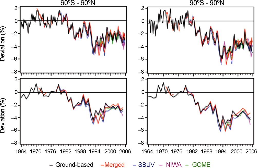
4 http://www.wmo.int/pages/prog/arep/gaw/ozone/.
5 http://ozonewatch.gsfc.nasa.gov/.
6 Athens statement: http://ioc.atmos.uiuc.edu/press/ATHENSSTATEMENT2007.pdf.