

1 Introduction
The Aveiro region, on the Northwest Portuguese coast, is densely populated. Industry and agriculture are intense and pressure on the Earth's resources and land development grows constantly. Geomorphologically, the Aveiro basin is a coastal region characterized by gentle topography and lowlands. Thus it has a high degree of vulnerability to sea level changes. In fact, the Atlantic Ocean stress on the coastal regions of the Aveiro Basin has been increasing steadily. It causes evident side effects on land development and management as well as on groundwater resources and exploitation. Stress is expected to increase as climate change effects accumulate.
Understanding the structure of the Aveiro basin is therefore very important. Detailed knowledge of the structure of the basin can provide useful information and guidance for the exploration and exploitation of groundwater resources, strategic decisions on land development and for the investigation of offshore structures and potentialities.
Bearing in mind the geological, geographical and geomorphologic conditions of the basin, the gravity method is well suited to provide geological and tectonic information of the region. A first pioneer work (Casas et al., 1995) demonstrated the suitability of the application of gravity methods to the study of the Aveiro basin as a fast, reliable and economic method to survey the area.
A detailed geophysical survey of the Aveiro basin was carried out later. Hence, information based on deep electrical soundings, existing boreholes and a gravity map covering the whole area was compiled (Figueiredo, 2001). In that work all the available geophysical data were integrated, but only limited two dimensional gravity data modelling was used. Nevertheless this modelling was constrained by all the information gathered and constituted the basis for further and more detailed work.
The gravity survey consisted of 653 readings covering the area with an average density of four readings per km2. A regional and residual map for the area and a two dimensional (2D) gravity model were produced using data from this survey and the results of its preliminary modelling are the starting point to further process and reinterpret the Aveiro basin gravity data as presented in this article.
Thus the aim of this work is to obtain a more detailed model for the Aveiro basin. Thus gravity data were used to compute the gradient, the second vertical derivatives and the continuation of the original gravity field. This procedure will be followed by detailed 2D modelling, using north–south as well as east-west profiles, so that a more comprehensive tectonic map of the region is produced. This map will be interpreted on the basis of the findings of the gradients, derivatives and continuations maps.
The inherent difficulties and ambiguities of the interpretation of potential field data will be reduced by the integrated use of all these analytical techniques in conjunction with all the available geological and borehole data. Finally, the gravity-based model proposed for the basin will be compared with the previous tectonic model and the benefits of the proposed interpretation will be addressed.
1.1 General Geology of the Area
Earlier geological maps for the Aveiro district were produced by Barbosa, 1981; Teixeira and Zbyszewski, 1976. More recently the geology of the area was discussed and reviewed in Silva, 1990. This work included the information from the boreholes drilled in the basin. These boreholes were drilled for water exploration and exploitation purposes and allowed an overall view of the basin structure. However, these boreholes do not cover the basin evenly and some of them do not reach the crystalline bedrock. It is impossible to draw a more detailed image of the Aveiro basin from the borehole information, but nevertheless, they provide the most useful information for the interpretation of any geophysical data in the region.
A general simple sketch of the surface geology of the area is shown in Fig. 1 (after Casas et al., 1995). In broad terms, the Aveiro basin, locally called “Ria de Aveiro”, is the most northerly part of the Portuguese Western Mesozoic Margin also called the “Lusitana Basin”, Silva and Andrade, 1998. It is a sedimentary basin, adjacent to the Hesperian massif, craton border type and with low subsidence where sedimentation occurred over the continental crust. The Precambrian basement is located at absolute heights ranging from −200 to −500 m in the coastal zone. Outcrops in the eastern part of the basin, near the Hesperian craton, show that the basin is affected by strike slip faulting (Mougenod et al., 1986). The succession of deposits over the Precambrian basement includes Triassic sandstones and Medium to High Cretaceous deposits, covered in places by old beaches and fluvial Pleistocene deposits. In the coastal zone, these deposits are covered by Recent Holocene sediments (Fig. 1).
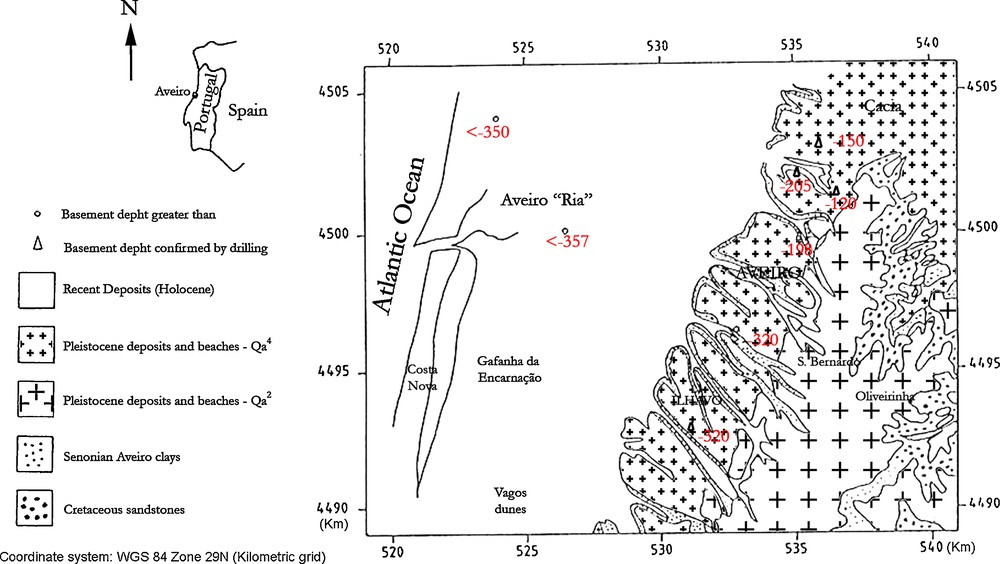
General Surface Geology of the Aveiro basin (after Casas et al., 1995). The numbers represent the depths of the crystalline basement in metres.
Géologie de surface du bassin d’Aveiro (d’après Casas et al., 1995). Les nombres représentent les profondeurs du soubassement cristallin en mètres.
The region belongs to the so-called Western Mesocenozoic Margin, Lusitanian basin. Two major fracture systems have been recorded, striking north–south and NNW–SSE. In accordance with Silva and Andrade (1998), these systems represent the reactivation of Variscan strike-slip faults well known in the basement outcropping east of Aveiro. A further NNW–SSE system has also been recorded and could be related to the Late Hercynian deformations (Silva and Andrade, 1998).
The sedimentary formations of the Lusitana basin show little deformation. However, post Hercynian movements caused fractures in the basement and horsts and grabens were produced. As a result, various blocks of individual shape and development were created (Barbosa, 1981; Casas et al., 1995; Teixeira and Zbyszewski, 1976).
The first model of the topography of the basement was proposed by Ribeiro et al., 1972. Based on data from boreholes a more elaborate model was constructed by Silva and Andrade (1998) and is depicted in Fig. 2. It is clear from the analysis of Fig. 2 that there is more information in the northern part of the basin. The interpretation of the southern part of the basin is less accurate. The basement generally plunges to the southwest reaching depths greater than 400 m in its deepest part. It is not possible to interpret graben-like structures over the entire basin from Fig. 2. This behaviour is particularly evident in the Northeast part of the region, where more borehole information is available. The preliminary gravity works (Casas et al., 1995; Figueiredo, 2001) provided similar information to this model and confirmed the graben-like structure over the entire Aveiro basin.
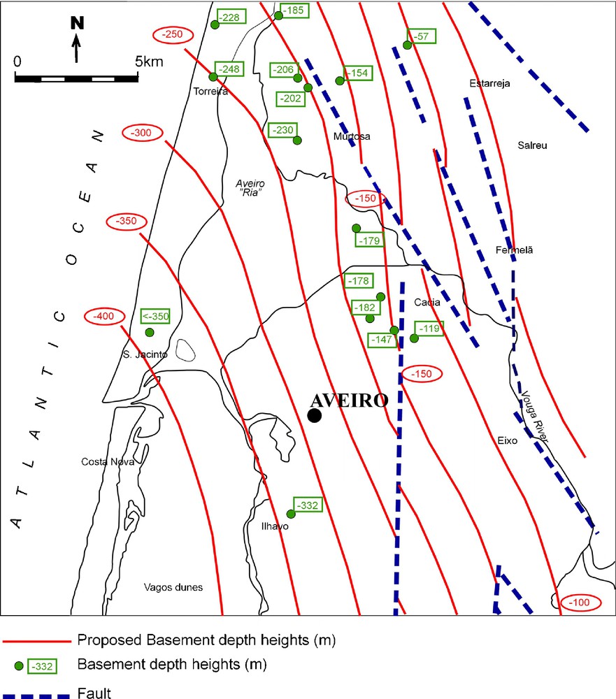
Tectonic model and basement depths after Silva and Andrade (1998). The proposed main fractures are shown in dashed lines, the depths in metres of the bedrock measured in boreholes are given in boxes and, finally, the solid curves represent the basement depths as interpreted by the authors. The two main orientations of the fractures, north–south and NNE–SSW, were interpreted and plotted using dashed lines.
Modèle tectonique et profondeurs du soubassement, d’après Silva et Andrade (1998). Les principales fractures proposées apparaissent en lignes tiretées, les profondeurs en mètres du soubassement mesurées dans les forages sont encadrées et les courbes représentent les profondeurs du socle telles qu’elles sont interprétées par les auteurs. Les deux orientations principales des fractures, nord-sud et NNE–SSW ont été interprétées et représentées en utilisant des lignes tiretées.
Thus the present study is also intended to contribute to a better understanding of this region. In fact, the gravity survey took place over an area where recent Quaternary formations cover older sedimentary rocks. It is therefore not possible to map the location of fractures and deformations correctly. It is expected, from density estimates on borehole rock samples (Figueiredo, 2001) that the major density contrast will be between the sedimentary cover and the basement. Thus, in the present work mainly the depth of the basement will be investigated and modelled.
2 Gravity data processing
As mentioned previously, regional gravity data over the Aveiro basin region from an earlier survey (Figueiredo, 2001) were considered. The gravity survey was carried out with a Lacoste and Romberg model G gravimeter, over a random grid with distances between measuring points of less than 500 m. A total of 653 stations were measured and coordinates were taken from topography surveys available from local councils and hipsobathimetric surveys. The coordinates used the UTM, Fuse 29, International Ellipsoid European Datum, scales 1:10,000 and 1:25,000. Density estimates and calculations were taken from borehole samples as well as the Parasnis method together with Nettleton profiles/Jung correlation coefficient, Parasnis, 1997.
The first stage of the processing was the determination of the regional gravity field. Two methods were applied to separate the regional and local gravity field:
- (i) a plane regional field model;
- (ii) a third-order surface regional field model.
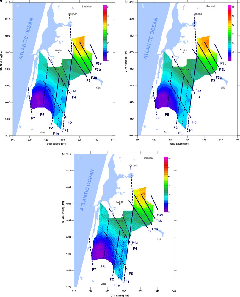
Fig. 3 shows the Bouguer anomaly map of the basin, the input data for this work, (Fig. 3a), the residual gravity map obtained with a first order plane as a regional field model (Fig. 3b) and on the Fig. 3c the residual gravity map calculated from a regional field modelled as a third order surface.
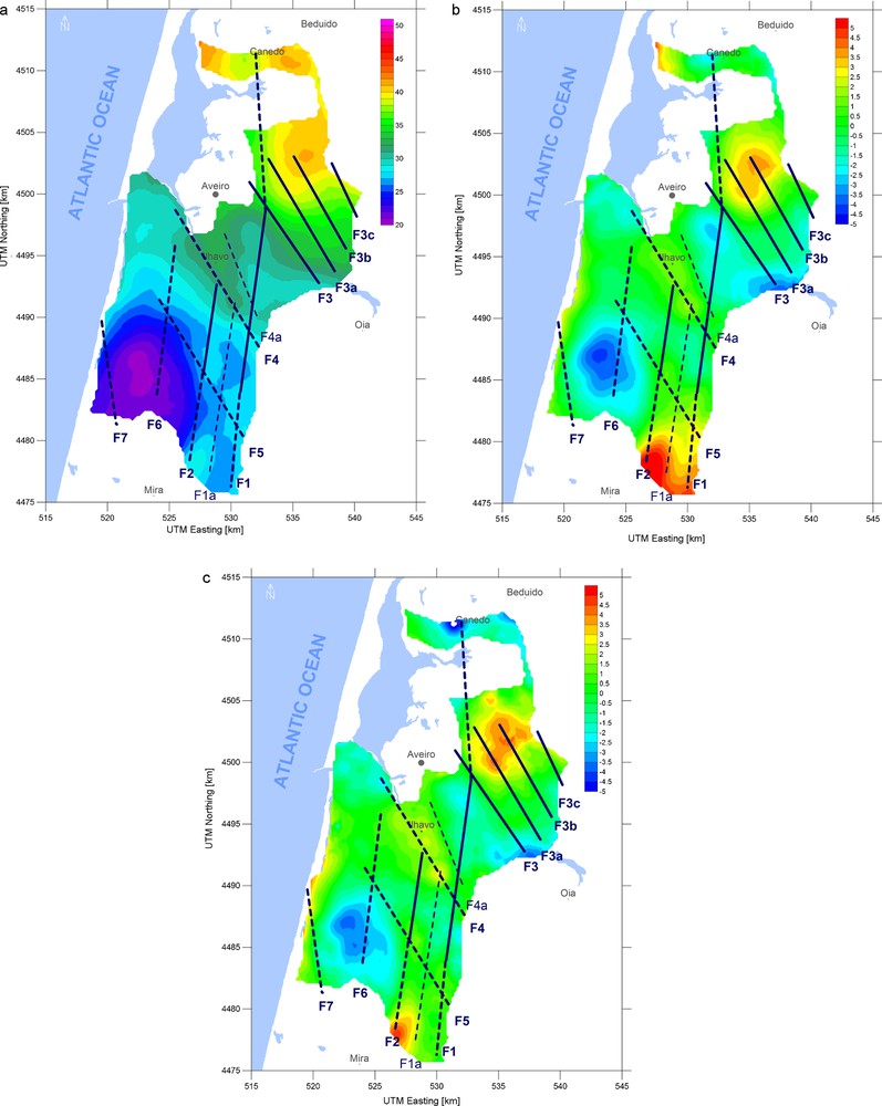
(a) Bouguer anomaly map; (b) residual field after the removal of linear trend; (c) residual field after the removal of the regional field modelled by the 3rd order surface. Gravity values are expressed in mGals (1 mGal = 10−5 m.s−2). Interpreted known tectonic features are plotted in solid blue lines while newly proposed structures are plotted in dashed blue lines.
(a) Carte de l’anomalie de Bouguer ; (b) champ résiduel après élimination de la tendance linéaire ; (c) champ résiduel après élimination du champ régional modélisé par la surface de 3e ordre. Les valeurs de gravité sont exprimées en mGals (1 mGal = 10−5 m.s−2). Les caractéristiques tectoniques connues sont représentées par des lignes bleues continues, tandis que les structures nouvellement proposées le sont par des lignes tiretées bleues.
Therefore, in Fig. 3b the influence of local structures is clearly shown after removing the regional gravity field – gr – modelled as the straight plane fitted with the first order polynomial regression. On the other hand, Fig. 3c shows the local field after removing the regional field modelled as the third order surface. Over these maps the tectonic features depicted in Fig. 2 were drawn as solid blue lines while the dashed blue lines represent the new proposed structures as described later.
In general, the Bouguer anomaly map in Fig. 3a shows the overall shape of the basin with the most pronounced structures. The analysis of the map shows that to the northeast higher values are revealed and the basement must therefore be closer to the surface in this area. The lowest values are depicted to the southwest and are a result of the deeper basement in this region. This is in broad agreement with the map in Fig. 2. However there are two new and distinct NW–SE alignments at the centre of the map, depicted as blue dashed lines F4 and F5.
The maps in Fig. 3a and Fig. 3b, corresponding to the residual field, give a clearer picture of local structures and their characteristics. In particular, the local field after the third order surface removal, Fig. 3c, emphasizes the local structural details while the overall basin shape and the most pronounced anomalies disappear. Thus, the analysis of the gravity field after regional model removal is suitable for the determination of local tectonic features at the bottom of the basin while the overall basin shape is suppressed.
3 Horizontal gradients and second vertical derivatives maps
In the next step of the processing, the horizontal gradients of the anomalous field were computed. Horizontal gradient in the x (east–west) and y (north–south) direction, is defined as the estimation of the corresponding directional derivative of the gravity field in the particular direction. After Blakely, 1995, p. 324, if the gravity field is uniformly sampled in x direction, the directional derivative at the location with coordinates xi,yj can be estimated by the formula
| (1) |
The estimation ΔGx(xi, yi) is the value of the horizontal gradient in the x direction for the location xi,yj. Similarly, the horizontal derivative in the y direction can be estimated with the appropriate horizontal gradient ΔGy(xi, yi):
| (2) |
Because of their definition, the horizontal gradients of the gravity field should reach extreme values at the edges of structural blocks where change in density or depth of structures occurs. Nevertheless, this effect is strongly direction-dependent. The east–west horizontal gradient field reaches its maxima and minima on the north–south oriented structures and the east–west structures are suppressed and vice-versa.
In order to obtain directionally independent indicator of lateral changes in density distribution, vertical derivatives of the gravity field were used. The second vertical derivative of the potential field φ on the horizontal surface is the direct consequence of the Laplace's equation for the potential field (after Blakely, 1995, p. 325):
| (3) |
While it is, in general, impossible to solve this equation in the real domain, it can be converted to the Fourier domain:
| (4) |
Hence, the second vertical derivative of the gravity field can be computed using the Fourier domain operations as a three-step filtering operation. First, the gravity field is transformed to the Fourier domain. Then the transformation result is multiplied by |k|2. Finally, the product is transformed back to the real domain. Numerical methods such as the multi-dimensional discrete Fourier transform (Press et al., 1986) can be applied to compute the estimation of the second vertical derivative of the evenly spaced matrix of discrete gravity values.
However, the application of vertical derivatives to the real field data has a significant limitation as the computation of the vertical derivatives behaves as a high-pass filter. The influence of structures with high wave numbers, i.e. short wavelengths, is amplified while the influence of large structures is suppressed. The side effect of this procedure is significant amplification of noise included in the gravity signal. Random noise is high-frequency by its nature and its amplification can superpose any useful information significantly.
As mentioned above, it is not possible to find the general analytical solution of the Eq. (3) in the real domain. Several authors derived formulas for numerical calculation of the estimation of second vertical derivative from discrete matrix data based on simplified theoretical models, e.g. the Elkin's formula (Elkins, 1951). Elkin's formula can be used for estimating the second vertical derivative in a node of rectangular grid as a linear combination of the value of the gravity field in the node under study and values in the 16 surrounding nodes.
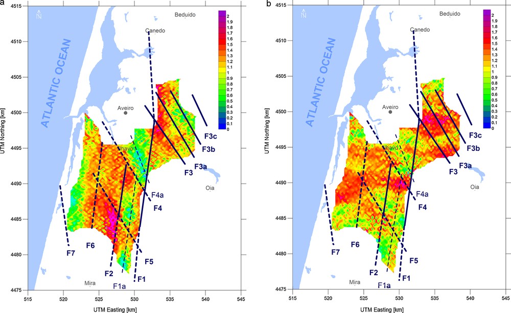
As shown in Fig. 2 the expected fractures have two main directions, that is, north–south and NNW–SSE. So, in order to extract as much information as possible from the gravity gradients maps, these were computed in the north–south and in the east–west directions separately. The Gravity Horizontal Gradients for the Aveiro Basin are depicted in Fig. 4. Hence Fig. 4a shows the horizontal gravity gradients computed in the east–west direction. In this case, tectonic structures running approximately from north to south should be visible as maxima and minima on this map. On the other hand Fig. 4b shows the north–south horizontal gravity gradient. In this case it is expected that east–west tectonic features are emphasized. Care should be taken when interpreting the map on the Fig. 4b because the east–west direction is not expected to be a dominant tectonic direction.
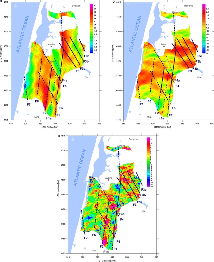
Gravity horizontal gradients and second vertical derivative field together with the possible linear tectonic features interpreted from these fields plotted as blue lines. (a) east–west horizontal gradient in mGal.km−1; (b) north–south horizontal gradient in mGalkm−1 and (c) second vertical derivative of the gravity field computed by Elkin's method in mGal.km−2.
Gradients horizontaux de gravité et champ de dérivée verticale seconde avec les traits tectoniques linéaires interprétés à partir de ces champs représentés par des lignes bleues (a) gradient horizontal est–ouest en mGal.km−1 ; (b) gradient horizontal nord–sud en mGal.km−1 et (c) dérivée verticale seconde du champ de gravité, calculée par la méthode d’Elkin en mGal.km−2.
Three methods for the computation of second vertical derivatives of the gravity field were also tested in the Aveiro region, that is, the Elkin's method, the Rosenbach's method, and finally the approach based on transformation of the gravity field in Fourier domain described above. These three methods produced similar results and there were no significant differences in the interpretation of their data in the Aveiro basin. However, the second vertical derivative field calculated by the Elkin's method is less noisy than the others, Fig. 4c.
As mentioned earlier, the advantage of the second vertical derivative field is its independency on the direction of structures. Alignments of maxima or minima at the second derivatives map should follow the positions of linear geological structures. As can be seen from the Fig. 4c, due to the noise amplification effect of the transformation, the resulting field is not as clear as the horizontal gradients.
Possible linear tectonic features were interpreted from the horizontal gradient and vertical derivative maps. These lineaments are plotted as dashed blue lines in the maps of Fig. 4. The dominating north–south features are clearly visible on the map at Fig. 4a. On the other hand, the NNW–SSE features are not so clear and the compilation of information from all three maps is required to locate them.
The most important features dominating the Fig. 4a and 4c are two north–south oriented structures interpreted as the faults F1 and F2 in Fig. 4. Northernmost part of them can be identified at the south-eastern edge of the map in Fig. 2 as a couple of parallel north–south faults. Parallel to the faults F1 and F2 in Fig. 4 closer to the Atlantic coast runs the fault F6. It delineates the eastern edge of the deepest part of the Aveiro basin.
The second important direction of faulting of the Aveiro basin is NNW–SSE. The graben-like structure heading in this direction is delineated by the faults F3 and F4a in the maps in Fig. 4. The fault F3 has its equivalent in Fig. 2, while the fault F4a is the result of the gravity field interpretation. Parallel faults F3a, F3b and F3c have their equivalents in Fig. 2. Location of the individual faults of this fault system is approximate because the gravity signal is noisy in this part of the region under study. Finally, the fault F5 runs more or less parallel to the fault F4 5 km to the southwest. This fault is not located in the region covered by Fig. 2.
4 Downward continuation maps
The downward continuation of the Bouguer gravity field was computed as the final step of the gravity field analysis. Downward continuation is a mathematical transformation of the values of a potential field measured on a given flat surface to the values that would be measured at the surface located closer to the sources.
It can be shown, that if there is the known distribution of the potential field U over the infinite level surface z0, it is possible to compute the value of U at another level surface z0 + Δz, for details see e.g. Blakely, 1995, pp. 313–316:
| (5) |
The equation (5) is the downward-continuation integral. It is not necessary to know anything about the distribution of the sources. The only assumption is that all the sources of the field U are below the surface z0.
It is computationally extensive to compute the 2D integral for each point of the new surface z0. Fortunately, Eq. (5) can be transformed to the Fourier domain:
| (6) |
Practical computation of the level-to-level downward continuation can be provided similarly to the computation of the vertical derivatives.
In the case of the transformation of Bouguer gravity anomalies, these anomalies are caused by blocks of rocks with densities differing from the density used for calculating the Bouguer anomalies. If all the anomalous objects are deep below the surface, their gravity signal is weak. After the downward continuation of the surface field is computed, the signal originated from the anomalous object under study is amplified in the transformed field. The downward continuation transformation can only work correctly as long as the transformed surface does not reach the depth of any source object, i.e. all source masses are below the transformed surface. When the depth of the mass sources, e.g. the bottom of the basin, is reached, the computed gravity field is totally distorted because continuing into sources is not allowed.
As can be seen from Eq. (6), downward continuation of the gravity field behaves as a strong high-pass filter. Amplitudes of short-wavelength signals are significantly amplified and problems can arise because of strong noise and aliasing effects amplification.
Level to level downward continuation in Fourier domain was applied to the Bouguer anomaly field of the Aveiro basin for three different depths of continuation Δz, 100 m, 200 m and 300 m. The maps of the downward continued gravity field of Aveiro basin are plotted in Fig. 5, together with the lineaments interpreted from the gradient data.
Downward continued gravity field of Aveiro basin in mGals for three different depths of the transformation surface, (a) 100 m, (b) 200 m, (c) 300 m.
Champ de gravité continu descendant du bassin d’Aveiro en mGals pour 3 profondeurs différentes de la surface de transformation, (a) 100 m, (b) 200 m, (c) 300 m.
Comparing the three downward continued maps of the Bouguer field illustrates the behaviour of this transformation. With increasing depth of transformation more detailed structure of the basin bottom should appear. This feature can be noticed e.g. by the comparison between Fig. 5a and 5b and the original Bouguer map from the Fig. 3a. The gravity field in the southern part of the rectangular region delimited by the lineaments F1, F2, F4 and F5 is shaped as one small negative and one small positive anomaly. While in Fig. 3a these anomalies are very weak and unclear, the negative (dark blue) anomaly is more pronounced in Fig. 5a and the positive (light blue) anomaly is clearly noticeable in the Fig. 5b as the level of observation comes closer to the basin bottom.
Similar behaviour can be observed e.g. for the detailed shape of the centre of the largest negative anomaly to the west of the southern end of the lineament F6. While on the original Bouguer map the anomaly has the shape of a simple oval, with increasing depth of observation two minima are separated on the northwest and southeast edge of the anomaly – compare Fig. 5a, 5b and 5c.
The comparison of the maps in Fig. 5a to 5c with increasing depths of the continuation also illustrates the unpleasant effect of noise amplification caused by the downward continuation procedure described above. In Fig. 5c the whole map is affected by the noise caused by gridding of the input gravity field called aliasing effect. Grid size of 250 m was used for gravity data sampling. Harmonic aliasing derived from the 250 m wavelength creates rectangular shape noise over the gravity signal. This type of noise is visible on some parts of the map in Fig. 5b and is a dominating feature in Fig. 5c. Structural details, which should be depicted by the downward continuation are overlapped by the strong noise. This effect is clearly visible e.g. on the two small anomalies at the southern part of the area delimited by the lineaments F1, F2, F4 and F5 described above. Both of these anomalies are overlapped by the noise on the Fig. 5c.
The increasing level of noise is the limiting factor for the further processing of the downward continued gravity field in the Aveiro Basin area. The deepest possible continuation where a reasonable signal-to-noise ratio can be achieved is 200 m. The 200 m downward continued Bouguer field was chosen for the computation of horizontal gradients. Fig. 6 shows the horizontal east–west and north–south gradients computed from the 200 m downward continued gravity field of the Aveiro basin. Comparison of Fig. 6 with Fig. 4a and b demonstrates the effect of downward continuation. Amplitudes of all horizontal gradient anomalies are magnified due to the observation point being moved closer to the mass bodies. This feature is most pronounced on the intersections of interpreted structures, e.g. F1 and F3 in both directions. Several secondary linear features become pronounced at the Fig. 6a and 6b, structure F1a running in the centre between structures F1 and F2 and structure F4a running approx. 2 km to the ENE from the structure F4. All these phenomena were taken into account in the gravity modelling.
Horizontal gradients computed from the 200 m downward continued gravity field of the Aveiro basin: (a) east–west direction; (b) north–south direction.
Gradients horizontaux calculés à partir du champ de gravité continu descendant à 200 m, du bassin d’Aveiro: (a) direction est–ouest; (b) direction nord–sud.
5 Gravity modelling
Based on the data processing described in the previous chapter, two detailed gravity models were constructed:
- • the first model is based on the Bouguer anomaly field (Fig. 3a) modelling the overall shape of the basin and the major structures. The depth of the sedimentary coverage of the basin was constrained by available geological and geophysical data, i.e. drill logs and geological profiles interpreted from deep resistivity sounding data (Figueiredo, 2001);
- • the other model is based on the residual gravity field as plotted in Fig. 3c. The overall shape of the basin is suppressed in this model, but more pronounced details of the buried tectonic structures are visible.
According to the geological setting of the Aveiro basin, four geophysical layers were defined for gravity modelling. The definition of the geophysical layers can be found in Table 1. Rock densities used for modelling of the corresponding geophysical units were estimated from the rock samples from boreholes.
Propriétés des couches géophysiques utilisées pour la modélisation de gravité.
| Geological unit | Rock density [g.cm−3] | Cross-section block colour (Figs. 7 and 8) |
| Quarternary sediments | 2.20 | Yellow |
| Cretacious deposits | 2.40 | Dark green |
| Triassic sandstones | 2.55 | Light green |
| Precambrian basement rock | 2.65 | Orange |
The GM-SYS 2¾-D Gravity Modelling Software (http://www.nga.com) was used for gravity modelling. Each model consists of two sets of perpendicular 2500 m distant profiles. Thus, seven north–south profiles emphasize the east–west structures, while thirteen east–west profiles show mainly the north–south tectonic structures over the Aveiro basin. The characteristics of the particular gravity models are summarized in Table 2.
Caractéristiques des modèles de gravité individuels sur des profils nord–sud et est–ouest.
| Profile name | Coordinates | Bouguer field model | Residual field model | ||||
| UTM Easting [km] | UTM Northing [km] | Length [km] | Observed gravity range [mGal] | Model RMS error [mGal] | Observed gravity range [mGal] | Model RMS error [mGal] | |
| NS1 | 522.5 | 4482.0–4501.5 | 19.5 | 20.7–30.6 | 0.100 | −3.7–1.0 | 0.092 |
| NS2 | 525.0 | 4481.5–4500.0 | 18.5 | 21.9–30.5 | 0.138 | −2.7–0.6 | 0.067 |
| NS3 | 527.5 | 4477.0–4512.0 | 35.0 | 25.3–42.1 | 0.113 | −0.7–3.8 | 0.296 |
| NS4 | 530.0 | 4475.5–4511.0 | 35.5 | 26.3–39.5 | 0.101 | −2.2–2.6 | 0.122 |
| NS5 | 532.5 | 4488.0–4511.5 | 23.5 | 29.1–39.5 | 0.294 | −2.7–2.2 | 0.117 |
| NS6 | 535.0 | 4491.5–4512.0 | 20.5 | 29.5–41.3 | 0.146 | −2.7–4.0 | 0.134 |
| NS7 | 537.5 | 4492.5–4507.5 | 15.0 | 29.7–40.6 | 0.128 | −3.6–3.3 | 0.125 |
| EW1 | 527.5–536.5 | 4511.0 | 9.0 | 38.2–41.3 | 0.183 | −5.0–0.4 | 0.120 |
| EW2 | 531.0–538.0 | 4505.0 | 7.0 | 35.4–40.5 | 0.097 | −1.8–3.1 | 0.107 |
| EW3 | 532.0–537.5 | 4502.5 | 5.5 | 36.5–41.0 | 0.076 | 0.4–4.0 | 0.069 |
| EW4 | 521.5–540.5 | 4500.0 | 19.0 | 29.4–38.9 | 0.107 | −1.8–4.1 | 0.115 |
| EW5 | 521.5–540.0 | 4497.5 | 18.5 | 28.9–35.2 | 0.079 | −2.0–0.9 | 0.063 |
| EW6 | 521.5–540.0 | 4495.0 | 18.5 | 28.9–33.7 | 0.075 | −1.4–1.9 | 0.088 |
| EW7 | 521.0–538.5 | 4492.5 | 17.5 | 27.1–31.3 | 0.086 | −3.6–3.0 | 0.122 |
| EW8 | 520.0–533.0 | 4490.0 | 13.0 | 24.7–30.3 | 0.094 | −1.1–3.0 | 0.127 |
| EW9 | 519.5–532.0 | 4487.5 | 12.5 | 21.3–28.6 | 0.098 | −3.5–2.5 | 0.119 |
| EW10 | 519.0–532.0 | 4485.0 | 13.0 | 20.6–27.3 | 0.109 | −3.5–1.5 | 0.101 |
| EW11 | 519.0–532.0 | 4482.5 | 13.0 | 21.1–27.6 | 0.117 | −2.3–1.7 | 0.078 |
| EW12 | 526.0–531.0 | 4480.0 | 5.0 | 24.1–27.6 | 0.099 | −0.4–2.3 | 0.059 |
| EW13 | 527.0–531.0 | 4477.5 | 4.0 | 26.4–28.6 | 0.067 | −0.5–4.4 | 0.076 |
| Average | 0.117 | 0.109 |
Two examples of gravity modelling results are shown in Fig. 7 for both Bouguer field and residual field. Density distribution models based on gravity fields analysis for all profiles are plotted in Fig. 8.

Examples of gravity models. In the upper part of each plot the observed gravity field plotted by black circles and the response of the model plotted by thin black curves are shown. Differences between the observed and modelled gravity values are plotted in red. The lower part of each plot shows the vertical cross-section over the profile with the distribution of geophysical layers (Table 1) corresponding to the plotted gravity response.
Exemples de modèles de gravité. Dans la partie supérieure de chaque repère, le champ de gravité observé et représenté par des cercles noirs et la réponse du modèle représentée par de fines courbes noires sont montrés. Les différences entre les valeurs de champ observées et modélisées sont représentées en rouge. La partie inférieure de chaque repère montre la coupe verticale sur le profil avec la distribution des couches géophysiques (Tableau 1) correspondant à la réponse gravitaire figurée.
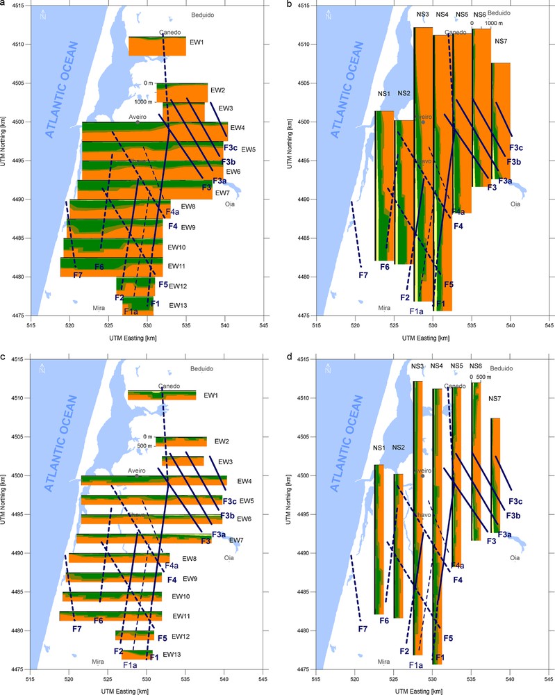
Density distribution models based on gravity field analysis: (a) Bouguer field model east–west profiles; (b) Bouguer field model north–south profiles; (c) Residual field model east–west profiles and (d) Residual field model north-south profiles.
Modèles de distribution de densité basés sur l’analyse de champ gravitaire : (a) Profils est–ouest de modèle de champ de Bouguer ; (b) Profils nord–sud de modèle de champ de Bouguer ; (c) Profils est–ouest de modèle de champ résiduel ; (d) Profils nord–sud de modèle de champ résiduel.
The map of the basin bottom shape was plotted as the final step of the modelling (Fig. 9). The map was constructed as the depth of the interface between the Triassic sandstone and the Precambrian basement rock geophysical layers as interpreted from the models at the Figs. 8a and b.
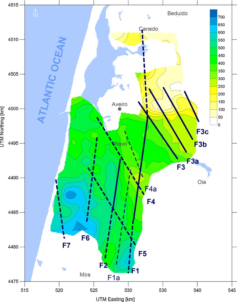
Map of the tectonic features interpreted from the gravity data analysis together with the basement depths for the Aveiro basin in meters interpreted from gravity model.
Carte des traits tectoniques interprétés à partir de l’analyse des données gravitaires, avec les profondeurs du socle pour le bassin d’Aveiro en mètres, interprétées à partir du modèle gravitaire.
6 Gravity data interpretation
Detailed analysis of the gravity field of Aveiro basin made it possible to construct a detailed mass distribution model. The gravity model consists of two parts, that is, interpretation of tectonic features and basin shape modelling (Fig. 9).
The interpretation of the tectonic features is based primarily on the gravity field analysis. Horizontal gradients and Elkin's second vertical derivatives were very useful at this stage of interpretation. Then the interpreted features were compared to the gravity models both using the Bouguer field and the residual field. Based on the results, the gravity models have been constrained and, as necessary, interpreted tectonic features were repositioned to fit the model properties.
To better demonstrate the process of the interpretation of the tectonic structures, the final result of the interpretation of the tectonic structures is drawn over each map in Figs. 3, 4, 5, 6 and 8.
Detailed comparison of the interpreted lineaments on the northern part of Fig. 9 and Fig. 2 shows similarities in the interpreted fault structures. Lineament F1 in Fig. 9 is similar to the dominating north–south fault positioned 2 km east of the town of Aveiro in Fig. 2. Similarly, the group of lineaments F3 to F3c in Fig. 9 could be paired with the group of parallel faults in the north–east part of the map in Fig. 2. The structure F4 in Fig. 9 can be interpreted as a possible continuation of the short fragment of the NNE–SSW fault. Its northernmost part is plotted at the south–east edge of the map in Fig. 2.
A new important structure is the fault F6 in Fig. 8. This linear structure is expected to run from the south to the north approximately up to the latitude of the town of Ilhavo and represents a deep structure buried below the basin sediments. The fault structure F6 delineates the eastern edge of the deepest part of the Aveiro basin, while the western edge is approximated by the linear structure F7.
Finally, a new map of the basin depth based on the gravity mass distribution model was constructed (Fig. 9). This map gives much more detailed estimates of the basin depths than the previously published (Figs. 1 and 2). While the bottom of the basin in general subsides from the northeast to the southwest, the subsidence does not seem to be as smooth as presented in other models (Silva and Andrade, 1998). The graben-like bottom structures are clearly visible from the gravity data interpretation in north–south and NNW–SSE directions, which leads to the conclusion that the basin bottom shape is more complex.
The comparison of the basement depths map in Fig. 2 to the gravity modelling results as presented in Fig. 9 shows that the overall increase of the basement depth in the NE–SW direction as well as overall basement depths are similar on both models. In addition, graben-shaped and rift-shaped structures are clearly distinguishable in both north–south and NNW–SSE directions.
The most pronounced north–south structures are represented by the deepest part of the Aveiro basin delineated by the structures F6 and F7 as well as the graben structure to the west of fault F2 and the rift-shaped structure delimited by the faults F1 and F2. The biggest graben structure of the NNW–SSE direction is delimited by the lineaments F3 and F4a and the rift structure of the same direction is delimited by the faults F4a and F4.
The increase of the depth of the basin bottom in the NE–SW direction is not smooth. The interpreted lineaments F3, F4 and F5 delineate areas of about 100 m steps, while the basin bottom is more or less flat between these steps.
7 Conclusions
The new interpretation of the gravity data of the 2001 regional gravity survey of the Aveiro results in a detailed model for the basin shape and tectonic structures buried below the Quaternary sediments.
A detailed map of the basin bottom depths and the proposed tectonic features are presented as interpreted from the gravity data (Fig. 9). In comparison with the previously published results (Fig. 2) the model presented in this study is much more detailed. It is evident from the analysis, that the structure of the basin bottom can be described as a superposition of graben-like and rift-like structures of different directions. It corresponds to the available data about the geology of the basin. The presented interpretation covers the whole extent of the Aveiro basin with the exception of the swamp area “Ria de Aveiro” where the setting up of gravity stations was impossible.
The results represent the unique quantitative geophysical mass distribution model as derived from the comprehensive interpretation of the data set of the basin. The data processing procedure was applied in the same manner over the whole area under investigation. Modelling parameters were constrained to the available geological, borehole and geophysical data. Thus, the presented model is well established and homogenous over the whole area including parts of the region without further reliable geological or geophysical information.
Detailed knowledge of the internal structure of the basin is of great importance for the future investigation and exploration of the whole region. The results presented represent useful tools for future underground water exploration and exploitation as well as borehole location planning. Bearing in mind the geomorphology of the basin the gravity method proves to be an economical tool for investigating basin structures.
Acknowledgment
The authors wish to acknowledge the support from the EU Erasmus program and the partial support from the Research Project no. 0021620855 of the Ministry of Education, Youth and Sports CR.
The authors are grateful to the reviewers for their valuable remarks.