

1 Introduction
At a global scale, the Earth has many discontinuities, such as the Mohorovicic discontinuity, as the discontinuities in the mantle at 220 km and 400 km (Dziewonski and Anderson, 1981). The Earth also has some lateral or vertical heterogeneities at different scales that are related to the change in the physical or chemical properties (e.g., phase changes, partial melting) in the lithosphere and mantle, and even in the inner core (Anderson, 2006; Ben-Zion and Lee, 2006; Vidale and Earle, 2000). Seismic waves will show different levels of artificial anisotropy when they propagate through these discontinuities and heterogeneities, which will depend on their spatial scales and the seismic wavelength. Indeed, much information on the structure of the Earth is ‘filtered’ away when seismic waves pass through these discontinuities and heterogeneities, especially at high frequencies. Therefore, artificial anisotropy exists in seismic data due to this upscaling (filtering) process. This kind of extrinsic (artificial) anisotropy can misguide us in the exploration and explanation of the anisotropic properties of the Earth in the crust, upper mantle and transition zone. One possibility is to quantify the upscaling effect, although this is not a simple question. For a simply layered model like the periodic isotropic two-layered (PITL) model, we can calculate analytically its effective anisotropic model (or more accurately, the vertical transversely isotropic [VTI] model with radial anisotropy) based on the Backus long-wavelength equivalent theory (Backus, 1962; Postma, 1955; Wang et al., 2013). For more general layered models, the homogenization method (Capdeville and Marigo, 2007; Capdeville et al., 2010; Guillot et al., 2007) provides us with a good tool to quantitatively estimate the upscaling effect, as it can adapt the scale of the model to seismic wavelengths. As the upscaling effect introduces artificial anisotropy, this makes the explanation of anisotropy in seismic data more difficult and non-unique.
Due to the lack of information in seismic data, such as the finite period or limited frequency band, bad data coverage, the error related to approximate theory, and theoretical errors of inversion methods, we can also obtain some extrinsic anisotropy in tomographic Earth models. An accurate inversion method can help us to better retrieve anisotropy in seismic data, and further help us analyze its original mechanisms. The inverse problem deals with the relationship between the model parameter space and the data space, which are related through the forward problem. Different theories can be used to construct the forward operator. When the spatial scale of heterogeneity λS is much larger than the seismic wavelength λW, we can use ray theory, in the form of the geometrical optics approximation (Gilbert and Helmberger, 1972; Keller, 1963; Sambridge and Snieder, 1993). When the heterogeneity scale is the same as that of the seismic wavelength (λS ≈ λW), we can use the scattering theory based on the Born approximation, which takes finite frequency effects into account (Born and Wolf, 1964; Hudson and Heritage, 1981; Zhou et al., 2005). The first-order perturbation theory is applied when the perturbations in anisotropy or heterogeneity are small (Crampin, 1984; Jech and Pšenčík, 1989; Montagner and Jobert, 1981; Smith and Dahlen, 1973). The forward problem can then be solved by many sophisticated methods, which include analytical solutions, such as the normal mode summation method (Saito, 1988; Takeuchi and Saito, 1972; Woodhouse, 1988; Woodhouse and Girnius, 1982), numerical solutions, such as finite difference methods (Dablain, 1986; Kelly et al., 1976), finite element methods (Johnson, 1990; Turner et al., 1956), and spectral element methods (Komatitsch and Tromp, 2002; Komatitsch and Vilotte, 1998; Patera, 1984).
Solving of the inverse problem is usually equivalent to minimizing different kinds of misfit functions, including the travel-time misfit, amplitude misfit, and waveform misfit (Bozdağ et al., 2011; Dahlen et al., 2000; Lailly, 1983; Tarantola, 1984; Tarantola and Valette, 1982; Tromp et al., 2005). Many methods can be used to minimize the misfit function. Gradient methods can be applied easily, such as the steepest descent algorithm, the conjugate gradient method, and the quasi-Newton method (Tarantola, 2005). Similarly for adjoint tomography, which can be implemented in the framework of finite frequency (Fichtner et al., 2006a, 2006b; Tarantola, 1984; Tromp et al., 2005; Zhu et al., 2012). The full waveform inversion goes beyond traditional tomographic approaches that are typically based only on travel-time or phase velocity data. This has been widely studied in both the time domain (Rickers et al., 2013; Sears et al., 2008; Shipp and Singh, 2002; Tape et al., 2007; Virieux and Operto, 2009) and the frequency domain (Bleibinhaus et al., 2007; Brossier et al., 2009; Pratt, 1999). Statistical and probabilistic searching methods, such as the Monte-Carlo method (Khan et al., 2000; Press, 1968; Sambridge and Mosegaard, 2002), genetic algorithms (Carbone et al., 2008; Mallick, 1995), and the simulated annealing method (Kirkpatrick et al., 1983; Ryden and Park, 2006), are also widely used today. Compared with other inversion methods, these searching methods avoid computation of partial derivatives, although they usually need more storage space and computational time to find the most likely solution.
The apparent anisotropy obtained from seismic data using different kinds of inversion techniques is usually interpreted as the sum of intrinsic and extrinsic anisotropy (Fichtner et al., 2013; Kawakatsu et al., 2009; Wang et al., 2013). Distinction and interpretation of intrinsic and extrinsic anisotropy was discussed by Wang et al. (2013) for investigations into radial anisotropy in reference Earth models, by Fichtner et al. (2013) for surface wave tomography of the Australian plate, and by Bodin et al. (2014) for joint exploration of 1D Earth models using surface wave and receiver functions. Therefore, the interpretation of apparent anisotropy is not unique and deserves further investigation. As a first step, we must estimate the anisotropy that results from the inversion technique itself. To better extract intrinsic anisotropy from the seismic data, we propose an accurate phase velocity inversion method that is based on first-order perturbation theory, and we explore different causes of uncertainties in the inverted anisotropy. We derive different tests that start with the continuous smooth isotropic 1066A model (Gilbert and Dziewonski, 1975), for which there is no upscaling effect. Then considering the isotropic and anisotropic preliminary reference Earth model (PREM; Dziewonski and Anderson, 1981) with several seismic discontinuities, we show the validity of our inversion method for quantification of the effects of upscaling. At the stage of the interpretation of radial anisotropy, we discuss the quantification of extrinsic anisotropy of the general isotropic layered model that is due to the upscaling effect, and investigate the amount of extrinsic anisotropy that is produced by the isotropic petrological layered model in the upper mantle of the Earth.
2 Inversion of surface wave data
Our phase velocity inversion method is based on classical first-order perturbation theory (Crampin, 1984; Montagner and Jobert, 1981; Smith and Dahlen, 1973). It starts with the concept of minimizing the least-square cost function with constrains, on both the known data space of the phase velocity of the spheroidal and toroidal modes (i.e., Rayleigh and Love waves) at different periods that are obtained by normal mode theory (Saito, 1988; Woodhouse, 1988), and the unknown model parameter space (e.g., for a VTI model, the parameters can be described in terms of density ρ and five elastic parameters: A = ρV2PH, C = ρV2PV, L = ρV2SV, N = ρV2SH, and F = η × (A − 2L), see Anderson (1961)). We then use the classical iterative quasi-Newton method (Tarantola, 2005; Tarantola and Valette, 1982) to minimize the L2 norm misfit. What is new is that we introduce the generalized minimal residual (GMRES) method (Saad, 2003; Saad and Schultz, 1986; Trefethen and Bau, 1997) to indirectly solve linear equations during the numerical implementation of the inversion procedure (see Appendixes A and B for details), in order to reduce the computational complexity and improve the accuracy of our inversion method.
2.1 The isotropic 1066A model
The 1066A model is a continuous 1D global Earth model (Gilbert and Dziewonski, 1975) that was obtained using the Earth free-oscillation data. We chose this continuous isotropic model to test the accuracy of our inversion method. As there is no discontinuity in this model, the upscaling effect produces a negligible extrinsic anisotropy. The extrinsic anisotropy in the inverted model is mainly due to the theoretical error of the inversion technique and the limited frequency band in the dataset. The reference model is characterized by a sinusoidal decrease from the 1066A model (henceforth referred to as the ‘real’ model). The amount of decrease is between 0 m·s−1 and 300 m·s−1 within the depth range of 62.25 km to 395.37 km (Fig. 1a and b).
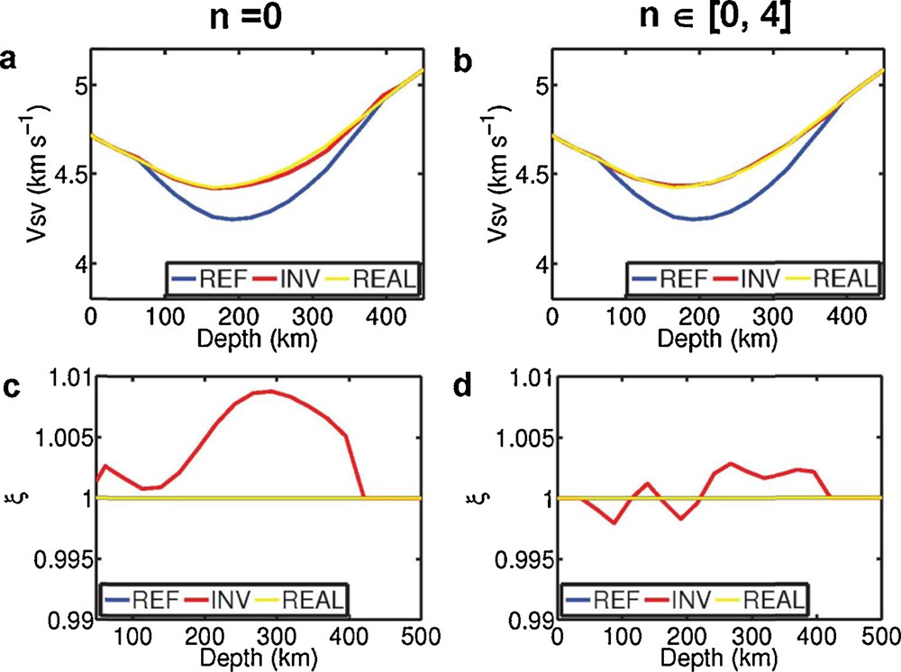
(Color online.) Inversion results of the 1066A model for the two groups of tests. The vertical S-wave velocity (VSV) for the first test (a) and for the second test (b), and the anisotropic parameter ξ for the first test (c) and for the second test (d), of the 1066A model (REAL), a perturbed reference isotropic model (REF), and the inverted model (INV). The dataset in the first test only contains the fundamental modes, and the dataset in the second test contains both the fundamental modes and the first four overtone modes.
We then derive two groups of tests. The dataset in the first group contains only fundamental modes, while the dataset in the second group contains both the fundamental and the first four overtone modes. The error bar of the phase velocity for the surface waves is set to be 1% for all of the tests in this paper. Also, we chose a diagonal matrix as the preconditioner to reduce the condition number of matrix in the linear equation system during inversion for all of the experiments, and we obtain the inversion results when the misfit is stable. Fig. 1 shows the inversion results of the most reliable parameters for surface wave data: the vertical S-wave velocity (VSV) and the S-wave radial anisotropy (ξ = N/L = V2SH/V2SV) (Dziewonski and Anderson, 1981) in these two tests. Fig. 1a, c give the velocity VSV and the anisotropic parameter ξ, respectively, of the reference, as the real and inverted models for the first test. Fig. 1b and d give the velocity VSV and the anisotropy parameter ξ of these models, respectively, for the second test. The VSV value for the inverted models of the two tests matches well the real model. For the radial anisotropy parameter ξ, its error in the first test is about 1%; and its error in the second test is about 0.2%. The errors of parameter ξ appear to be larger than those of VSV for both tests. One possible explanation here is that we can simply think that VSV (Fig. 1a, b) shows the absolute error of the S-wave velocity after inversion, while ξ (Fig. 1c, d) shows its relative error. Another reason is that the sensitivity of the Love wave (VSH) is not so good below a depth of 200 km. The inversion results are improved by the incorporation of additional information from the overtone modes in the data space during the inversion process. This is because the fundamental modes contain mostly information about the Earth upper mantle, whereas the first four overtone modes contain information about the Earth structure not only at shallow depths, but also at greater depths. These tests also illustrate that the theoretical errors produced by our phase velocity inversion method can be neglected (e.g., <0.2%) in the case when datasets contain enough frequency-band information.
We show the phase velocity differences of the Rayleigh and Love waves between the real model and the reference model before inversion for both the fundamental and the first four overtone modes (Fig. S1a, b), and between the real model and the inverted model of the first test for fundamental modes (Fig. S1e, f) and the second test for both the fundamental and the first four overtone modes (Fig. S1c, d). The phase velocities of the inverted models for both the Rayleigh and Love waves are similar to those of the real models in these two tests (Fig. S1c, d, e, f), and the phase velocity errors of the surface waves are within the error bars (given as 1%). Fig. S2 shows a comparison of seismograms for the vertical (Fig. S2a), radial (Fig. S2b), and transverse (Fig. S2c) displacement components for the reference model, the real model, and inverted models of the two tests for an example of an earthquake in Sichuan, China (latitude, 30.21°; longitude, 103.18°) in year 2013, at station 109C in California, USA (latitude, 32.889°; longitude, –117.105°; from the International Seismological Center website). The depth of this earthquake was 21.8 km, and the magnitude was Mw = 6.6 (from the CMT catalog; Dziewonski et al., 1981; Ekström et al., 2012). The epicentral distance of station 109C was 106.6°, and its back azimuth was 35.7°. The seismograms of the reference model and the real model are different for both the travel-time and amplitude, although the seismograms of the inverted models for both tests match well with those of the real model, which further illustrates the accuracy of our inversion method.
2.2 The isotropic PREM
The PREM is the most popular 1D reference Earth model (Dziewonski and Anderson, 1981). We chose the isotropic PREM to investigate the validity of our phase velocity inversion method in the presence of the Dirac's delta function-like large velocity contrasts and the mislocation of discontinuity.
2.2.1 The efficiency of the inversion method under a large velocity contrast
We use the isotropic PREM as the reference model (Fig. 2a), and we only consider the Dirac's delta function-like VS perturbation (β) of 3% (about an 85 m·s−1 constant perturbation) in the depth range of 80 km to 220 km, and of 4% (about a 180 m·s−1 perturbation) in the depth range of 220 km to 400 km. We also derive two groups of tests: one includes the fundamental mode in the dataset, and the other includes the additional first four overtones in the dataset. For both tests, the horizontal S-wave velocity (VSH) of the inverted models increases up to match well the real model, except for the discontinuities with large velocity changes (Fig. 2a, b). As surface waves do not see discontinuities in the Earth model well, we do not have that much information at the discontinuities in the dataset to help us recover the results at the discontinuities. However, by adding higher-order modes (overtones), the errors of the radial anisotropic parameter ξ of the inverted models are improved from about 1% (Fig. 2c) to about 0.2% (Fig. 2d), and they are relatively small even at the discontinuity with a large velocity contrast (Fig. 2d; e.g., the velocity difference at the discontinuity at the depth of 220 km is > 100 m·s−1). These small errors after inversion are mainly due to the combination of the filtering effect (or upscaling effect) and the limited frequency band of the dataset. This shows that our inversion method is accurate for Dirac's delta function-like perturbation on velocities for isotropic Earth models. The phase velocity of the inverted models also matches the real model relatively well, although the phase velocity difference between the real model and the reference model can be up to 200 m·s−1 (Fig. S3). The seismograms of the reference model and the real model are very different, especially for the travel-times, although the seismograms of the two inverted models fit that of the real model relatively well (Fig. S4).
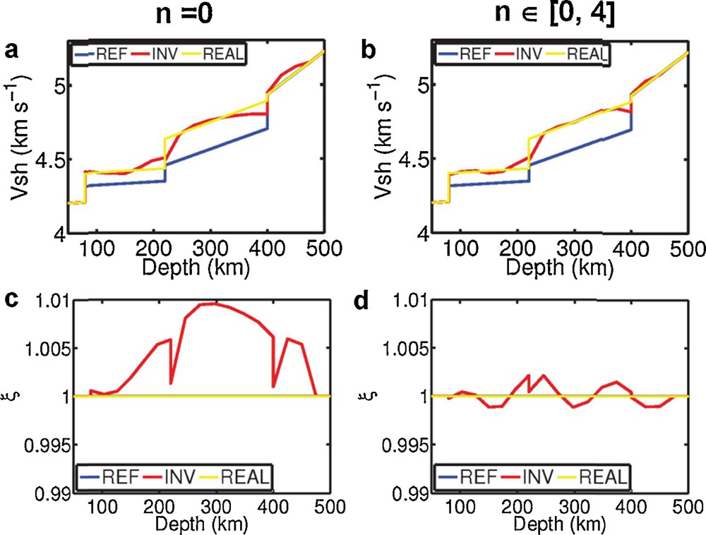
(Color online.) Inversion results of the isotropic PREM for the two groups of tests. The terms compared for the horizontal S-wave velocity (VSH) and the anisotropic parameter ξ are similar to those given for Fig. 1, but for the reference isotropic PREM (REF), the perturbed isotropic PREM (REAL) and the inverted model (INV).
2.2.2 The efficiency of the inversion method under the mislocation of the discontinuity
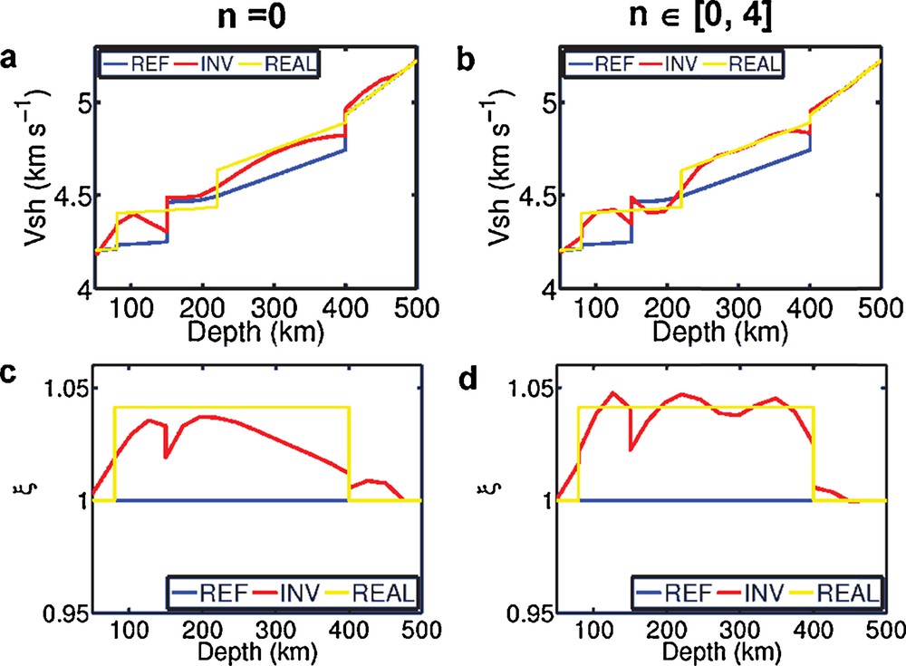
In this section, we investigate whether we can obtain accurate results when the depth of the discontinuity in the reference model does not fit that of the real model. What will the different results obtained for the velocity and anisotropy be in the presence of mislocation of the discontinuity? We choose the real model as for the test above (Fig. 2), and change the discontinuity of the reference model from the depth of 220 km to 150 km (Fig. 3a). As before, we use fundamental modes (Fig. 3a, c), and both fundamental and overtone modes (Fig. 3b, d) for the inversion. For these two tests, we find that except in the mislocation region (between the depths of 150 km and 220 km), the VSH of the inverted models increase well to approximate the real model, even though the VS contrast is about 150 m·s−1 between the depths of 80 km and 150 km, and about 160 m·s−1 between the depths of 220 km and 400 km (Fig. 3a, b). Moreover, in the mislocation region between the depths of 150 km and 220 km, the VSH of the inverted model decreases to reasonably approximate the real model (with the VS contrast about 80 m·s−1) for the second test (but not for the first test), due to the new information in the overtones. Unlike before, the radial anisotropy parameter ξ is not so accurate here, with errors around 0.5%, in spite of the addition of the overtone data. It shows that the incorporation of mislocation of the discontinuity can add large spurious anisotropy in tomographic models. However, the good agreement of both the phase velocity (Fig. S5) and the seismograms (Fig. S6) between the inverted models and the real model illustrates the validation of the phase velocity inversion results, especially for inverting anisotropy parameters.

(Color online.) Inversion results of the isotropic PREM with the mislocation of the discontinuity for the two groups of tests. The compared terms of the horizontal S-wave velocity (VSH) and the anisotropic parameter ξ are the same as those given for Fig. 1, but for a different reference PREM with a discontinuity depths change from 220 km to 150 km. The real model is the same as that given for Fig. 2.
2.2.3 The amount of extrinsic anisotropy at the discontinuity
For the upscaling effect, it is hard to define a general amount of extrinsic anisotropy at a discontinuity, as this is affected by the scale of the model and the seismic wavelength, the elastic properties of the layered model, and other effects. For the simple PITL model (Backus, 1962), the extrinsic radial S-wave anisotropic parameter ξ of its effective model can be calculated as:
| (1) |

Three types of isotropic layered models with small-scale heterogeneities: a: a three-layered model with a 20-km-thick low-velocity zone; b: a four-layered model with a 30-km-thick heterogeneity with both positive and negative velocity changes; c: a five-layered model with a 30-km-thick heterogeneity only with positive velocity changes.
Comparison of the amplitudes of the extrinsic S-wave radial anisotropy (ξ) at the discontinuities of the isotropic layered models with the vertical heterogeneities shown in Fig. 4. The comparison is between the homogenization method and the analytical solution (see Eq. (1)) of the effective model of the ‘equivalent’ periodic isotropic two-layered model.
| Case | Depth (km) | ξ Homogenization | Parameters for the equivalent PITL | ||||||
| p 1 | ρ1 (kg·m–3) | (km·s–1) | ρ2 (kg·m–3) | (km·s–1) | α | ξ PITL | |||
| A | 300 | 1.05163 | 0.80000 | 3.70 | 5.00 | 3.30 | 4.00 | 0.57081 | 1.05163 |
| 320 | 1.05163 | 0.20000 | 3.30 | 4.00 | 3.70 | 5.00 | 1.75189 | 1.05163 | |
| B | 310 | 1.08067 | 0.50000 | 3.70 | 5.00 | 3.30 | 4.00 | 0.57081 | 1.08068 |
| C | 295 | 1.00779 | 0.90361 | 3.10 | 4.00 | 3.30 | 4.50 | 1.34728 | 1.00780 |
| 303 | 1.01780 | 0.50000 | 3.30 | 4.50 | 3.50 | 5.00 | 1.30939 | 1.01828 | |
| 311 | 1.04140 | 0.36364 | 3.50 | 5.00 | 3.70 | 6.00 | 1.52229 | 1.04147 | |
| 325 | 1.14022 | 0.15730 | 3.70 | 6.00 | 3.10 | 6.00 | 0.37237 | 1.14023 |
Table 1 gives the comparisons of the amplitudes of the S-wave radial anisotropy parameter ξ at different discontinuities, between the homogenized effective model with a cut-off wavelength of 30 km and the effective model of the ‘equivalent’ PITL model for layered models (Fig. 4) in cases A, B and C, which can be calculated from Equation (1). The corresponding macro-scale parameter ɛ defined in the homogenization method (Capdeville and Marigo, 2007) is about 0.214 (ɛ = λcutoff/λmin = 30/(4 × 35) = 0.214, with minimum velocity Vmin = 4 km·s−1, and minimum period Tmin = 35 s, and thus the minimum wavelength of the wave-field λmin = Vmin × Tmin = 4 × 35 = 140 km). In case A (Fig. 4a), we show a low VS velocity zone (4 km·s−1) between the depths of 300 km and 320 km (thickness, 20 km). The other two isotropic layers are both with a high VS value of 5 km·s−1, and have a thickness of 80 km. The density in the second layer is 3.3 g·cm−3, and in the other two layers, 3.7 g·cm−3. The radial anisotropy at a depth of 300 km in case A for the homogenized model is 1.05163. Indeed, this is equal to the effective model of the equivalent PITL model with p1 = 80/(80 + 20) = 0.8 and α = μ2 μ1−1 = (3.3 × 42)/(3.7 × 52) = 0.5708, through Equation (1). The radial anisotropy at a depth of 320 km can be calculated the same way, and this is equal to that at the depth of 300 km. There is a 30-km-long heterogeneity in case B (Fig. 4b) between the depths of 295 km and 325 km. In this heterogeneity region, we create a 15-km-thick high-velocity zone with a positive velocity change, and a 15-km-thick low-velocity zone with a negative velocity change. The effective radial anisotropy parameter ξ at the discontinuity in this heterogeneous zone (at a depth of 310 km), as calculated by the homogenization method (ξ = 1.08067), is equal to that of the equivalent PITL model with p1 = 15/(15 + 15) = 0.5 and α = (3.3 × 42)/(3.7 × 52) = 0.5708.
In the 30-km-thick heterogeneity region of case C, we create three isotropic layers that all have positive velocity changes within the depths (Fig. 4c). The corresponding radial anisotropy at the discontinuities of this model can also be calculated through the effective model of the equivalent PITL model, and the details are given in Table 1. The other radial anisotropic parameters ϕ (which is related to the P-wave velocity anisotropy) and η of the effective model of the equivalent PITL model are also the same as those of the homogenized model at the discontinuities. Therefore, we have verified through these tests that for the isotropic layered model with scales much less than or equal to the seismic wavelength, we can ‘see’ it as an equivalent PITL model, and use the corresponding formulae to calculate the apparent radial anisotropic parameters at the discontinuity (Table 1).
Compared with the general homogenization method, the analytical solution (Eq. (1)) is very convenient and remains without loss of accuracy. We can apply this formula to study the amount of extrinsic anisotropy due to the upscaling effect for the isotropic layered petrological model in the upper mantle of the Earth (excluding the situation of partial melts here), where the shear modulus contrast α ∈ [0.7, 0.9] (assuming μ1 > μ2) (see Estey and Douglas, 1986) and p1 ∈ [0.3, 0.7]. Based on Equation (1), the effective S-wave anisotropy is ξ ∈ [1.0023, 1.0296]. We thus infer that the level of extrinsic S-wave anisotropy in the upper mantle of the Earth is within 3%, due to the vertical heterogeneities. As the radial anisotropy in reference Earth models such as PREM (Dziewonski and Anderson, 1981) is usually stated as being about 10%, we estimate that the extrinsic anisotropy in the upper mantle might be up to 30%.
2.3 The anisotropic PREM
The radial anisotropy was introduced in PREM to explain the discrepancy between the eigenfrequencies of spheroidal and toroidal modes equivalent to Rayleigh and Love waves, and body-wave travel-times (Dziewonski and Anderson, 1981). In this part, we choose an anisotropic PREM between the Moho and the 220-km discontinuity, to investigate the accuracy of our inversion method in the presence of large velocity and anisotropy contrasts, and the mislocation of discontinuity.
2.3.1 The efficiency of the inversion method under a large velocity contrast
Start from a reference isotropic PREM (Fig. 2a), we give the VSV and VSH have a β = 3% perturbation between the depths of 80 km and 220 km, and give only the VSH has a β = 3% perturbation between the depths of 220 km and 400 km (Fig. S7a). So there is a Dirac delta function-like perturbation for anisotropy parameter ξ between the depths of 220 km and 400 km, and for the VSH between the depths of 80 km and 400 km. The amplitude of ξ in the ‘real’ model is about 1.061 between the depths of 220 km and 400 km (Fig. S7c, d).
As before, we carry out two groups of tests that depend on whether the first four overtone modes are incorporated or not in the inversion process (Fig. S7). After several iterations, the VSH for both cases are accurately retrieved, except at discontinuities, although the perturbation for VSH reaches about 100 m·s−1 to 200 m·s−1. For the anisotropic parameter ξ, we obtain good results for the test with the overtones included in the dataset (Fig. S7d), while the test just with the fundamental mode is not as good (Fig. S7c), as the sensitivity of Love waves is very poor below the depth of 150 km for this anisotropic PREM (with an error of about 2%). This illustrates that we can obtain a better result if more information is considered during the inversion, such as higher-order modes in the dataset. This also illustrates that intrinsic anisotropy is more difficult to be retrieved when we add a perturbation to the anisotropy parameter, compared with the results of the isotropic PREM test with a perturbation only on the velocity (e.g., Fig. 2c, d, Fig. 3c, d, at a depth of 220 km). However, from the comparisons for both the phase velocity (Fig. S8) and the seismograms (Fig. S9) between the real model and the inverted models, we can still trust these inversion results under large perturbations for both the velocity and the anisotropy parameters. The large errors at the discontinuities arise because the normal modes and the surface waves cannot see step functions, but only filtered parts of discontinuities. This is also because we search for the solution in the L2 norm space, which will not have good resolution at the discontinuity for a Dirac's delta function-like perturbation. Thus, the tomographic model we find after the inversion is usually an upscaled (homogenized) model of the ‘real’ Earth model, as demonstrated in Capdeville et al. (2013) for full waveform inversion.
2.3.2 The efficiency of the inversion method under the mislocation of the discontinuity
Similar to the isotropic PREM case with mislocation of the discontinuity (Fig. 3), we decrease only the VSV of the real PREM in Fig. 3 to change it into an anisotropic PREM (Fig. 5), and we keep the reference PREM unchanged. By adding the first four overtone modes during the inversion, we improve the results for both the VSV and the anisotropic parameter ξ, except at the discontinuities with large velocity contrasts (Fig. 5). The correlation length in the covariance matrix Cp is chosen as 50 km. In the mislocation region (between the depths of 150 km and 220 km) for the second test, the VSV of the reference model decreases to fit the real model even under a velocity contrast of about 120 m·s−1, and the radial anisotropy parameter ξ increases from 1.0 in the reference model to 1.041 in the real model, except at the discontinuity at the depth of 150 km (Fig. 5b, d). As high frequency data is lost in the surface wave data at the depth of 150 km, where a mislocation of the discontinuity lies, it is hard for us to find a ‘true’ model there when we minimize the misfit function. The inverted model with large spurious anisotropy at the depth of 150 km is actually the ‘homogenized’ model due to the upscaling effect. However, the comparisons for both the phase velocity (Fig. S10) and the seismograms (Fig. S11) between the real model and the inverted ones still illustrate the effectiveness of our inversion method.
(Color online.) Inversion results for the anisotropic PREM with a mislocation of the discontinuity for the two groups of tests. The compared terms are the same as those in Fig. 1, but for the vertical S-wave velocity (VSV) and the anisotropic parameter ξ. The mislocation region is in the depth range between 150 km to 220 km. The reference model is the same as that given for Fig. 3.
2.4 The PREM with the incorporation of crustal models
In this section, we design two isotropic PREM to consider the impact of the incorporation of crustal models with the upper mantle models on the inversion results when we try to fit the dataset (Bozdağ and Trampert, 2007; Ferreira et al., 2010). We choose two isotropic PREM with velocity perturbation (Fig. S12) and mislocation (Fig. 6) in the crust and the upper mantle, which are modified from models in Figs. 2 and 3, respectively. We perform two groups of tests for each model. One interesting result is that by the addition of the overtone modes, we do not improve the inversion results as before, but get some oscillations in the upper mantle when the crust model with mislocation is added. Also, the extrinsic radial anisotropy is up to 2% (Fig. 6 and Figs. 6d and S12d), because the crust model usually has large velocity contrasts at discontinuities, and thus a large impact on the misfit function compared with that of the upper mantle model. Therefore, we obtain a biased model when we try to minimize the overall misfit, which might misguide the interpretation of the seismic anisotropy.
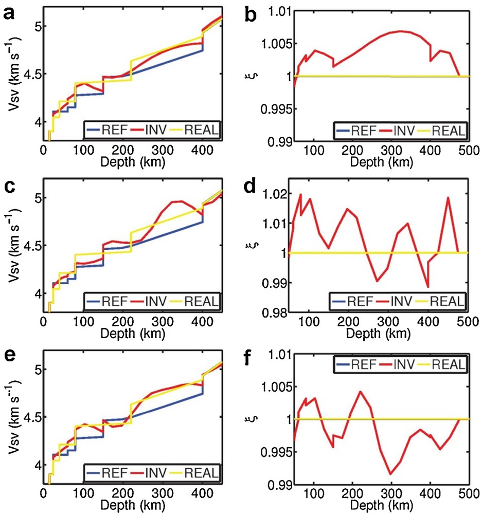
(Color online.) Inversion results of the vertical S-wave velocity (VSV) (a, c, e) and the anisotropic parameter (ξ) (b, d, f) of an isotropic PREM with mislocations of discontinuities for three groups of tests. The dataset in the first test contains just the fundamental modes, while in the second and third tests they contain both the fundamental and the over tone modes. The starting model in the first and second tests are the same, while the third test is the inverted model of the first test. The mislocation regions are between the depth range from 25 km to 80 km and 150 km to 220 km.
However, by comparing Fig. 6a with Fig. 6c, we indeed improve the results in the mislocation regions when the overtone modes are incorporated. Thus, we propose to first use fundamental modes to get a ‘stable’, and almost ‘fit’, model, and then to add overtone modes for the second step inversion starting from the inverted model in the first step. In this way, we indeed improve the results in the third group of tests of VSV at the discontinuity of 400 km (Figs. 6e, S12e), and the error of the radial anisotropy ξ (Fig. S12f). Also, as shown in Fig. 6e, we recover the resolution in mislocation regions especially for the velocity parameter VSV using this strategy. For radial anisotropy in the mislocation model (Fig. 6f), we still need to add more information to the dataset (e.g., a wider period band) to further improve its resolution at discontinuities. We infer this strategy might also be used when the velocity or anisotropy perturbation in the model is very large, and even a little bit beyond the scope of the first-order perturbation theory.
3 Conclusions and discussion
The inversion method usually brings artificial anisotropy to the inverted model, mainly due to the lack of information in the seismic data, which will bias the interpretation of the anisotropy in the seismic data. Different linear and nonlinear inversion methods have been discussed here. We propose an iterative surface wave-phase velocity-inversion technique based on first-order perturbation theory, to try to better recover the information in the surface wave phase velocity dataset. The corresponding forward problem (for the calculation of the phase velocity) is calculated by normal mode theory. We then use the iterative quasi-Newton method to minimize the classical least-square cost function, with damping on both of the data and model parameter spaces, and choose the GMRES method to solve the linear equation during the inversion process, because of its accuracy and numerical stability.
When inverting a continuous perturbation (Fig. 1) or a Dirac delta function-like perturbation (Figs. 2, 3, 5 and Figs. 2, 3, 5, S7) on the VS and radial anisotropic parameter ξ, we obtain accurate results using our iterative quasi-Newton method together with the GMRES method. In particular, the results for the continuous 1066A model illustrate that the extrinsic anisotropy produced by the theoretical errors of our surface wave phase velocity inversion technique can be neglected. The extrinsic anisotropy in tomographic Earth models is thus mainly due to the filtering effect, the limited frequency band in the dataset, or the bad quality of the data coverage.
For the isotropic cases (i.e., the continuous 1066A model or the PREM with several discontinuities at different depths), the error of the radial anisotropy parameter ξ is within 0.2% (Figs. 1 and 2), even though the velocity contrast can be as large as several hundreds of meters per second. For the isotropic or anisotropic PREM with mislocation of discontinuities, the error for the S-wave anisotropy (ξ) at the discontinuities is larger than that for other continuous parts of the model (where the error of ξ is about 0.5%), even when using higher modes during the inversion (Figs. 3d, 5d). This is because, as discussed before, the surface waves do not see the details of the discontinuities of the Earth, and what we get is usually the homogenized model. To further improve the inversion results at the discontinuity, we can use a wider period band during inversion. More efficiently, we can combine our phase velocity inversion method with the joint inversion of receiver functions that contain high-frequency data (Bodin et al., 2012; Julia et al., 2000) that are not included in the surface wave data. We suggest that more kinds of data, such as receiver function data (Bodin et al., 2015) or P-wave data (Fichtner et al., 2013), should be incorporated to distinguish intrinsic anisotropy from extrinsic anisotropy in tomographic Earth models.
The incorporation of the mislocation of the discontinuities in the crust will add instabilities during the inversion when we try to use higher overtone modes to improve the resolution (Fig. 6). We have illustrated here that one effective solution is to get a ‘stable’ inverted model using only fundamental modes first. Then, we start with this model, and use both fundamental and overtone modes to obtain the final improved result. We propose that another possible solution is to use a homogenized model with no discontinuity as the starting model. The de-homogenization needs receiver functions or body-wave data to correctly locate the discontinuities.
The extension of the Backus long wavelength equivalent theory to the general layered isotropic model (which is not necessarily a periodic model) with spatial scales less than or equal to the seismic wavelength (Table 1) might also provide us with information for the investigation of the mechanism of seismic anisotropy. For radial anisotropy, we derived the stable long wavelength equivalent region (SLWER) tests based on the PITL model (related to fine layering) to explore the mechanism of radial anisotropy in PREM (Wang et al., 2013). In the isotropic PREM section, we discussed how there can be up to 30% extrinsic radial anisotropy of the 10% observed radial anisotropy in the upper mantle of the Earth. The additional information of the azimuthal anisotropy (parameter and its azimuth from the surface wave; δt and ϕ from shear wave splitting [SKS] of the body wave) can further help us to investigate the origin of the apparent anisotropy. For example, Song and Kawakatsu (2012) proposed that a tilted layered model plus intrinsic LPO can help to explain the SKS splitting data in oceanic subducted slabs. We propose that using the analytical tool of Backus theory (Backus, 1962), the simple tilted PITL model can provide a way to explore both radial and azimuthal anisotropy for such as oceanic subducted slabs, to help us to discriminate between extrinsic and intrinsic anisotropy. In this way, we might be able to explain the discrepancy between radial and azimuthal anisotropy in real seismic data, such as that in surface wave data and body-wave data.
We should note that for the inversion technique, we have mainly concentrated on the 1D surface wave phase velocity inversion method and have inverted for VTI models (with five radial parameters). We can extend this easily to the 3D case and to more general anisotropic models by adding more degrees of freedom in the model parameter space (e.g., by adding eight azimuthal terms of a slight anisotropic medium; Montagner and Nataf, 1986) and by adding the corresponding sensitivity kernels of the data space with respect to the model parameters (see Appendix B). For the numerical stability and accuracy of the GMRES method, we expect reliable results from its application to real surface wave phase velocity data, to image both regional and global tomographic Earth models, and to help us to better understand the mechanism of anisotropy and the related geodynamic processes of the Earth. Moreover, shorter period band of phase velocity data can be included to image the crustal structure of the Earth, and longer period bands of phase velocity data can also be considered to investigate the anisotropy structures in the deep Earth, such as the transition zone and the D″ layer.
Acknowledgements
This work was supported by European I.T.N. QUEST and ANR Blanc “mémé” (ANR-10-Blanc-613). The authors would like to thank Editor Michel Campillo, and the two reviewers Andrea Morelli and Yanbin Wang for constructive comments that helped to improve the manuscript. We would also like to thank Daniel Clarke, Florian Duret, Gaye Bayrakci, Haiyang Wang, James Martin, Jean-Pierre Vilotte, Laurent Guillot, Pierre Dublanchet, and Xinchun Yu for discussions.