

1 Introduction
In recent years, the use of seismic ambient noise correlations pioneered by Shapiro and Campillo (2004) have opened up new ways to obtain high resolution images of the crust (Sabra et al., 2005a; Shapiro et al., 2005). In particular, in many regions, such images could not be obtained using conventional methods that use seismic waves emitted by earthquakes because of insufficient coverage provided by such data.
The principle of passive imaging is that the correlation of a random wavefield recorded by distant receivers contains the complete Green function of the medium including all propagation modes (Weaver and Lobkis, 2001). This gives the possibility to perform measurements of the seismic wave travel times between any pair of receivers. These measurements can then be inverted to image the Earth’s interior.
This result, as established theoretically (e.g. Colin de Verdière, 2006; Weaver and Lobkis, 2001), is valid in any medium but relies on a strong assumption: the wavefield has to be equipartitioned: all modes of the medium have to be excited with the same level of energy and with a random phase (Sánchez-Sesma and Campillo, 2006). Equipartition is achieved for instance if there are white noise sources everywhere in the medium (Colin de Verdière, 2006) or if a few sources are present in a highly scattering medium. Alternatively this result can be established by invoking the stationary phase theorem (Roux et al., 2005b; Sabra et al., 2005b; Snieder, 2004), the fluctuation-dissipation theorem (Godin, 2007; van Tiggelen, 2003) or the reciprocity theorem (Wapenaar, 2004; Wapenaar et al., 2006).
In seismology, the term “ambient noise” refers to all elastic waves propagating through the Earth that are not generated by earthquakes or explosions. Indeed, the Earth undergoes continuous oscillations that are related to the interaction between the ground, the ocean and the atmosphere. At periods larger than 1, even averaged over one year, the distribution of noise sources at the surface of the Earth is not homogeneous and does not match completely the requirement of the theory that relates noise correlations to the Green function of the medium (see, for instance, Chevrot et al., 2007; Kedar et al., 2008; Landès et al., 2010; Rhie and Romanowicz, 2004; Stehly et al., 2006; Stutzmann et al., 2009; Yang and Ritzwoller, 2008)
1.1 Current limitations of ambient noise tomography
The uneven distribution of noise sources, the fact that one uses a finite amount of data to compute noise correlations, and the way noise correlations are inverted implies several limitations on ambient noise tomography:
- (i) In typical regional tomographic studies such as Shapiro et al. (2005) or Stehly et al. (2009), less than one interstation path out of three is used. Other paths are rejected because either surface waves cannot be identified unambiguously, or the surface wave travel times measured on the positive and negative side of the correlation are not consistent. This is mostly due to the uneven distribution of noise sources;
- (ii) The full Green function is not reconstructed: usually only the surface wave fundamental mode emerges from the correlations. In particular, body waves have only been observed in particular situations (Draganov et al., 2009; Roux et al., 2005a; Zhan et al., 2009) and are not yet commonly used for tomography;
- (iii) The velocity of surface waves can be systematically over or under estimated in certain azimuth since noise sources are not evenly distributed (Tsai, 2009; Weaver et al., 2009). This could be erroneously interpreted as anisotropy of the medium;
- (iv) Most of the time, surface wave dispersion curves are inverted using ray theory that is strictly valid only at infinite frequency and does not account for the complexity of wave propagation within the 3D Earth. This is particularly problematic for the crust which can be extremely heterogeneous.
1.2 A possible way to challenge these limitations
Ideally one could overcome these limitations – at least partially – by designing an efficient denoising filter to extract the signal corresponding to the Green function from the random fluctuations of the correlations, and taking into account the distribution of noise sources when inverting noise correlations. “Denoising” noise correlations would make it possible to identify surface waves and eventually other propagation modes reliably on a larger number of paths. Computing synthetic correlations by simulating a realistic distribution of noise sources using the spectral element method (SEM) (Komatitsch and Vilotte, 1998) would eliminate most of the biases arising from the uneven distribution of noise sources during the forward problem. For this purpose, we will use Spectral Element Method (SEM) (Komatitsch and Vilotte, 1998) rather than other methods such as an approach based on normal mode summation (Cupillard and Capdeville, 2010) because it will ultimately allow us to perform simulations in arbitrary 3D structure, without restriction on the velocity contrasts or wavelengths of heterogeneity.
We will see that these two points are closely related: the capability to “denoise” noise correlations is essential for the computation of accurate synthetic correlations which, in turn, makes it possible to identify surface waves on correlations based on real data, even when the signal to noise ratio is low.
These ideas are simple but lead to a practical question: is it really possible to obtain synthetic correlations in a reasonable computational time by simulating directly an ambient noise wavefield ? More precisely, how long a data record do we need to get a reliable correlation? In real applications one typically uses records that are up to several years long. Simulating such long time series to high frequency (up to 0.2Hz) using the SEM at the global or large regional scales is out of question because the computation would take several years on a modern cluster!
To answer this question we implement seismic noise sources within RegSEM, a regional spectral element code (Cupillard et al 2011, submitted). In Section 2 we demonstrate that it is possible to compute synthetic correlations by simulating a random wavefield but that it requires several months of data. We show in Section 3 that using curvelet filters allows a faster and more accurate Green function reconstruction. A few days of noise data are then sufficient to retrieve the full Green function including overtones. Finally we show in Section 4 that synthetic correlations can in turn be used to identify surface waves in a reliable manner on noise correlations even if their signal to noise ratio is much lower than one.
2 Simulating seismic ambient noise using the spectral element method
Our aim is to probe the possibility to compute synthetic noise correlations by introducing noise sources in RegSEM (Cupillard et al 2011, submitted) a regional spectral element code.
We start by investigating the easiest case, that is a homogeneous distribution of random noise sources located at the free surface of an attenuating and spherically symmetric Earth model. Our simulation consists of 37 numerical runs computed in PREM (Dziewonski and Anderson, 1981) with attenuation and lasting 4 000 s. We consider a 75x35 degree wide region surrounded by absorbing boundaries (the so-called PML (Festa and Vilotte, 2005)), spanning the upper mantle down to 600 km depth. During each numerical run we impose a random vertical traction that is continuous in time and space at the surface of the Earth. This generates a random wavefield that mimic seismic ambient noise.
An array of 40 × 5 receivers separated by 60 km records the vertical displacement (Fig. 1). We retrieve the Green function between each station pair by taking the time derivative of the correlation of the background seismic noise records. For the rest of this article, we will always compare the time derivative of the correlation with the Green function of the medium. No processing is performed on the noise records, such as frequency whitening or one-bit normalization.
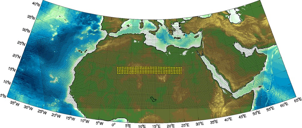
Map showing the stations (yellow triangles) and the grid (black dots) used for the numerical simulations.
Carte des stations utilisées lors des simulations numériques de bruit.
Since we consider a 1D model, the Green function depends only on the source-receiver distance. This implies that all correlations computed between station pairs separated by the same distance converge towards the same Green function. Therefore we consider that averaging the correlations over time or over station pairs is equivalent: correlating T seconds of noise between two stations yields a similar result as summing N correlations of T/N seconds computed between N stations pairs separated by the same distance. Since we performed 37 runs of length 4000 s, each receiver has recorded 37 ∗ 4000 s = 1.7 days of noise. As we have, for instance, 140 pairs of stations separated by 720 km, summing the corresponding correlations we will obtain a similar result as if we correlated 37 ∗ 140 ∗ 4000 s = 237 days of noise on one pair of stations. This is particularly convenient to study how the correlations converge towards the Green function.
This is, however, only an approximation that would be perfectly valid only if the signals recorded by all the receivers were completely independent of each other. This assumption is not completely fulfilled in our case, since we use a regular grid of stations separated by 60 km to study surface waves whose wavelengths range from 60 to 240 km.
Figure 2 shows a comparison of the Green function (black line) and the noise correlation (blue dashed line) computed between stations separated by 720 km in the 20–40 s period band. When using only one day of noise, surface waves are already visible on the correlation time series with a correct arrival time. However, the signal to noise ratio remains low: large fluctuations, that are not a part of the Green function, are visible in the correlation time series before and after the surface wave. Without knowing the Green function, it would be hard to tell if these fluctuations are meaningless or if they are real arrivals due to effects of 3D structure such as, for example, multipathing. When correlating a larger length of noise record, these fluctuations become less important, and finally with 200 days of noise the correlation is close to the Green function.

Comparison between the Green function (black) and the correlation (dotted blue) of 1,10 and 200 days of noise computed between two stations separated by 720 km. All traces are filtered in the 20–40 s period band.
Comparaison entre fonctions de Green et corrélations de bruit synthétiques.
The bottom line of this section is that: (1) it takes only a few days to reconstruct accurately the surface wave part of the Green function (Fig. 2); and (2) several months of data are required for the random fluctuations of the correlation to disappear (Fig. 2). This leads to a fundamental point : if most of the information on the medium is already present on a correlation averaged over a few days, then it should be possible to isolate this information from the random fluctuations of the correlation. This would allow us not only to measure more accurately the surface wave travel times, but also to reconstruct the full waveform of the Green function using a smaller record length. We address this in the next section.
3 Improving synthetic noise correlations using curvelet filters
Our goal is to separate the information on the medium that is present in the correlations from the pseudo-noise that does not belong to the Green function. Let us see how this can be done with an example.
Our input signal C is a matrix containing 128 correlations of 1000 s with a sampling rate of 5 s computed between stations separated by 720 km (Fig. 4a). We do not see any signal on these correlations since correlating 1000 s of noise is not sufficient to reconstruct the Green function with an acceptable signal to noise ratio (SNR). However on the sum of the 128 correlations, the Rayleigh wave is visible but with low signal to noise ratio (Fig. 4a lower panel).
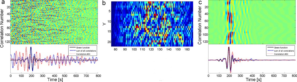
a) Matrix of 128 correlations of 1000 s of noise computed between two stations separated by 720 km. Lower panel: Green function between the two stations (black), the sum of the 128 correlations (dashed blue line, surface waves are visible with a low SNR), and the correlation #60 (red line, we do not see any signal). We show only the positive time of the correlations. b) Coefficients of the curvelet transform cj=3(x, y). c) same as a) after the correlation matrix has been denoised using curvelets.
Comparaison d’une matrice de corrélations de bruit synthétiques brute et débruitée.
In the case where noise sources are homogeneously distributed we have
| (1) |
It turns out that the curvelet transform is particularly well suited for our purpose (Candès et al., 2006). Curvelets are designed to represent images at different scales and angles. Like the wavelet transform, it is a multiscale transform, but it uses a basis of functions that are simultaneously localised in frequency, in physical space1 and in orientation. Frame elements are indexed by their level or scale j, angle θl, and x, y position. In physical space, they look like little plane waves having different orientations, that oscillate in one direction and are smooth in the perpendicular direction (Fig. 3b).
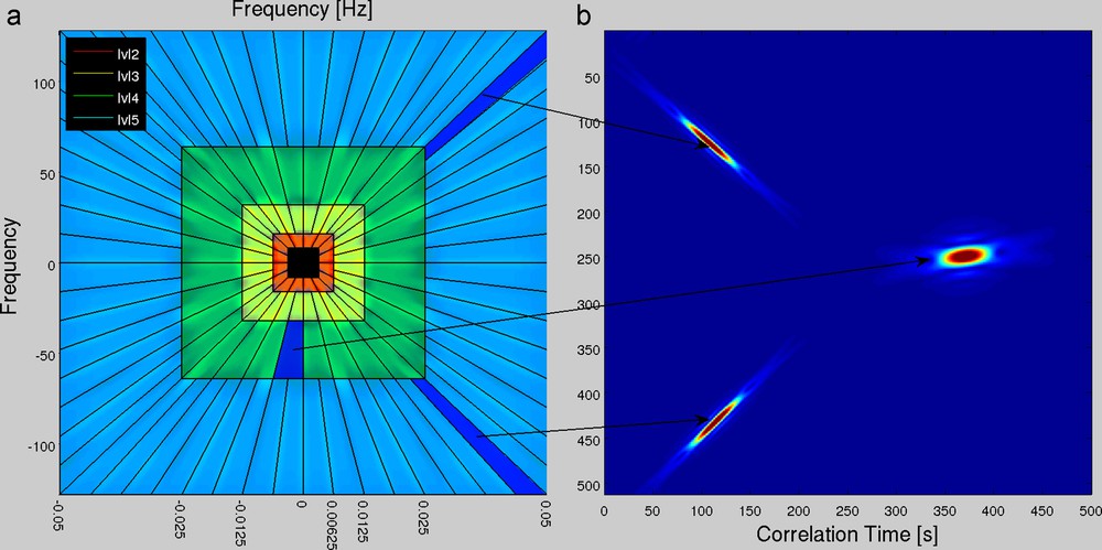
a) Curvelets are constructed in the frequency domain by tiling the frequency plane with trapezoids: the inverse fourier transform of each wedge is a curvelet in the physical space having a particular scale and orientation. Furthemore curvelet can be translated along the x and y axis. All curvelets of the same scale lie on the same ring in the frequency domain. We show curvelets of level 2,3,4 and 5 respectiveley in red, yellow, green and blue. b) Curvelets frame elements are indexed by their level (scale) j, angle θl, and position x, y. Here we show two curvelets in physical space of level 5 (left) and one curvelet of level 4 (right). Each of these curvelets was obtained by taking the inverse fourier transform of the wedge indicated with an arrow.
Construction des curvelets.
In a nutshell, curvelets are obtained by tiling the frequency plane with trapezoids as shown on Fig. 3a. The 2D inverse Fourier transform of each wedge, i.e of a function whose absolute value is close to one within the wedge and vanish outside, defines a curvelet. All wedges located on the same ring define curvelets having the same level (scale) and different orientations in the physical space (Fig. 3b). Furthemore, curvelets can be translated along the x and y axis in the physical space. Curvelets provide an optimally sparse representation of objects with edges and wave propagators (Candès and Demanet, 2004). For this reason, the curvelet transform is an ideal choice for detecting wave fronts and suppressing noise in seismic data (Herrmann et al., 2007) and, as we shall see, in the noise correlation matrix.
Since we are going to use curvelets to represent the matrix C whose each row is a correlation, in our case the x-axis of the physical space will be the correlation time in seconds. The correlations have a sampling rate of 5 s, and most of their energy is between 20 and 100 s of periods. So in the curvelet domain, most of the energy will be between level 3 and 5 (Fig. 3a).
Let cj,l(x, y) and gj,l(x, y) be, respectively, the coefficient matrices of the curvelet transform of C and G (the signal we want to extract from C) at level j, angle θl, and discrete position x, y (Fig. 4b). As we mentioned earlier, the rows of G are identical since they are all the Green function of the medium. This has two consequences: (1) gj,l(x, y) does not depend on y; (2) in physical space, we look specifically for a zero-angle (vertical) signal. So we project C at each level j and position x, y only on vertical curvelets. We threshold the coefficient, that is we keep only the highest coefficients of cj,l(x, y), and bring the data back in the physical space.
The result is shown on the Fig. 4c. On each row of the matrix, i.e on each correlation, Rayleigh waves are now clearly visible around 200s. The sum of all correlations (Fig. 4c lower panel) has also been improved and has a similar waveform as the Green function (black line). This example illustrates how it is possible to successfully extract the Green function from a correlation having a moderate signal to noise ratio. Let us quantify more precisely what are the benefits of the curvelet filter.
3.1 Comparing raw and denoised correlations
In Fig. 5 we compare Green functions (solid line) with raw and denoised correlations (dashed line) computed using 1.5 and 11 days of noise between stations separated by 360, 720 and 1440 km. For each comparison, we indicate the travel time difference dt of surface waves measured on the Green function and on the correlation at periods between 25 and 60 s, as well as the waveform misfit defined as
| (2) |
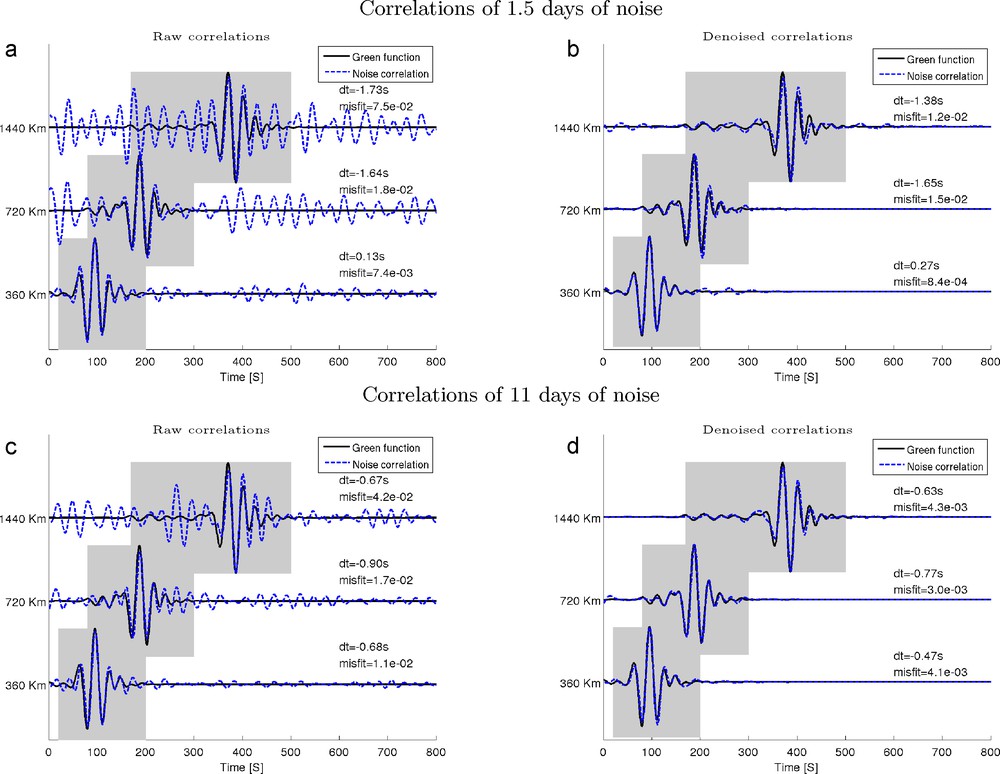
a) Correlation of 1.5 days of noise between stations separated by 320, 720 and 1440 km (dashed line) vs the Green function between the same stations (solid line). b) same as a) but the correlations were denoised using curvelets. c, d) same as a,b) except that 11 days of noise are used to compute the correlations. For each comparison, we show the misfit of the correlation and Green function waveforms measured in the shaded area, and the surface wave travel time difference dt.
Exemples de corrélations de bruit, brutes et débruités.
It is clear on all examples shown that curvelet filters successfully isolate the signal from the random fluctuations of the correlations. For instance, at 1440 km, we see higher modes on the Green function around 250 s that are absolutely not visible on raw correlations (Fig. 5c). However, these higher modes appear more clearly on denoised correlations especially when using 11 days of noise (Fig. 5d). This illustrates that curvelet filters make it possible to retrieve the Green function’s waveform more accurately, and to identify other arrivals than the surface wave fundamental mode. Hence the waveform misfits are much lower on denoised correlations than on raw correlations. The improvement can be up to one order of magnitude (at 360 km with 1.5 days of noise for instance, Fig. 5b). On the other hand, denoising correlations do not improve significantly Rayleigh wave travel time measurements. This is consistent with what we have seen in Section 2: travel time measurements of the Rayleigh wave are already reliable when correlating a few days of noise, and cannot really be improved.
We have seen that thanks to the curvelet filter, simulating 1.5 days of noise is sufficient to retrieve accurately the waveform of the surface wave part of the Green function with a high signal to noise ratio. Higher modes can be obtained using 11 days of noise. It is therefore practically possible to compute accurate synthetic correlations by simulating directly ambient noise sources using the spectral element method – at least in a 1D Earth model.
4 Using curvelets to denoise correlations having an SNR ≪1 using a “reference correlation”
We have seen in the previous section that curvelet filters make it possible to compute accurate synthetic correlations by simulating less than three days of seismic noise which requires less than one month of computation time on a small cluster (at periods greater than 20 s). We want now to show that one can use the curvelet transform in a different way to extract the Green function of the medium from a matrix of noise correlations C whose signal to noise ratio is much lower than one. This method is more efficient than the one presented in the Section 3, but it assumes that one has a “reference correlation” that is close enough to the actual Green function of the medium. When addressing a tomographic problem, the “reference correlation” could be a synthetic correlation computed in an initial Earth model as shown in the previous section that is used to denoise correlations of real data.
We start with a matrix C of 256 synthetic correlations of 1000 s of noise computed in PREM and recorded by two stations separated by 720 km to which we add some white noise filtered between 20 and 80 s, whose amplitude is 6 times larger than that of the data (Fig. 6a and b). The signal to noise ratio of the correlations is much lower than one. No signal is visible even on the sum of all the 256 correlations (Fig. 6b lower panel). Is it possible to extract any signal from these data?

a) Top panel: 256 correlations of 1000s of noise computed between two stations separated by 720 km. Lower panel: the sum of all correlations. b) Same as a) but we added to each individual correlation white noise whose amplitude is 6 times greater than that of the data. The signal to noise ratio of the sum of all correlations is much lower than 1 s. Surface waves are no longer visible on the sum of all correlations (lower panel). c) Matrix of reference correlation that is used to construct the curvelet filter. d) We use the reference correlation shown in c) to construct a curvelet filter that allows us to denoise the correlations shown in b). The denoised correlation is shown in blue and is compared to the Green function in red.
Utilisation d’un signal de référence pour débruiter une matrice de corrélations dont le rapport signal sur bruit est inférieur à 1.
We proceed in two steps. Firstly, we demonstrate that it is possible to isolate the signal of C from the noise in the curvelet domain if one already knows the green function of the medium. Secondly, we show that this result still holds if instead of the exact green function one use a “reference correlation” that is significantly different from the Green function.
4.1 Using the Green function of the medium to extract the signal from the noise of C in the curvelet domain
To extract the signal from C, we construct a matrix G having the same size than C, whose each row is the green function of the medium (Fig. 6c). We then multiply the coefficients of the curvelet transform of C by those of G rescaled between 0 and 1, and bring the data back into the physical space. This is a simple way to window the signal of C in the curvelet domain. The result is shown on the Fig. 6d. We now see clearly surface waves with an arrival time of about 200 s on the correlation matrix. The sum of all correlations shown on the lower panel has a waveform that is close to the exact Green function of the medium. In particular, the surface waves of the Green function and the denoised correlations have the same arrival time, whereas they could not even be identified on the original correlation.
Of course, in practice, it is perfectly useless to use the Green function to extract … the Green function from C! But this shows that in the curvelet domain, the signal of C can be isolated from the noise. These properties is related to the fact that the curvelet transform provides an optimally sparse representation of the solution of the wave equation in smooth mediums.
4.2 Extending this method by using a “reference correlation” rather than the Green function of the medium
Now let us see what happens if one uses a “reference correlation” instead of the Green function of the medium to extract the signal from C. In our case the reference correlation is assumed to be simply the exact Green function of the medium shifted by either 0, 10, 25 or 50 s as shown on Fig. 7. For each of these reference correlations, we attempt to extract the Green function from C using the procedure presented in the previous section. The result is presented on the Fig. 7. We see that as long as the reference correlation is shifted by less than 25 s with respect to the Green function (that is the half of the dominant period of the signal), the signal extracted from C (dotted blue) is close to the green function of the medium. In particular the arrival time of the fundamental mode of the surface waves are identical. However, when the “reference correlation” differs strongly from the Green function, it is no longer possible to use it to denoise C (see Fig. 7 for dt = 50 s): the denoised correlation differs strongly from the green function, and it becomes difficult to measure the arrival time of the surface wave.

We compare the sum of the denoised correlations matrix (Fig. 6b) in dotted blue and the Green function of the medium (black), when different reference correlations (red) are used to construct the curvelet denoising filter. As long as the travel time of the surface waves of the reference correlation differs by less than half a period (dt = 25 s) from the GF, it can be used to construct a curvelet filter that can be applied to a noisy correlation to extract the Green function of the medium.
Influence du choix du signal de référence.
4.3 Conclusion
The bottom line is that as long as the travel time of the surface waves of the reference correlation differs by less than half a period (dt = 25 s) from the Green function, it can be used to construct a curvelet filter that can be applied to a matrix of correlations having a signal to noise ratio lower than one, to extract the Green function of the medium from them. This is particularly interesting, as in typical tomographic studies at the continental scale, more than two thirds of the correlations are discarded, since it is not possible to make reliable travel time measurements. We hope that this method will be useful to include more measurements and eventually identify other arrivals than surface waves, and thus provide additional constraints on tomographic models.
However there is no magic! First, this method works only provided that the surface wave travel time on the reference correlation and the Green function do not differ by more than half a period. Second, a correlation can be “denoised” only if it contains deterministic information about the medium. This is ensured in our synthetic tests by the homogeneous distribution of noise sources at the free surface. Applying this to real data may be harder since real noise sources are not evenly distributed. One may have to use synthetic correlations computed with a realistic distribution of noise sources to denoise real correlations. This means that noise sources may have to be located accurately first. This may be a challenge!
5 Discussion and conclusion
The aim of this article was to investigate a possible way to improve ambient noise tomography. We used the spectral element method to simulate a homogeneous distribution of noise sources at the free surface of a layered Earth (PREM). We have shown that several months of data are required for the correlations to converge towards the Green function of the medium (Fig. 2). On the other hand, hopefully there are already deterministic informations on the medium on a correlation averaged only over a few days (Fig. 2). By using a curvelet filter, without any a priori, it is possible to extract this information from the random fluctuations of the correlation. With this method, simulating less than two days of data is enough to retrieve surface waves accurately from noise correlations, and using about 10 days of data one can also distinguish higher modes (Fig. 5).
This shows that it is possible to use the spectral element method to compute synthetic correlations and Green functions by simulating ambient noise. The next step will be to simulate a realistic distribution of noise sources in an 3D Earth model, the aim being to compare synthetic and real correlations. We hope that improving the forward problem in this way will be useful to obtain better images of the Earth’s interior from seismic noise.
However, the most interesting point is that synthetic correlations can be used in turn to extract the information of noise correlations having a signal to noise ratio much lower than one (Fig. 6). We hope that this will help us to include more paths in tomographic studies, to identify other arrivals than the direct surface waves on the correlations and to increase the accuracy in the monitoring of temporal changes in the medium. In the present work, we have only investigated this possibility using synthetic data. Further work will be required to study to what extent curvelets may be useful when using real data. This may be a challenge considering that the distribution of noise sources is not homogeneous as in our synthetic experiment.
Acknowledgements
This work was partially supported by NSF grant EAR-0738284. We are grateful to Yann Capdeville, Yder Masson, Michel Campillo and Sébastien Chevrot for fruitiful discussions and comments. Curvelet transforms have been computed using the CurvLab package generously provided by the “Curvlet.org team” (www.curvelet.org). SEM simulations have been done using the computing facilities of the Berkeley Seismological Lab and Geoazur provided by the ERC project Globalseis.
1 More precisely curvelets are only pseudo localized in physical space in the sense that they exhibit a rapid decay.