

1 Introduction
Use of the ambient seismic field (ASF), or seismic noise as it is often called, to study the Earth's interior has received a great deal of attention in the last several years and it is revolutionizing seismology. The basic concept behind this approach has been known for many years – that under certain conditions, it is possible to study Earth's structure using the ASF. Aki (1957) suggested that the spatial correlation of ground motion would yield a Bessel function, which could be used to study the phase velocity beneath a seismic array. Claerbout (1968) conjectured that the impulse response itself could be retrieved from the temporal average of the spatial correlation.
This approach provides a significant advantage over more traditional seismic methods in that:
- 1. Earthquakes are not randomly located, but occur preferentially along plate boundaries, limiting the resolution in regions with low seismic activity (especially at higher frequencies where attenuation significantly reduces seismic wave amplitudes);
- 2. Earthquakes occur at unpredictable times, and this limits their utility as sources for seismic monitoring;
- 3. Controlled sources are limited in their ability to image very deep structures and to excite shear waves.
The ASF is ubiquitous in many regions of the Earth, is active 24-hours a day, and has important low frequency components that can be used to image both shallow and deep structures using surface waves and even body waves (Chávez-García and Luzón, 2005; Shapiro et al., 2005; Zhang et al., 2010). For example, Ma et al. (2008) compared Green's functions obtained from the ASF with 3D finite-element predictions in southern California, providing key information for improving future community velocity models.
Many researchers have exploited this knowledge and applications in various fields include ultrasonics (Larose, 2006; Weaver and Lobkis, 2001), helioseismology (Duvall et al., 1993; Rickett and Claerbout, 1999; Rickett and Claerbout, 2000), ocean acoustics (Roux and Kupperman, 2005), engineering (Kohler et al., 2007; Prieto et al., 2010; Sabra et al., 2007; Snieder and Safak, 2006), crustal seismology (Sabra et al., 2005; Shapiro et al., 2005; Yao et al., 2006), exploration seismology (Bakulin et al., 2007; Draganov et al., 2007; Schuster et al., 2004), seismic (Brenguier et al., 2008a; Brenguier et al., 2008b; Wegler and Sens-Schönfelder, 2007; Wegler et al., 2006) and structural monitoring (Hadziioannou et al., 2009; Larose and Hall, 2009; Sabra et al., 2007). Of interest for amplitude information, the focus of this article, there are important contributions from a growing number of studies (Cupillard and Capdeville, 2010; Larose et al., 2007; Matzel, 2007; Prieto and Beroza, 2008; Prieto et al., 2009a; Weaver and Lobkis, 2001).
The use of the ASF for estimated Green's function (EGF) retrieval has some limitations. First, the ASF is nonstationary, showing temporal variations in its amplitude over time lengths of days to months. The ASF is perturbed by earthquakes, storms, cultural activity, etc. The spatial heterogeneity of the ASF also has an effect on the quality of the retrieved EGF and in some cases a significant number of EGFs show low signal to noise ratios, depending on the azimuth of the station pairs (Gerstoft et al., 2006; Sabra et al., 2005). Spurious arrivals (Campillo, 2006; Snieder et al., 2006) and/or bias in the travel time measurements (Tsai, 2009) can also be present. These issues need to be taken into account when retrieving and interpreting amplitude information from the ASF; if the phase information is biased, so is amplitude.
Here we discuss two ways in which ASF amplitude information can be interpreted: (1) seismic wave amplitudes vary spatially due to 3D structural features. For example, seismic wave amplification above sedimentary basins and variable amplitude of shaking at different building floors are observed; (2) seismic wave amplitudes decrease as a function of propagation distance due to geometrical spreading and attenuation. We show, using three different examples, that amplification effects and attenuation structure can be extracted from the ASF analysis.
The article is organized as follows. First, we present a short mathematical background of the most important equations. We then present the signal processing, which is slightly different from that used by other researchers, in order to retain amplitude information in the EGF based on the ASF. In the next three sections, we present results from the methods presented here to study: wave propagation in an engineered structure, amplification in large sedimentary basins, and development of 3D attenuation tomography based on the ASF. Finally, we discuss our results and indicate some future research directions that we see as important for the continuing development of this new aspect of ASF seismology.
2 Mathematical background
The 3D displacement Green's function between two receivers (that is, the record we would obtain at B if a unit force is applied at receiver A) is proportional to the negative time derivative of the cross-correlation (Aki, 1957; Claerbout, 1968; Colin de Verdière, 2009; Gouédard et al., 2008; Lobkis and Weaver, 2001; Sabra et al., 2005; Snieder, 2004; Weaver and Lobkis, 2001 and others).
As shown for example by (Gouédard et al., 2008) the relation is described by
| (1) |
In contrast, Aki, 1957 suggested using the spatial correlation between records at A and B (known as the SPAC method). He showed that the azimuthal average of the spatial correlation of the displacements at A and B, separated by a distance r, takes the form of a Bessel function
| (2) |
Equations (1) and (2) represent the effect of the ambient field (or noise) amplitude, using the terms σ and , respectively.
Sánchez-Sesma and Campillo (2006) use the known relation that for Rayleigh waves the Green's function in the frequency domain has the form (Morse and Ingard, 1968)
| (3) |
| (4) |
Yokoi and Margaryan (2008) and more recently Tsai and Moschetti (2010) have shown from a theoretical point of view the relationship between the time domain cross-correlation and the SPAC method. From an observational point of view, Prieto et al. (2009a) and Ekström et al. (2009) demonstrated that equivalent results are obtained using either a time domain or frequency domain approach. Fig. 1 shows results from spatial coherency estimates at a range of distances in southern California and the time domain correlations for the same dataset. These two panels are, in fact, Fourier transform pairs.
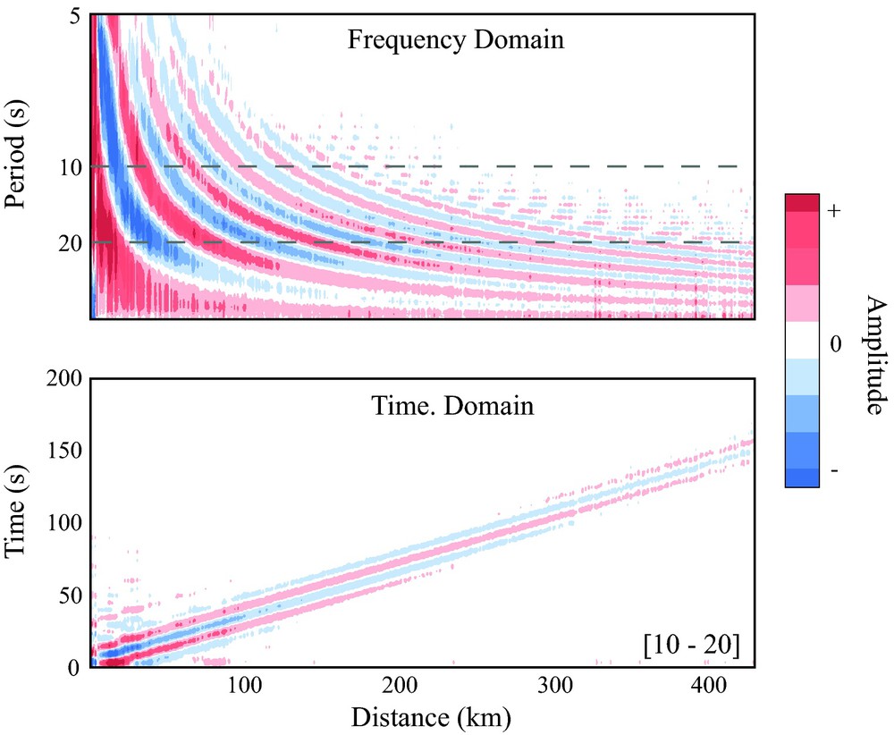
Relationship between spatial (frequency domain) and time domain correlations. Top panel shows frequency domain spatial coherency estimates for southern California data, with characteristic Bessel function shape. Bottom panel is obtained by Fourier transforming the top panel, retrieving the time domain cross-correlation. Time domain is filtered between 10–20 s period, corresponding to the dashed lines on top panel. Equivalent results for phase velocity were obtained.
Relation entre le domaine spectral et temporel (avec la distance) des corrélations. La figure du haut représente les mesures de cohérence en fréquence avec la distance pour les données de Californie du Sud, avec la forme caractéristique de la fonction de Bessel. La figure du bas est obtenue en appliquant une transformée de Fourier de la figure au-dessus, ce qui produit les corrélations en temps. Les séries temporelles sont filtrées entre les périodes 10–20 s, ce qui correspond à la zone entre les lignes en tirets.
Adapted from (Prieto et al., 2009a).
Nevertheless, as discussed above, either method (time or frequency domain) has a limitation in that the power of the ASF is not known a priori. One could try to estimate the values σ or as a function of time, position, or even the direction (Stehly et al., 2006; Taylor et al., 2009; Yang and Ritzwoller, 2008), to obtain a more precise estimate of the Green's function.
A more subtle approach is to try to correct the amplitude of each seismic record (at stations A and B) before performing the cross-correlation. This is sometimes called prewhitening (Bensen et al., 2007) and is the mathematical equivalent (in the frequency domain) of the coherency:
| (5) |
One could alternatively normalize with respect to either of the two stations (following Bendat and Piersol, 2000 in the notation)
| (6) |
| (7) |
Both HAB and HBA are called the transfer function (or frequency response function) of B with respect to A or A with respect to B, depending on the signal used for normalization.
The time domain equivalent of Eqs. (6) and (7) are known as the impulse response function (IRF), denoted in this case with hAB and hBA, respectively. The IRF also has the same phase information (arrival time information) as (4) and (5), but the amplitude information may be different if the ambient field power is not unity or is spatially variable. A more complete discussion of the limitations of the IRF to retrieve the EGF (also known as interferometry by deconvolution) may be found in (Vasconcelos and Snieder, 2008a; Vasconcelos and Snieder, 2008b).
In the following, we will use all three equations (5)–(7) to extract an estimate of the Green's function between seismic stations that record the ASF while keeping not only the phase information (travel time) but also the amplitude information that might be present. The choice of normalization depends on the particular feature of the EGF of interest, as will be explained in each case.
In this study, the amplitude spectrum inside the curly brackets {·} in Eqs. (5)–(7) is estimated for the same time window as the numerator using a multitaper algorithm, not from a daily average amplitude. For the 24-hour or monthly EGF estimates, the normalized estimates are then stacked to the desired time interval. In all cases, the time domain representation of the coherency or of the transfer function is our estimated GF. The coherency is equivalent to performing time-domain cross-correlation after prewhitening each signal individually, while for the transfer functions we obtain the unit impulse response (Bendat and Piersol, 2000).
In short, we use the IRF for the EGF based on the transfer function, and coherency for the EGF obtained through Eq. (5), which is equivalent to cross-correlation after prewhitening, but in the frequency domain.
3 Signal processing
In addition to the need to normalize the records at the different seismic stations to account for the dynamic range of the ASF as a function of frequency (spectral normalization), further processing is often performed. One-bit normalization, threshold clipping or other amplitude normalization (temporal normalization) of the time series is routinely performed before calculating cross-correlations (Campillo, 2006; Sabra et al., 2005; Shapiro et al., 2005). Bensen et al. (2007) discuss the various approaches of temporal normalization.
We explain here our choice of signal processing, which is slightly different from other approaches used in the literature, to be able to retrieve reliable amplitude information. In calculating the ensemble averages for Eqs. (5)–(7) we follow these steps:
- • use short (1-hour) time windows for both numerator and denominator;
- • divide the numerator by the denominator for each 1-hour window;
- • apply no temporal normalization;
- • stack 1-hour estimates to obtain 24-hour, monthly, and yearly averages.
The approach we use reduces uncertainties and the influence of non-stationary signals, such as teleseisms or large regional and local earthquakes, while retaining amplitude information.
3.1 Short time windows
One drawback of using the raw seismic records, that is, not applying temporal normalization (clipping), is that the ASF is non-stationary and is sometimes contaminated by earthquake signals. If an important or high amplitude earthquake is present in the recorded signals, significantly biased results could be obtained.
This is one of the reasons for using amplitude normalization, viz. to reduce the effect of transient signals that contaminate the retrieved EGF. Fig. 2 shows the EGF resulting from using the 24-hour record shown in the top panel. A very strong teleseismic signal is present in the middle of the 24-hour time series. The EGF is calculated in three different ways: (i) apply one-bit clipping and use equation (6) on the complete 24-hour time series; (ii) apply Eq. (6) to the raw 24-hour time series; and (iii) use Eq. (6) on the raw time series, but employ non-overlapping 1-hour windows. Note that for method (iii) the equation is applied for each single 1-hour window and then stacked. The IRF obtained is thus different between methods (ii) and (iii) because of the choice of window length.
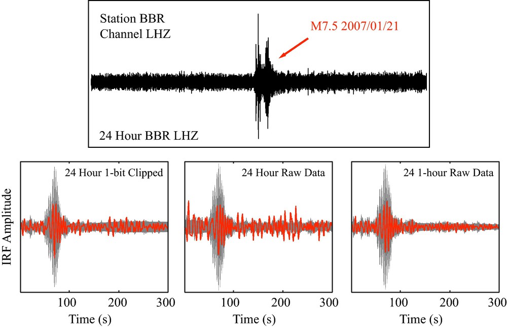
Comparison of processing methods in terms of stability of retrieved EGF between station BBR and LAF. Top panel shows a 24-h record at station BBR. A teleseismic signal is evident in the record and will affect the EGF estimated from this record. Bottom panel shows the EGF (red curve) using the 24-h window above compared to the 2σ amplitude (gray area) of the average EGF using a 5-day stack. First bottom panel shows the standard method used in the literature, viz. 1-bit clipping and EGF calculation using 24-h. Middle panel shows the same method but with the raw data (no clipping), leading to substantial errors in amplitude of the EGF and spurious arrivals. Right panel shows calculation with non-overlapping 1-h windows, stacked. Note that the effect of the ∼ 1-h non-optimal earthquake record is significantly reduced.
Comparaison des méthodes de traitement en termes de stabilité d’EGF récupérées entre les stations BBR et LAF. Le panneau du haut montre un enregistrement de 24 heures à la station BBR. Un signal télésismique est apparent sur l’enregistrement et affectera l’EGF estimée à partir de l’enregistrement. Le panneau du bas montre l’EGF (courbe rouge) utilisant la fenêtre de 24 heures ci-dessus, comparée à l’amplitude 2 s (zone grise) de l’EGF moyenne utilisant une sommation sur cinq jours. Le premier panneau du bas montre la méthode standard de la littérature, c’est-à-dire normalisation 1-bit et calcul de l’EGF sur 24 heures. Le panneau du milieu montre la même méthode mais avec les données brutes (aucun écrêtage), ce qui conduit à de substantielles erreurs dans l’amplitude de l’EGF et à des évènements parasites. Le panneau de droite montre un calcul avec des fenêtres d’une heure ne se recouvrant pas, sommées. On notera que l’effet de l’enregistrement du tremblement de terre, non optimal sur environ une heure est réduit de manière significative.
Method (ii) clearly shows a poorly resolved EGF due to the pervasive effect of the high amplitude teleseismic signal. One-bit clipping significantly reduces its effect, but at a cost of suppressing the amplitude retrieval of the IRF. If, however, we use the raw time series on shorter time windows it seems to work just as well. No spurious arrivals are observed and the 1-day EGF lies within the amplitude of a longer time averaged EGF (gray area). This is true even though the teleseismic signal is used in the 24-hour stack. Its effect is reduced by a factor of ∼24.
3.2 Wave amplification and temporal normalization
In the following, we show how using temporal normalization (one-bit) in ASF processing suppresses basin amplification information. Fig. 3 describes how the use of the IRF can be used to explore the amplification effect of sedimentary basins. After calculating the IRF with respect to the left hand side station (station V) using the ASF, the basin, due to the focusing effects of lower seismic velocities, amplifies the seismic waves.
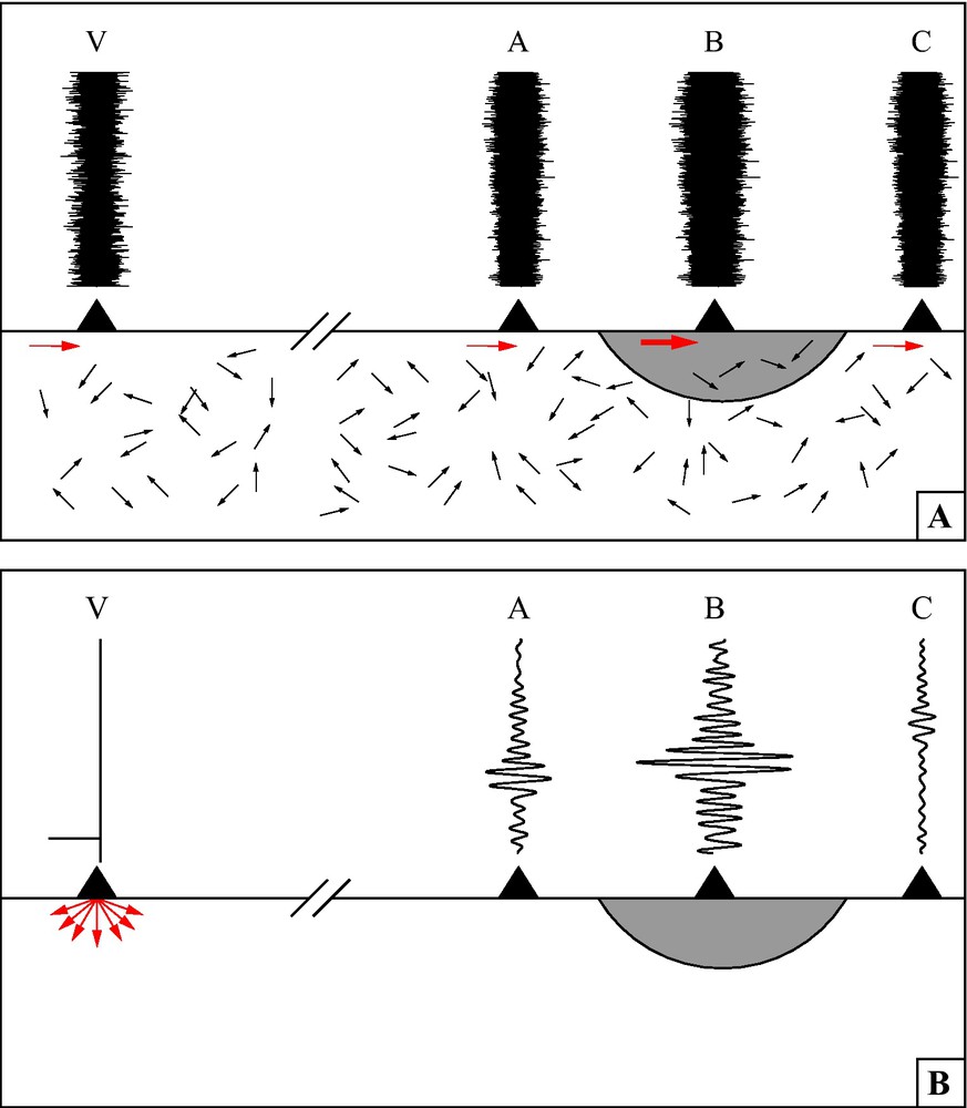
Ambient seismic field and impulse response after deconvolution with a virtual source. (A) Apparently incoherent ambient field records at seismic stations are registered due to distant sources and/or multiple scattering (after Weaver, 2005). Some rays (red arrows) are registered by multiple stations rendering a weakly coherent signal. (B) The IRF with respect to a virtual source (Station V) highlights the coherent signal between the various stations while keeping the basin amplification effect due to a low velocity basin represented by the gray area. Note that with a normalized cross-correlation amplitude information might be obscured.
Champ sismique ambiant et réponse impulsionnelle après déconvolution avec une source virtuelle. (A) Enregistrements du champ ambiant apparemment incohérents, dus à des sources distantes et/ou à leur grande dispersion (d’après Weaver, 2005). Certains rais (flèches rouges) sont enregistrés par de multiples stations, ce qui génère un signal peu cohérent. (B) L’IRF, eu égard à une source virtuelle (station V), met en évidence le signal cohérent entre les stations variées, en conservant l’effet d’amplification du bassin à faible vitesse, représenté par la zone grise. On notera qu’avec une corrélation calculée à partir de bruit normalisé, l’information sur l’amplitude pourrait être perdue.
If the ASF records were clipped before computing the IRF the coherent signal amplitudes would be clipped as well, no amplification effect would be measurable. Note that using the coherency has a similar effect because the cross-correlation is normalized by both the virtual station (station V) and the basin station (station B), thus suppressing the amplification effect.
Fig. 4 shows the EGF obtained from the IRF between seismic station BBR and two stations near Los Angeles (LAF and RPV). The three-components of motion are shown with the EGF between BBR-LAF compared to BBR-RPV. If no temporal normalization is performed the IRF for station LAF always shows higher amplitudes, while if one-bit clipping is applied, the amplitude is similar for both stations. As shown by (Prieto and Beroza, 2008) and later in Section 5, comparing these EGFs with actual earthquake signals, confirms that basin stations like LAF will have higher amplitudes, while station RPV, located in the Palos Verdes hills, on the far side of the basin, will show reduced amplitudes. This difference is also confirmed using numerical simulations of wave propagation across the basin (Komatitisch et al., 2004; Olsen et al., 2006).
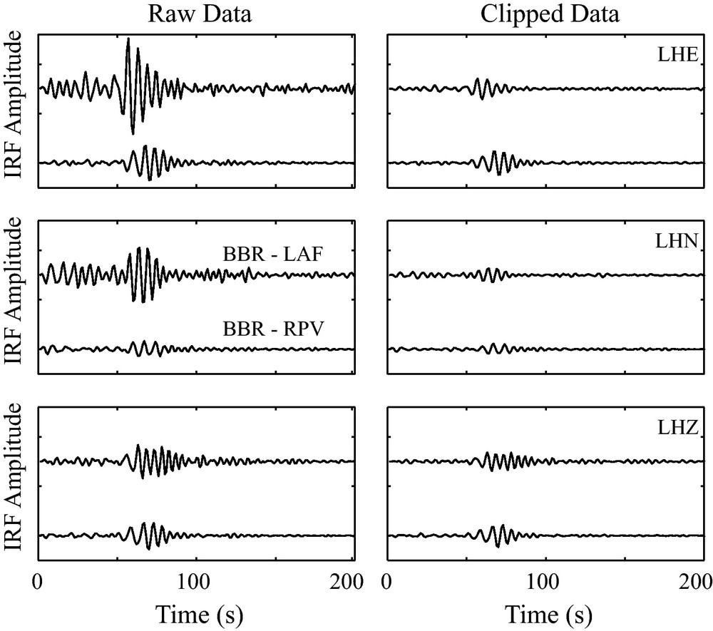
Comparison of processing method using one-bit clipping and unclipped data for the EGF between station BBR (Channel LHZ) and three components of stations LAF and RPV. The waveforms are very similar, but processing with the unclipped data allows the relative amplitude information to be retrieved. Amplitudes at station LAF located inside the LA Basin are always higher than station RPV located in the Palos Verdes hills, west of the Basin. These lower amplitudes on the far side of the basin are also observed in the equivalent numerical simulations.
Comparaison des méthodes de traitement utilisant le codage sur 1 bit et les données non écrêtées pour l’EGF, entre la station BBR (canal LHZ) et trois composantes des stations LAF et RPV. Les formes des ondes sont très similaires, mais le traitement avec les données non écrêtées permet de récupérer l’information sur l’amplitude relative. Les amplitudes à la station LAF située dans le bassin de Los Angeles sont toujours plus élevées qu’à la station RPV située sur les collines de Palos Verdes à l’ouest du bassin. Ces amplitudes plus faibles sur cette partie éloignée du bassin sont aussi observées dans les simulations numériques.
Komatitisch et al., 2004; Olsen et al., 2006.
3.3 Attenuation information and temporal normalization
Some authors have reported retrieving amplitude information from noise EGF (Larose et al., 2007; Weaver and Lobkis, 2001). Larose et al., 2007 discussed this issue using laboratory experiments and concluded that both prewhitening (coherency) and one-bit normalization do not allow recovery of the correct GF decay compared to an active experiment. In contrast, other authors (Cupillard and Capdeville, 2010; Matzel, 2007) have presented evidence that even with one-bit normalization geometrical spreading and attenuation information are retrieved. More recently Cupillard et al. (2011) have confirmed that the one-bit correlations still contain this kind of information in their numerical experiments.
This counter-intuitive observation can be explained because the Earth's structure reduces the coherent signal as a function of distance due to geometrical spreading, attenuation and scattering. The cross-correlation coefficient between increasingly distant stations is thus likely to be reduced and the amplitude of the EGF will decrease with distance. The coherency describes the signal-to-noise ratio between coherent and incoherent noise (red rays versus black rays in Fig. 3). From a theoretical point of view and a numerical perspective, Cupillard and Capdeville (2010) and Cupillard et al. (2011) demonstrated that geometrical spreading and attenuation were retrieved even for clipped data if appropriately distributed sources are available.
From the previous subsections, it is clear that if we want to study basin amplification we need to use the IRF (coherency not useful) and not apply temporal normalization. If we are interested in distance-dependent amplitudes (geometrical spreading and attenuation) we can use the coherency (Eq. (5)) and optionally the one-bit normalization. In this study for simplicity, we decided not to apply any type of temporal normalization, other than using small windows for calculating the IRF and the coherency.
4 Engineering applications of the IRF
The impulse response function has been used in the past for a variety of applications. The IRF is basically the deconvolution of two seismic records, which is similar to the method of earthquake receiver functions (Helffrich, 2006; Schuster et al., 2004). This kind of deconvolution is used to study the near-surface effect by deconvolving the records at various depths with respect to a deeper seismic station located in a borehole. Not only travel times, but also attenuation may be estimated for the shallow structure (Abercrombie, 1997; Mehta et al., 2007). This deconvolution is in many cases performed in order to remove the source excitation from the records.
Snieder and Safak (2006) used the IRF calculated from earthquake data to extract the building response of the Millikan Library. They deconvolved the recorded motions due to an earthquake at the various floors with respect to the bottom floor sensor to estimate the shear wave velocity and attenuation of the building. A similar earthquake-based approach was also presented for the Factor Building in UCLA (Kohler et al., 2007).
Prieto et al. (2010) show that ambient vibrations of the building can also be used to calculate the IRF. Here we use data from the Factor Building, a 17-story, steel, moment-frame building at the University of California, Los Angeles, instrumented with a 72-channel array of accelerometers in a unique structural state-of-health monitoring experiment (Kohler et al., 2005).
We calculate the IRF for the Factor Building by deconvolving the records at all of the building floors with respect to the records at one of the floors (bottom floor, eighth story and the top floor). We perform this deconvolution via a multitaper algorithm (Prieto et al., 2009b) over a time span of 50 days. Fig. 5 shows the motion of the Factor building after deconvolution with the motions at the top floor, the 8th story and the bottom floor, filtered between 0.5–5.0 Hz. Note that for each IRF panel, the signal at the source station is a filtered delta function. The velocity of the upgoing and downgoing waves can be measured as well as the attenuation of the waves as they propagate up and down the structure (Prieto et al., 2010).
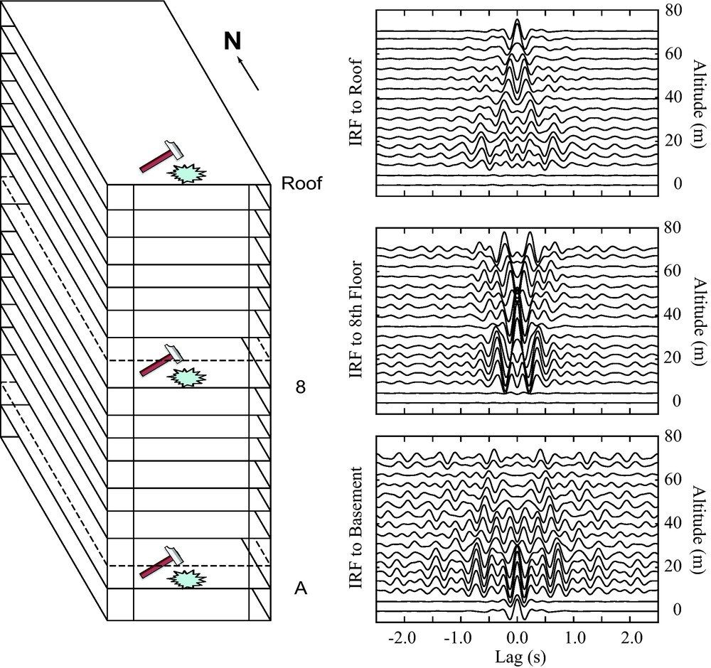
Impulse response functions for the Factor building as determined by applying a virtual source at different floors of the structure. Note that this IRF is not equivalent to the Green's function because of different boundary conditions imposed.
Fonctions de réponse impulsionnelle pour le bâtiment Factor, par application d’une source virtuelle aux différents étages de la construction. On notera que l’IRF n’est pas équivalente à la fonction de Green en raison des différentes conditions aux limites imposées.
Snieder, 2009.
It is important to understand that the result of the IRF is not exactly the GF of the building. Even though the phase information is the same, the IRF is subject to a different boundary condition (Snieder, 2009; Snieder and Safak, 2006). The virtual source is a unit impulse at time τ = 0 and zero otherwise. For example, in Fig. 5, the IRF shows no shaking on the 8th floor at large lag times due to the boundary conditions imposed.
Fig. 6 shows the IRF with respect to the bottom floor filtered on three different frequency bands (0.4–0.6, 1.4–2.0 and 2.5–3.5 Hz) close to first three modes of the Factor building. The waveforms at different floors clearly show the amplitude of shaking for the three different modes and the nodes of the second and third modes. It can also be seen that the amplitude of shaking of the different modes decreases with increasing time, which can be related to attenuation in the building. Kohler et al. (2007) using earthquake data and Prieto et al. (2010) using ambient vibrations have successfully estimated the attenuation of the Factor building for the different modes by fitting of a line to the log of the envelope function of the filtered time series and relating Q to the slope of the line.
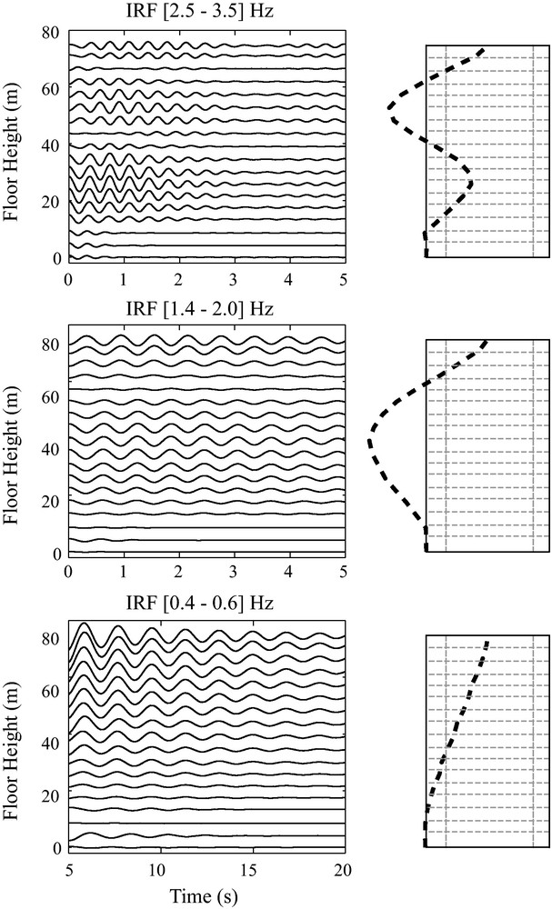
IRF amplitudes and modes of vibration of the Factor Building. Left panels show the IRF with respect to the bottom floor (bottom panel in Fig. 5) filtered at various frequency bands near the modes of the Factor Building (Kohler et al., 2005). Right panels show the mode shapes determined from the narrowband IRF. The signals were normalized to the same maximum value for each mode. Note that amplitude of shaking varies as a function of frequency and height, depending on the modes of vibration. Amplitude information is fundamental to correctly describe building response. The building outline is shown for reference.
Amplitudes de l’IRF et modes de vibration du bâtiment Factor. Les panneaux de gauche montrent l’IRF par rapport à la base (panneau du bas de la Fig. 5), filtrée à des bandes de fréquence variées, proches des modes du bâtiment (Kohler et al., 2005). Les panneaux de droite montrent les modes déterminés à partir de l’IRF filtrée de gauche. Les signaux sont normalisés à la même valeur maximum, pour chacun des modes. On notera que l’amplitude des vibrations varie en fonction de la fréquence et de la hauteur, dépendant des modes de vibration. Le schéma du bâtiment est présenté comme référence.
5 Basin amplification in EGF based on IRF
A source of particular concern for seismic hazard analysis is the effect of large sedimentary basins on earthquake strong ground motion. Basin amplification is a major problem for many large urban centers in the world (Los Angeles, USA; Tokyo, Japan; Mexico City, Mexico; and Bogota, Colombia to cite just a few) because basins trap and amplify seismic energy (Komatitisch et al., 2004; Olsen et al., 2006; Stidham et al., 1999; Vidale and Helmberger, 1988) and thus increase vulnerability to earthquakes.
5.1 Amplitude comparison with earthquake records
Previous authors have compared earthquake records with EGF (Shapiro et al., 2005) and have proposed to use these EGF for improving earthquake locations (Barmin et al., 2011). Prieto and Beroza (2008) showed that it is possible to extract reliable phase and amplitude response from the ASF Green's functions using the IRF. They presented a comparison of the complex ground motions associated with a moderate earthquake in California and the IRF showing strong similarity in waveform shape and amplitudes.
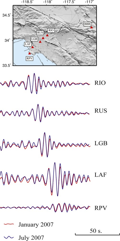
Here, we present another example in Fig. 7. The concept is similar to that applied for building response. In the long-period range [4–10 s period], it is possible to document basin amplification from the EGF obtained via IRF. Since the main source of ASF in southern California is located to the west (Stehly et al., 2006; Yang and Ritzwoller, 2008) for this frequency band, we use the station closest to the coast to normalize the deconvolution. Amplitude measurements are more reliable for stations pairs aligned perpendicular to the dominant source region (the coast). Fig. 7 shows the radial component waveforms from a M5.1 earthquake near station HEC in southern California with IRF at stations in the Los Angeles Basin (LAB) showing very similar features. The observed basin amplification of the earthquake records is also observed in the IRF for a virtual source located at HEC at periods between 4–10 s.
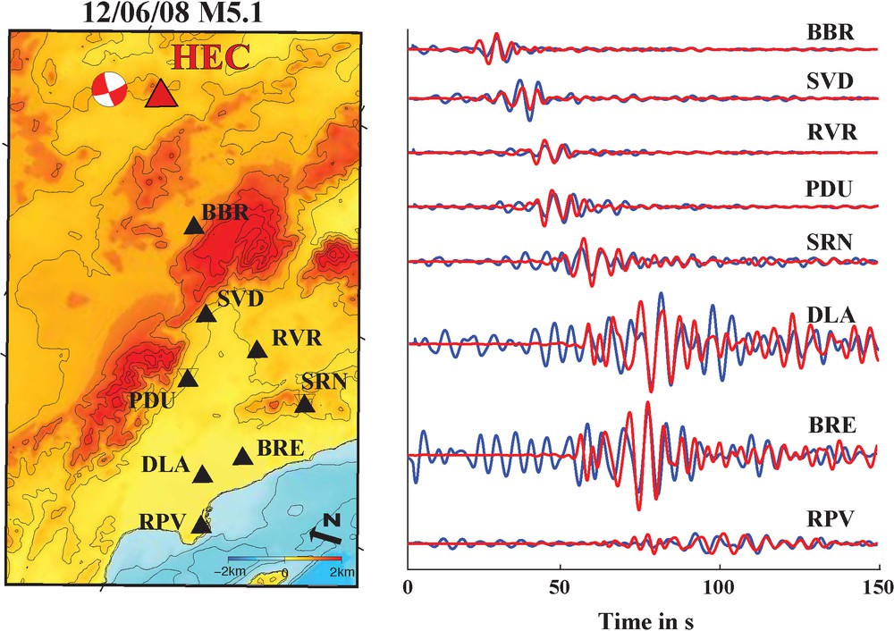
Comparison of recorded waveforms of the M5.1 earthquake on 12/06/2008 (red) and EGF obtained from the IRF with respect to station HEC (blue). Left panel shows a location map of the seismic stations used. Right panel shows waveforms filtered between [4–10] s period. Basin amplification observed in the earthquake records is also observed with IRF.
Comparaison des formes d’onde du tremblement de terre M5-1 enregistrées le 12/06/2008 (en rouge) et EGF obtenu à partir de l’IRF à la station HEC (en bleu). Le panneau de gauche présente la carte de localisation des stations sismiques étudiées. Le panneau de droite montre les formes d’ondes filtrées pour des périodes de [4–10] s. L’amplification induite par le bassin et montrée par les enregistrements du tremblement de terre est aussi observée avec l’IRF.
5.2 Stability of Amplitude retrieval
Meier et al. (2010) show that small seasonal variations of the velocity (<0.1%) in the LAB can be observed in the three years of observations they made and suggest that they are not due to the source of the ASF. Our amplitude measurements may complement this kind of seasonal variation studies in sedimentary basins. Fig. 8 shows basin amplification for two virtual sources located to the east of the Lab. The contour plots show the peak displacement amplitude of the IRF after a geometrical correction factor proportional to the square root of the propagation distance is applied. Results represent two different months illustrating the stability of the amplitude retrieval. The similarity of the amplification maps shown in Fig. 8 suggests that the amplification effect observed is a strong and reliable feature. We cannot conclude based on these results that the small variations observed between the two time ranges are due to small changes in the velocity or attenuation structure or they are due to temporal variations of the ASF; a longer time span similar to that of Meier et al. (2010) is needed.
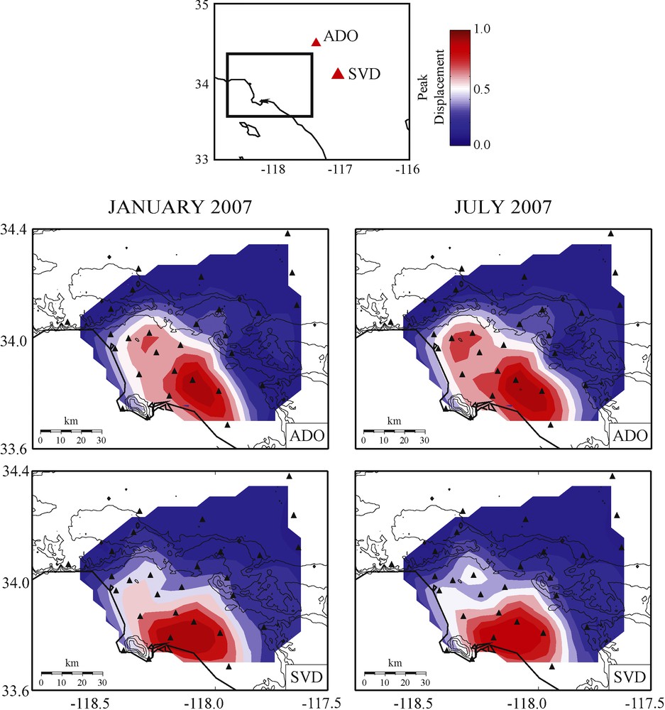
Predicted amplitude response of Los Angeles Basin stations to virtual sources at two different stations (ADO and SVD) close to the San Andreas Fault. A geometrical spreading correction factor was applied to isolate the basin amplification effects. Results from two distinct months (summer and winter months) are similar.
Amplitude prédite par la réponse du bassin de Los Angeles à deux sources virtuelles localisées près de la faille de San Andreas, aux stations sismiques ADO et SVD. Un facteur de correction d’expansion géométrique a été appliqué, de manière à isoler les effets d’amplification du bassin. Les résultats obtenus pour deux mois distincts (mois d’été et mois d’hiver) sont similaires.
As discussed above, the relative amplitude information retrieved using the IRF shows stability comparable to observed earthquake records. Fig. 9 shows a subset of the waveforms used to generate Fig. 8. A comparison of the amplitude as well as the waveforms shows remarkable similarity, again confirming that the result is not significantly affected by the month of the year or the location and strength of the ASF.
Impulse response functions between station BBR and selected Los Angeles Basin stations. Data from two distinct months (summer and winter months) are processed showing very small variations of the amplitude information. A total of 100 s of the IRF is shown. Top panel shows locations of the seismic stations.
Fonctions de réponse impulsionnelle entre la station BBR et des stations sélectionnées dans le bassin de Los Angeles. Le traitement des données acquises lors de deux mois distincts (un mois d’été et un mois d’hiver) montre de très faibles variations de l’information sur l’amplitude. Un total de 100 s de l’IRF est présenté. Le panneau du haut montre la localisation des stations sismiques.
The waveforms shown in Fig. 9 were generated with a month-long data series and suggest that, at least for the frequency range considered here ([4–10] s period), amplitude information is stable and reliable (comparable with observed earthquake records). We expect that for higher frequencies of interest for engineering application (see previous section for example) EGF retrieval at such distances will be difficult and may be less stable. Much longer time intervals may be required to retrieve amplitude information with the same level of confidence or stability.
6 Attenuation
The previous sections show the importance of the EGF for amplification variations studies. The first experiments of Weaver and Lobkis (2001) showed that both the phase and amplitude of the signals were passively reconstructed. From the previous sections and various published results (Matzel, 2007; Prieto and Beroza, 2008; Prieto et al., 2009a; Taylor et al., 2009), it can be deduced that the amplitude information carried in the EGF may help in studying aspects of the wavefield beyond travel time.
A 1D model of the depth-dependent Q-structure in southern California (Prieto et al., 2009a) was obtained via ASF analysis, yielding results consistent with other independent studies of earthquake records (Yang and Forsyth, 2008). Furthermore, lateral variations in attenuation between two distinct regions (large sedimentary basins in southern California vs the rest) were clearly observed using a regionalization approach.
Cupillard and Capdeville (2010) generated synthetic seismic noise on the surface of a spherical attenuating Earth and computed cross-correlations of records from stations along a linear array. One-bit, raw, and prewhitening processing were performed. They found that if sources are evenly distributed, both attenuation and geometrical spreading were recovered even after temporal or spectral normalization. This was recently confirmed in Cupillard et al. (2011), where the distance dependent geometrical spreading and anelastic attenuation are preserved in one-bit correlations.
These observations suggest the possibility of performing attenuation tomography using the ASF. Here we extended the methods presented in Prieto et al. (2009a) to perform 2D tomography of the western United States using the ASF.
6.1 Method for attenuation tomography
As discussed above, the real part of the coherency of the ASF at two distinct stations has the shape of a Bessel function J0
| (8) |
The previous relationship holds only for elastic (non-scattering) media, however, an additional exponential decay must be added to properly describe an attenuative or scattering medium (Larose et al., 2007; Mitchell, 1995; Romanowicz, 2002). Note that the method proposed here does not allow for anelastic and elastic scattering effects to be separated, since the elastic scattering also adds an exponential decay, depending on the correlation length of the medium (Aki and Chouet, 1975; Anache-Ménier et al., 2009).
For an attenuating medium, an appropriate parameterization for the coherency is then
| (9) |
The method presented by (Prieto et al., 2009a) uses Eq. (9) to find the velocity and attenuation for a large array of seismic stations after azimuthal averaging of coherencies at similar offsets and fitting the equation for multiple distances. As proposed in Cupillard and Capdeville (2010), the attenuation effect is present in the noise correlations if a uniform distribution of noise sources is available. Azimuthal averaging is useful to reduce the effect of a non-uniform noise distribution.
We adopt the method of Prieto et al. (2009a) in order to examine the lateral variation of attenuation and velocity structure. We regionalize the seismic network using overlapping sub-arrays and apply Eq. (9) to find the optimal phase velocity and attenuation coefficient for each array.
We parameterize the western US with 6400 (0.25° × 0.25°) grid cells and calculate spatial coherencies at 8-s period at stations surrounding each cell. Note that the estimated values of phase velocity (C(f)) and attenuation coefficient (α(f)) for each grid cell represent an average over a broad area. The resulting data at each grid cell is then inverted for a 2D map using LSQR (Lawson and Hanson, 1974; Paige and Saunders, 1982).
6.2 Tomography results
Fig. 10 shows the phase velocity and attenuation coefficient maps (Lawrence and Prieto, 2011) obtained by analyzing ASF for a 2-year time interval. The 8-s period attenuation map shows very strong attenuation for the Pacific Northwest, Yellowstone, along the west coast and high attenuation in California's Central Valley as previously reported using other methods (Clawson et al., 1989; Hwang and Mitchell, 1987; Lawrence et al., 2006; Phillips and Stead, 2008).
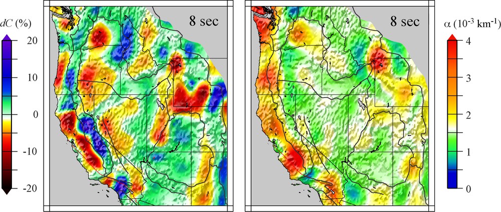
Tomographic maps of phase velocity perturbation and attenuation coefficients across the western United States in the 8-s period range. The methodology to obtain these maps is briefly explained in the text (Section 6.1) and in (Lawrence and Prieto, 2011). Velocity perturbation with respect to a constant velocity model.
Cartes tomographiques de perturbation de la vitesse de phase et des coefficients d’atténuation à travers l’Ouest des États-Unis dans une gamme de périodes autour de huit secondes. La méthodologie pour l’obtention de ces cartes est brièvement expliquée dans le texte (Section 6.1) et dans Lawrence et Prieto (2011). Les perturbations de vitesse sont représentées par rapport à une vitesse moyenne.
Strongly attenuating features (Fig. 10) seem to be correlated with low seismic velocities under large sedimentary basins, such as California's Central Valley, the Oregon-Willamette Valley and the Puget Sound Basin along the west coast (Hwang and Mitchell, 1987; Pratt and Brocher, 2006). Strong attenuation (low Q) is also evident under Yellowstone and may be attributable to high temperatures and/or partial melt in the crust related to hot-spot vulcanism (Fan and Lay, 2003; Xie, 2002).
It has long been known that 3D velocity structure may (de)focus seismic energy along velocity heterogeneities, leading to amplitude anomalies due to elastic effects that could be mis-modeled as the signature of attenuation (Dalton and Ekström, 2006; Lay and Kanamori, 1985; Selby and Woodhouse, 2000; Tian et al., 2009; Woodhouse and Wong, 1986). If our measurements were systematically biased by focusing, we would expect predominantly high attenuation anomalies in high velocity regions and vice versa in Fig. 10. Similarly, while source heterogeneity may contaminate the observed attenuation structure to some degree (as suggested by Harmon et al., 2010), this effect is likely small, since attenuation features are more strongly correlated with tectonic features than they are with station distribution or proximity to the coast.
6.3 Stability of attenuation estimates
It has been suggested that even though an EGF may be obtained from correlations of ASF data, attenuation or other results involving more accurate amplitude information may be biased due to varying sources in the ASF, directivity of the ASF, or simply because some of the conditions required in theory for GF retrieval may have to be more strictly followed if amplitude information is studied (Cupillard et al., 2011; Harmon et al., 2010; Snieder et al., 2009).
Figure 11 shows estimated attenuation coefficients for distinct time intervals. Results for the different time periods show remarkable similarity and suggest that, if present, the bias due to the distribution of ASF noise is not large. Many authors have studied seasonal variation of the ASF (Gerstoft and Tanimoto, 2007; Stehly et al., 2006; Yang and Ritzwoller, 2008 and others). For example, in the frequency band between [10–20] s the azimuth of the ASF energy changes significantly during summer and winter months while our 3-month attenuation coefficients vary by less than 10% over the 12-month period studied (Fig. 11).
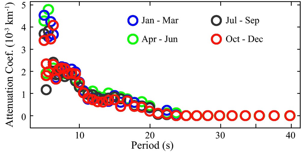
Stability of attenuation coefficient estimates. Estimated attenuation coefficients for data subsets in southern California for various non-overlapping 3-month periods. Estimates are made following (Prieto et al., 2009a). Larger uncertainties are present at higher frequencies, but in general the plot suggests little temporal variations of the attenuation coefficient estimates.
Stabilité des estimations du coefficient d’atténuation. Coefficients d’atténuation estimés pour des sous-ensembles de données obtenues dans le Sud de la Californie, sur des périodes de trois mois ne se recouvrant pas. Les estimations sont effectuées suivant (Prieto et al., 2009a). De plus grandes incertitudes apparaissent pour les hautes fréquences, mais en général, le graphique suggère peu de variations temporelles dans les estimations de coefficient d’atténuation.
Harmon et al. (2010) show results of their own with strongly varying attenuation estimates and uncertainties that are of the same order as the expected attenuation coefficients, which is in conflict with what is shown in Fig. 11. A possible source of this discrepancy comes from the signal processing methods used in the two studies. As discussed above (Section 3), in order to retrieve reliable amplitude information, we eschew amplitude clipping and opt to use many windows of shorter duration for our coherency estimates, while Harmon et al. (2010) use 24-hour long series with envelope normalization. As shown in Fig. 2 using 24-hour windows may introduce strong amplitude variations from teleseismic, local, or regional earthquakes.
It is clear that further study of the ASF source location and amplitude characteristics is required for more accurate attenuation coefficient estimates. So far, in order to reduce the effect of the direction of the ASF, we apply azimuthal averaging as suggested by Prieto et al. (2009a). Tsai (2009) showed that, ideally, we should weight the contributions to the GF by the square-root of the source amplitude and inversely with the duration of source prevalence in order to retrieve a better estimate of the EGF. One approach is to use f–k analysis or other array methods (Bromirski and Gerstoft, 2009; Gibbons et al., 2009; Schulte-Pelkum et al., 2004; Zhang et al., 2009) to discern the direction of the ASF and its amplitude, but this is itself not free of uncertainties and is well beyond the scope of this article.
7 Discussion and conclusions
In this article, we present evidence that useful amplitude information is present in ASF Green's functions, and can be used to understand the response of engineered structures, to map amplification effects due to sedimentary basins, and as the basis for attenuation tomography. Two main estimators based on the ASF were used, depending on the amplitude feature of interest.
The spectral coherency is a measure of signal to noise ratio between coherent and incoherent signals. The decrease of coherency with increasing station separation is then related to both geometrical spreading and attenuation. Because of the spectral normalization in the coherence estimate, any amplification or local site effect will be removed.
In contrast, the IRF can be used to describe basin amplification and we showed that similar amplitude effects are observed from local earthquakes in California. In the particular case of an engineered building, the IRF shows how the shaking varies both as a function of floor height and frequency (modes). Although not shown here, mode attenuation information can also be estimated from the IRF (Prieto et al., 2010).
As shown in the early examples (Section 3) the approach to signal processing can make a big difference in the quality of the results:
- 1. temporal normalization, although important to reduce the effect of non-stationarity and earthquake signals, may interfere with the ability to retrieve some types of amplitude information;
- 2. we suggest using shorter time windows without temporal normalization. Amplitude information is maintained and the deleterious effects of earthquakes or other non-stationary noise sources are reduced. This approach comes with limitations, including reduced frequency resolution and shorter EGF length retrieved. A criteria for not using certain windows (with strong signals) can also be added (Prieto and Beroza, 2008; Prieto et al., 2009a);
- 3. in theory, the correlation of a diffuse field yields the GF, but in practical applications some type of temporal or spectral normalization is usually required. Since, in most cases, we don’t know the nature and power of the sources, we use the recorded signals for normalization. We present here two cases: EGF based on the IRF, and EGF based on the coherency and their applications for amplitude retrieval.
The conditions that in theory need to be satisfied for GF retrieval are not satisfied in realistic conditions; yet, there is clear evidence that useful results are recovered from the ambient seismic field. It may be that scattering helps to realize a correct GF retrieval (Campillo and Paul, 2003; Derode et al., 2003; Gouédard et al., 2008; Stehly et al., 2008), but for attenuating media, the conditions are more strict (volume sources, see Snieder et al., 2009 and references therein). Thus, the results for basin amplification and attenuation from the ASF are more likely to be biased. We present, for both measurements of amplification and attenuation, evidence that this bias is not substantial, and find results that are consistent with those determined using earthquake records. Similar encouraging results from numerical experiments have been presented (Cupillard and Capdeville, 2010).
We believe the amplitudes available in the EGF provide additional and complementary information from that of EGF travel times. Attenuation, for example, is critical for discriminating between temperature or volatile content variations within the Earth, and complements information extracted from wave speeds (Karato, 1993, 2003; Priestley and McKenzie, 2006). In large sedimentary basins lower wave speeds tend to amplify seismic waves, but because of fluid content and scattering in these regions, attenuation is also important and needs to be accounted for to enable accurate ground motion simulations (Komatitisch et al., 2004; Olsen et al., 2006; Power et al., 2008).
The ASF Green's functions show remarkable similarity to ground motions recorded for earthquakes, both in phase and amplitude (Prieto and Beroza, 2008). Propagation and amplification effects between an earthquake source region and a large urban center can be tested using the ASF by placing seismic stations along active faults. These long-period ground motions are most relevant for structures that are sensitive to long-period ground motions, i.e., for very tall buildings or long-period bridges. A direct prediction of ground motion amplitudes recorded at a remote, tall building would represent a source-to-rafter prediction without the effort of modeling the complex geology and soil-structure interaction.
There remain issues to be addressed if EGF ground motion predictions are to be used. Earthquake radiation patterns are different than a simple source EGF and depth dependence of the wave excitation needs to be accounted for. For attenuation tomography, the resolution of the models are lower than those of wave-speeds due to the need for regionalization. Future work will try to address and overcome that restriction.
There is great potential, as shown in this special issue, of ASF derived EGF in studying the interior of the Earth. It may be possible to use the amplitude information for time-dependent seismic monitoring using the ASF. So far, only the phase has been used (Brenguier et al., 2008a; Brenguier et al., 2008b), but attenuation variations may have similar, or possibly even stronger effects, if changes to crustal fluids are involved.