

1 Introduction
Reactive transport modelling in porous media is a powerful tool for studying water-rock interactions; it is used to improve the understanding of groundwater pollution, underground waste and carbon dioxide storage, metallogenesis, the environmental impact of mining plants, etc. In the last two decades, great efforts have been made to enhance the capabilities of modelling tools to keep pace with the problems that they can successfully handle (unsaturated media, multiphase flow, non-isothermal flow, redox reactions, complex kinetics, microbiological activity, etc). Surprisingly, an important facet of reactive transport modelling has often been disregarded: description of the intrinsic spatial variability of geological media that is present at every scale. The main reasons is a lack of real geochemical data needed to evaluate the spatial variability of the geological formations at the relevant scale (i.e. between the REV, Representative Elementary Volume, and the size of the simulation domain), and the insufficient CPU-power needed to run the models, which limits the spatial discretizations to a few thousand grid nodes to keep the runtimes acceptable. Very recently, mainly due to increasing CPU capacity and a growing concern about the heterogeneity of the geological medium, an increasing number of authors tend to set initial conditions including spatial variability on some parameters in their simulations (Gödeke et al., 2008; Hammond et al., 2011; Li et al., 2010; Malmström et al., 2008). However, the effects of this variability have not been systematically studied so far.
The purpose of this study is to examine and quantify the impact of spatial variability on the results of 2D reactive transport simulations, with a particular focus on the role of chemistry feedback on hydrodynamics, which is triggered by the dissolution of primary minerals resulting in increased porosity and, possibly, permeability. A simple chemistry and a very simple geometry were chosen in order to properly handle the impact of the initial spatial variability as well as that of the kinetic and hydrodynamic flow conditions on the results of the numerical experiments.
In this study, permeability and porosity fields with spatial variability are considered. Variable mineral concentrations were also investigated, but will be discussed only briefly. Non-conditional geostatistical simulations of permeability and porosity were performed, covering a range of values for the most relevant parameters (see discussion in Section 3.1), in order to establish a hierarchy among them.
The article is organized as follows: first a brief overview of the relevant concepts and methods of geostatistics and reactive transport modelling, the spatial models and the chemical system chosen for this study are discussed; then the results for homogeneous media are shown, to clarify the representation of the system and give a reference for the heterogeneous media simulations. The observable quantities chosen to represent the results are explained and discussed; finally, we discuss the results of numerical experiments, pointing out the effects of each parameter.
2 The tools
2.1 Spatial models and geostatistical simulations
Geostatistics is a well established branch of statistics and probability theory dealing with spatial processes, i.e. with variables defined over a spatial domain and referred to a specific volume, called support. It was theoretically founded by G. Matheron in the 1960’s, and found its main application in mining and oil exploration. It is currently applied to virtually every discipline of the geosciences. A thorough and insightful overview of the theory is given in Chilès and Delfiner (1999), to which the reader can refer to for more details. The fundamental notion of geostatistics is the spatial autocorrelation function; more generally, the semivariogram, or just variogram, depicts the spatial variability of the process Z between two distinct points of the domain, as a function only of their distance:
| (1) |
The assumption of second-order stationarity1 and ergodicity is sufficient to establish the existence of a variogram function, which is non-negative and usually monotonic, and which can be modelled by means of simple analytic expressions. Throughout this study, a unique variogram model is used, the isotropic spherical model, which is a truncated polynomial function:
| (2) |
For multivariate problems, the cross-variogram between variables Z1 and Z2 represents the correlation between their increments:
| (3) |
To address and model the correlation between porosity and permeability, the intrinsic model of co-regionalization was chosen: all direct- and cross-variograms are multiples of a base model (Chilès and Delfiner, 1999). This is achieved by the following construction for the simulation of permeability (noted as k) and porosity (ω):
| (4) |
The joint spatial distributions of permeability and porosity are obtained by non-conditional geostatistical simulations on fine, regular grids by the Discrete Fourier Transform algorithm (Pardo-Igúzquiza and Dowd, 2003). This technique was chosen for its speed and for the immediate possibility of obtaining a family of Gaussian fields with different correlation lengths from a single set of random numbers. This feature allows the direct comparison of results obtained from geostatistical simulations with different correlation lengths (or other parameters), effectively filtering the effect of the additional variability that would have been obtained from several realisations.
The Gaussian random variables are then transformed into log-normal fields to match the classical distribution used for permeability:
| (5) |
| (6) |
| (7) |
To summarize, when the variogram model and the averages of porosity and permeability are fixed once and for all, the multivariate spatial model is completely defined by three parameters: the correlation length a of the variograms, the standard deviation σlogK of permeability and the correlation coefficient ρ between log K and log ω.
2.2 Reactive transport code
Reactive transport simulations were made with the coupled program HYTEC, developed at the MINES ParisTech (van der Lee et al., 2003). In HYTEC, the hydrodynamic part (flow, multicomponent transport, heat transport) is solved by a finite-volumes approach on unstructured grids based on Voronoï polygons. Reactive chemistry is evaluated by chess, also developed at MINES ParisTech (van der Lee, 1998). It determines aqueous speciation, ionic exchange, surface complexation, mineral precipitation and dissolution, assuming either local equilibrium, or a dynamic mixed status of equilibrium/kinetics.
An upscaling method for permeability is necessary to link the fine-gridded geostatistical simulations and the coarse, non-regular grids used in the coupled transport-chemistry modelling (Renard and de Marsily, 1997). Such techniques were introduced and thoroughly discussed in De Lucia (2008, 2009): they were defined in the most general case of unstructured discretizations used by HYTEC, and are based on the properties of Voronoï polygons (same surface of triangles on both sides of the boundary between elements) and of the finite volumes scheme (the calculation is restricted to the component of flow orthogonal to the boundary between elements). The reader is referred to De Lucia et al. (2009) for further details.
2.3 Hydrochemical setting
The investigated chemical system depicts the dissolution of calcite (CaCO3) following the injection of hydrochloric acid HCl. This reaction has several applications, e.g. in the work-over of oil-producing wells. More generally speaking, it can be considered a schematic illustration of an acid attack on carbonate rocks, a process expected to govern, for instance, the natural development of karstic systems, or in geological storage of CO2. From the point of view of chemistry feedback acting on the hydrodynamics, it represents a case of increasing porosity.
The reaction can be written for example:
| (8) |
| (9) |
Under the thermodynamic equilibrium assumption, the mass action law constrains the chemical speciation via the formation constant
| (10) |
| (11) |
Intuitively, primary mineral dissolution modifies the pore structure of the medium, thus triggering a feedback modification of its hydrodynamic properties, affecting flow and transport. The models working at the REV scale are intrinsically not able to take into account such feedback; it is therefore crucial to introduce further information in the model. The simplest way is to relate porosity (an extensive variable, calculable by a mineral volume balance) and permeability by an empirical relationship. To this purpose, the same Bretjinski’s law (Eq. (6)) used to correlate the macroscopic porosity and permeability spatial variability was chosen to change the permeability as a function of porosity changes:
| (12) |
2.4 Transport equations and non-dimensional numbers of Péclet and Damköhler
Considering the macroscopic (Darcy) scale, the governing equations are established without attempting to derive an upscaled equation from mass and momentum conservation equations defined at the microscopic scale.
The advection-dispersion equation for a transported concentration Ci reads:
| (13) |
The right hand side of this equation corresponds to a reaction rate governed by the only mineral (calcite) present in the domain. kh is the kinetic constant adopted in HYTEC (Eq. (11)) and νi the stoichiometric coefficient of the i-th aqueous species in the chemical reaction of calcite dissolution (Eqs. (8) and (9)). All variables are at this point defined over the blocks of the spatial discretization used in the reactive transport code, which is supposed to be sufficiently larger than the Representative Elementary Volume for the investigated porous medium.
In reaction kinetics, competition arises between the amount of hydrodynamically transported reactive substances and that consumed by the reactions. This relationship is summarized by the non-dimensional Damkhöler number (Da). Da is generally defined as the ratio between the characteristic times of kinetics and advection; however, its precise definition is to some extent arbitrary, and has to be adapted to the particular problem and the specific formulation of reaction kinetics adopted (i.e. the kinetic order - see Golfier et al. (2002) and further references therein, (Battersby et al., 2006; Kalia and Balakotaiah, 2007; MacQuarrie and Mayer, 2005; O’Brien et al., 2003). We chose the definition for a domain-scale Damköhler number by Knapp (1989); Lasaga (1998):
| (14) |
The Péclet number Pe is in turn defined as:
| (15) |
| (16) |
In practice it is difficult to separate the contribution of the effective diffusion and that of the kinematic dispersion; therefore in the following we will vary the Péclet number only by adjusting the dispersivity α, and have fixed the effective diffusion coefficient De in the models at a quite small value (1 × 10⁻¹⁰ m2 s−1).
The combined use of Pe and Da, as pointed out in Cohen et al. (2008); Golfier et al. (2002), is a means to classify the behaviour of the system with respect to the dissolution pattern (formation of wormholes, ramified channels or uniform dissolution).
Both non-dimensional groups are time-dependent: the mineral dissolution modifies the porosity, hence the permeability, and finally the velocity field (Luquot and Gouze, 2009). One can also define local Pe and Da, i.e. varying over the discretized domain. Intuitively, a single value only poorly describes the effective regime inside the whole domain; yet this value is good enough to return a predictive measure of the overall behaviour of the system, as will be shown in the following.
3 Set-up of the model
3.1 Overview of the numerical experiments
The studied hydrodynamic system is quite simple: a square permeameter with prescribed Darcy velocity and concentration at the inflow, and at the outflow imposed hydraulic head and zero concentration gradients (i.e. free outlet); the lateral walls are impermeable limits with no-flow conditions. Such a system is clearly of limited interest for practical applications; nevertheless, it has the advantage of greatly simplifying the comprehension of the results: the fluids and the reactants enter the system at a constant rate due to the particular boundary conditions, independently of the permeameter properties and, most importantly, of its subsequent evolution with the reactions.
It is a definite choice to describe the system non-dimensionally. In fact, the presented results are independent of the dimensionality of the problem; they depend only on the ratios between the governing parameters. Therefore, we refer throughout the article to the length of the side of the permeameter as 100 units, without specifying if it actually refers to mm rather than m. Thus, every other value involving a length is expressed as a percentage of the side of the investigated domain. Likewise, due to the constant input flow, time can be defined as the number of injected (initial) pore volumes. The spatial discretization chosen in HYTEC is a regular, square grid of 32× 32 blocks.
Two families of parameters describe the entire reactive transport simulations. The first family refers to the initial spatial variability of the geostatistical simulations, as introduced in Section 2.1: the geostatistical range (correlation length) a, the variance
The impact of the different parameters is examined by selecting some discrete values for them: two standard deviation σlogK, 0.5 and 1, two ranges (10 and 30), and two values of ρ, 0.5 and 1. All geostatistical simulations were obtained with the same set of random numbers, which helps to filter the merely stochastic effects. The effect of randomness itself is then briefly discussed in Section 4.4 with several realizations with different random draws.
On the other hand, two values are considered for dispersivity (respectively 5 and 10 length units, considered constant in the whole domain, which give values of Pe = 10 and Pe = 20 respectively), and finally five kinetic constants, which will be expressed only as Da numbers in this paper, including the local equilibrium case (Da = ∞). Note the quite large values of the selected dispersivity. This parameter is hardly measurable, scale-dependent, and in heterogeneous formations, a range of 2 to 3 orders of magnitude is not uncommon; at the field scale, apparent dispersivities of 10 or 100 m are common (Steefel and Maher, 2009). The choice of such large values is in our opinion consistent with our focus on highly heterogeneous porous media.
Particular attention must be given to the choice of the correlation length of the geostatistical simulations with respect to the domain size and to the dimension of the elements of the hydrodynamic grid. If the range is too small, i.e. less than two or three elements, the spatial variability is smoothed by the averaging performed in the upscaling step. On the other hand, if it is more than 40-50% of the domain size, the statistical properties of the random fields will not converge; furthermore, the portion of the domain affected by boundary effects would also increase, and the latter cannot be discriminated from the impact of the range. For our model, the whole range of meaningful correlation lengths is covered by the choice of the values 10 and 30 length units for this parameter.
3.2 Application to a homogeneous medium
A homogeneous 2D medium is completely equivalent to a 1D column. Under the assumption of local equilibrium, the dissolution progresses through the column forming a straight, well defined, reaction front perpendicular to the direction of the flow: the calcite is completely dissolved in the wake of the front and completely untouched elsewhere. This behaviour can be observed on Fig. 1.

Calcite dissolution profiles in a homogeneous medium, at time = 0.5 pore volumes, for Pe = 20 and several values of Da. Fig. 1. Profils de dissolution de la calcite dans un milieu homogène, à l’instant équivalent à 0,5 volume des pores, pour Pe = 20 et différentes valeurs de Da.
If reaction kinetics for the calcite dissolution is considered, by decreasing Da from the infinity value corresponding to the local equilibrium condition, the reaction slows down and the reaction front becomes less steep (but still straight and perpendicular to the flow direction), till it completely disappears replaced by a quasi-uniform dissolution profile. According to the definition of Da given in Section 2.4, the transition from a kinetically-controlled regime to a hydrodynamically-controlled one occurs at around Da = 50 for Pe = 20 (Fig. 1).
3.3 Application to a heterogeneous case, definition of observables
In a heterogeneous medium, the notion of a reaction front is still meaningful, but now its irregular shape and position in space depends on the dissolution history: in fact, fluid circulation tends to concentrate in high-permeability zones (Fig. 2). Then, in such an initially high-permeability zone, high reactant transport rates are to be expected, which in turn leads to a local acceleration of dissolution compared to other less permeable zones of the system, resulting in a further increase of permeability. Such positive feedback in the case of mineral dissolution leads to the formation of preferential pathways and their development, thus accentuating the impact of the initial variability.

Example of a calcite reacting front in a heterogeneous medium (inter-block permeability and velocity field): the current position of the front is the result of the history of dissolution, and the streamlines are attracted by the higher permeability areas, particularly after the breakthrough. Fig. 2. Exemple de front de réaction pour la calcite en milieu hétérogène (perméabilité interbloc et champ de vitesse). La position du front dépend de l’évolution de la dissolution. Les lignes de courant sont attirées par les zones de forte perméabilité, notamment après la percée dans le perméamètre réalisée. Masquer
Example of a calcite reacting front in a heterogeneous medium (inter-block permeability and velocity field): the current position of the front is the result of the history of dissolution, and the streamlines are attracted by the higher permeability areas, particularly ... Lire la suite
Describing and quantifying the behaviour of such systems is a quite complex task. To achieve this, two observables were introduced. The first one is the evolution with time (or equivalently the total amount of injected acid) of the ratio of integrated remaining calcite in the system at a given time divided by the initial total amount of calcite (Fig. 3a). It is easy to observe that in the first phase, the curve follows the homogeneous case; indeed acid is injected at a constant rate and, if the kinetic rate is fast enough, it reacts somewhere inside the permeameter causing the dissolution of an equivalent (but delocalized) amount of calcite. As one point of the dissolution front breaks through the outflow boundary, part of the fluid actually flows through the system without participating in any reaction. Therefore, the heterogeneous curve deviates from the homogeneous one, until all of the calcite is dissolved: indeed, calcite continues to dissolve where the local flow path allows it or through acid hydrodynamic dispersion.

Schematic description of the observables (see text for further explanation): (3a) remaining calcite integral as a function of time (homogeneous reference: higher curve), (3b) White Top Hat. In the latter, it is shown how the points of maximum slope of the curves (the solid circles in the figure) are a measure of the characteristic width of the fingers. Fig. 3. Description schématique des observables (cf. texte) : (3a) pourcentage de la calcite initiale encore en place, en fonction du temps (référence homogène: courbe supérieure). (3b) “White Top Hat”. Dans la suite, on montre comment les points de pente maximale (les cercles pleins) fournissent une mesure de la largeur caractéristique des digitations. Masquer
Schematic description of the observables (see text for further explanation): (3a) remaining calcite integral as a function of time (homogeneous reference: higher curve), (3b) White Top Hat. In the latter, it is shown how the points of maximum ... Lire la suite
This curve is an overall observable, which gives useful “operative” information, i.e. about the breakthrough time of the permeameter and the expected quantity of acid needed to completely consume the calcite inside the system, but not about the actual shape of the reaction front itself.
This aspect is covered by a second observable: the White Top Hat (WTH, Fig. 3b). This measure is derived from a common tool used in mathematical morphology, the morphological opening (refer to Serra and Soille, 1994 for a thorough description of this method and related theory). The principle is as follows: a snapshot of the domain at a given time is transformed into a binary image, the reaction front being the interface between the untouched part of the domain and the portion where the calcite has already dissolved. Then, fixing a structuring element of arbitrary shape and dimension, the opening of such an image is defined as the subset of the image where the structuring element is entirely contained in the dissolved zone. The surface of the difference between the original image and its opening is called the White Top Hat. Given the shape of the “fingers” that we are dealing with, the structuring element is taken as a segment perpendicular to the average flow direction (horizontal with respect to the image of Fig. 2). By varying the length of the structuring element, one can build a curve of WTH versus length of the structuring element, which is in fact completely analogous to a grain-size curve: at each step, the selected portion of the image corresponds to the vertical structures narrower than the structuring element.
The point of maximum slope of the WTH indicates the characteristic width of the fingers. This is visible in Fig. 3 which shows the response of the WTH for two exemplary cases. Moreover, the height reached by the WTH gives a measure of the depth of the fingers.
An example of the evolution in time of the front in an initially heterogeneous medium, in terms of WTH, is given in Fig. 4. The sequence shows an increase of height in time, hence of the depth of fingering, which clearly is an effect of the positive feedback of chemistry acting on transport, leading to a development of the fingering/wormholes but also to a slight increase of their width (the point of maximum slope shifts to the right), which accounts for the slow erosion of the channels.

Front shape evolution (as WTH) during its progression through the medium. Fig. 4. Evolution de la forme du front (représentée par le “White Top Hat”) au cours de la traversée du perméamètre.
4 Effect of spatial variability and of initial conditions
4.1 Sensitivity to spatial parameters
A series of reactive transport calculations were conducted using the full combinations of selected values for a, σlogK of permeability and the initial correlation of the bi-Gaussian distribution porosity-permeability ρ, in the case of thermodynamic equilibrium, and with a high kinematic dispersivity (0.1 time the side of the square permeameter). The results are presented in an overall mineral quantity form on Fig. 5. They show the major influence of the correlation length a, compared to the other parameters of spatial variability, on the deviation from the homogeneous behaviour. In fact, large correlation lengths (compared to the size of the investigated domain) cause the formation of more developed structures, which lead more easily to channelling and wormholing than the simulations with shorter correlation lengths.

Remaining mineral curve: influence of the standard deviation σlogK and the ranges a for correlation coefficients ρ = 0.5 (5a) and 1 (5b). The dotted line represents the corresponding homogeneous case. Fig. 5. Pourcentage de minéral restant en fonction du temps: influence de l’écart-type logarithmique et de la portée pour deux valeurs du coefficient de corrélation ρ = 0, 5 (5a) and 1 (5b). La ligne en pointillé représente le cas homogène.
The standard deviation σlogK has a less visible influence: when it is large, it enhances the effects of the range.
The correlation porosity/permeability plays a minor role: strong correlations increase the deviation from the homogeneous case, but the effect is noticeable only for high variances and large ranges.
Moreover, as regards the shape of the dissolution fronts (Fig. 6), the range is the prominent factor controlling it. The characteristic fingering width is in direct correlation with the range (20 for a range of 10, 60 for a range of 30). It was verified on some simulations of much greater width (up to 30 times the range) that this result was not due to boundary effects (De Lucia, 2008).
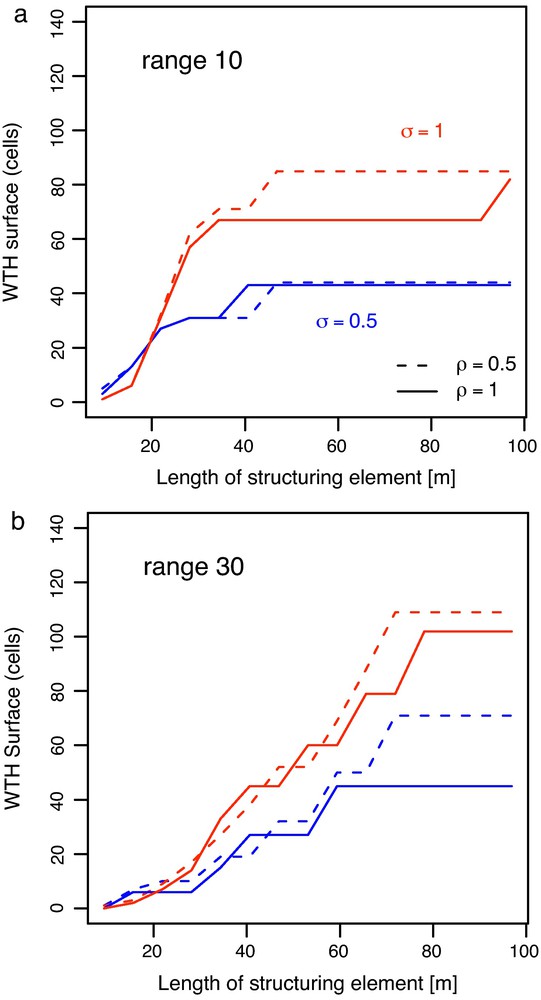
Influence on WTH of standard deviation (σlogk = 0.5 ÷ 1) and correlation coefficients ρ = 0.5 ÷ 1 for correlation lengths a = 10 (6a) and a = 30 (6b). Fig. 6. Influence de l’écart-type logarithmique (σlogk = 0, 5 ÷ 1) et du coefficient de corrélation ρ = 0, 5 ÷ 1 sur le “White Top Hat” pour deux valeurs de la portée: a = 10 (6a) et a = 30 (6b).
It should be noted that the impact of an increasing variance is to increase the extension of the fingering, which can be seen in the higher sill of the WTH, without any noticeable modification of their shape (the point of maximum slope is only slightly shifted towards the right with increasing σlogk).
Other simulations (De Lucia, 2008), not presented in this paper, showed that the influence of spatial variability of the initial mineral concentration is of secondary importance; this was observed for linear correlation coefficients between porosity and mineral concentration ranging from -1 to 1.
4.2 Kinematic dispersivity
A high macroscopic dispersivity α tends to reduce the deviation from the homogeneous behaviour, because it smoothes the local heterogeneities. This is a major effect, also larger than that of the range (Fig. 7), at least for the values chosen for α, respectively 5 and 10 length units, i.e. 0.05 and 0.1 times the size of the domain.

Influence of the dispersivity α and the range a, for a standard deviation σlogK = 1. Fig. 7. Influence de la dispersivité α et de la portée a. Ecart-type logarithmique σlogK = 1.
4.3 Kinetics
Reactions kinetics for calcite dissolution modifies the behaviours described above. With decreasing reaction rates, the deviation from a homogeneous medium increases (Fig. 8a, Da = 93.75), which becomes even more evident when compared to equilibrium.

Influence of kinetics on the remaining mineral curves for two values of the domain-averaged Damkhöler number: (8a) fast kinetics (Da = 93.75) and (8b) slow kinetics (Da = 18.75), and complementary effects of the range and dispersivity for a standard deviation σlogK = 1. Fig. 8. Influence de la cinétique sur le pourcentage de minéral restant pour deux valeurs du nombre de Damkhöler moyenné sur le domaine: (8a) cinétique rapide (Da = 93, 75) et (8b) cinétique lente (Da = 18, 75), et effet de la portée et de la dispersivité. Ecart-type logarithmique σlogK = 1. Masquer
Influence of kinetics on the remaining mineral curves for two values of the domain-averaged Damkhöler number: (8a) fast kinetics (Da = 93.75) and (8b) slow kinetics (Da = 18.75), and complementary effects of the range and dispersivity for a standard ... Lire la suite
With further decreased reaction velocities, the reactions fall below the threshold discriminating between hydrodynamically and kinetically controlled regimes, and the deviation from homogeneous behaviour gets smaller (Fig. 8b, Da = 18.75).
In the limiting case where reactions are very slow, they occur homogeneously in the whole medium, independently of flow velocities, and the simulations become very close to that of a homogeneous medium (Fig. 9).

Influence on the integral remaining mineral of the standard deviation σlogK and the range a, for dispersivity α = 5, in the case of a very slow kinetic rate (Da = 9.375). The simulation with σlogK = 1 and a = 30 did not converge, hence the truncated line in the figure. Fig. 9. Influence de l’écart-type logarithmique σlog K et de la portée a sur le pourcentage de minéral restant. Dispersivité α = 5, cas d’une cinétique très lente (Da = 9, 375). Dans le cas σlog K = 1 et a = 30, la simulation ne converge pas, d’où la troncature de la courbe. Masquer
Influence on the integral remaining mineral of the standard deviation σlogK and the range a, for dispersivity α = 5, in the case of a very slow kinetic rate (Da = 9.375). The simulation with σlogK = 1 and ... Lire la suite
4.4 Stochastic variability
The above considerations are made on the basis of just one simulation. Other simulations, not presented in this paper, suggest that such behaviour and the sensitivity to the parameters are recurring and thus trustworthy, at least from a qualitative point of view (De Lucia, 2008). Nevertheless, in order to make truly quantitative assumptions, the stochastic effect resulting from the random generation of the initial simulations has to be addressed, and the whole study should be made on the average resulting from a consistent number of independent realizations (a few dozens up to several hundreds). The problem here is the CPU-time needed for such a study, which is still a major constraint in reactive modelling. The total CPU-time of the simulations presented in this paper is of 35 days on a quad core system for approximately 120 simulations. The continual optimization of computer codes and computing infrastructures will in the very near future allow runs of such a full array of simulations, but this was not feasible at the time of this study.
Therefore, the investigation was limited to the most interesting case, i.e. the set of parameters which gave the largest deviation with respect to the homogeneous medium (a = 30, σlogK = 1, ρ = 1, in conditions of thermodynamic equilibrium). We generated a family of ten initial media, and then ran the reactive transport modelling twice on those simulations, fixing the value of dispersivity α once at 5 and then at 10. The overall results for those 2 × 10 independent realizations of porosity and permeability are shown in Fig. 10.

Stochastic variability for two families of 10 draws at dispersivity α = 10 and 5 (with fixed a, σlogK, ρ and Da). Fig. 10. Variabilité stochastique pour deux ensembles de 10 tirages et deux valeurs de la dispersivité α = 10 et 5, à a, σlog K, ρ et Da donnés.
The curves are widely scattered: the scale of such a deviation is comparable to that observed in the previous paragraphs when, for instance, different correlation lengths are compared, as in Fig. 7. Incidentally, the almost empty intersection of the two families (for two values of dispersivity) proves the discriminating power of kinematic dispersion. The WTH is considerably less sensitive to this scattering, proving that such an observable captures the qualitative behaviour of the system.
Nevertheless, this scatter does not invalidate all the comparisons made in the previous paragraphs. In fact, all simulations used in the sensitivity analysis are drawn from a unique set of random numbers, thus “filtering” the effect of random draw variability from one HYTEC simulation to another; and the same relative results are expected independently from the particular random field realization, when one compares only the effects of the parameters describing the spatial variability. This intuitive remark was confirmed in a different, non-exhaustive set of simulations, not showed in this paper, over the original square permeameter, but with a different set of random numbers, or domains twice or six times larger than the first one (De Lucia, 2008). These simulations showed that the periodical form of the reaction front, as summarized by the WTH, is independent on the ratio domain size/correlation length. On the contrary, the overall quantity of mineral in place is not able to capture the effects of spatial variability when the size of the domain increases, a clear sign of the homogenization effect obtained with a greater domain size/correlation length ratio (De Lucia, 2008).
As remarked by the reviewers, a fully quantitative description of the influence of the spatial parameters would need to be made, using a more systematic Monte-Carlo approach.
5 Conclusions
Hydrodynamics simulations coupled with reactive transport were conducted on simplified spatial discretizations of porous media and with simplified chemical reactions leading to mineral dissolution, focusing on the feedback of chemistry acting on flow and transport, especially in the case of a positive feedback (increase of porosity). It was found that, for the chosen conditions, the most important parameters explaining the difference with respect to the homogenous reference case are the correlation length of the geostatistical simulations, which controls the width of the fingering, and the kinematic dispersion, which in turn smoothes the heterogeneities. The influence of the permeability variance, and that of the correlation between porosity and permeability, are of second order, generally enhancing the effect of the correlation length.
The role of the kinetic rate is two-fold: when the reactions are limited by the transport rate (fast reactions), decreasing reaction rates amplify the divergence from the homogeneous case. As the system becomes controlled by the reaction rate (slow kinetics), the reactions occur more homogeneously throughout the whole domain, the reaction front becomes less sharp and the heterogeneities due to flow processes become less significant: the system behaves similarly to the homogeneous one.
To summarize, the most favourable conditions for developing and increasing heterogeneities are characterized by a large correlation length and a small dispersivity, associated with a strong permeability variance, a correlation porosity/permeability near 1 and flow/kinetic conditions close to the shifting point between kinetically and hydrodynamically controlled reaction rates.
Another series of test cases (not detailed in the paper; for complete reference see De Lucia, 2008) was built with a different reaction path: continuing with acidic dissolution of calcite, the precipitation of gypsum was obtained by injection of sulphuric acid. The result is a net increase of the mineral volume (molar volume 37 ml/mol for calcite versus 75 ml/mol for gypsum). As a result, the system develops negative feedback: high local permeabilities enhance the local flow, increasing the reaction, so that porosity decreases which in turn decreases the permeability. The reaction tends to stabilize the system, because of the reduction of permeability in the reactive zones. Any developing fingering triggers a local decrease in the flow velocity, which prevents it from further developing.
This work illustrates the influence of spatial variability on a reactive transport system including feedback of the chemistry acting on the hydrodynamics: development of geometrically complex interfaces, breakthrough time, and residence time. The importance of spatial variability should not be neglected in reactive transport simulations. The implications can be major, either in terms of process optimization or for risk assessment. The field of application is as broad as reactive transport per se. These applications concern long-time storage efficiency and safety, pollution characterization and subsequent natural or engineered remediation, metallogenesis, etc.
The relative influence of different parameters of the system was systematically examined. Two powerful synthesizing tools were developed, and a hierarchy of significant parameters was elaborated. However, this work is not complete, e.g. other correlation laws between porosity and permeability could be tested. Another correlation should also be addressed: mineral facies and concentration and porosity/permeability are clearly not independent in natural systems, a point that has been omitted in this study. Also, more complex and more realistic chemical systems should be considered.
The geometry of the system was minimalistic, which suited our purpose; however, the influence of the geometry should be tested on more complex and more relevant geometries; in particular, the boundary conditions may also play a major role in the dispersion of the results compared to homogeneous cases. Likewise, the choice of a geostatistical model may have a real influence on the results. A better description of a natural medium could be pursued, including multi-scale heterogeneities.
Acknowledgments
The authors want to express their gratitude to the three anonymous reviewers, whose precious advice greatly helped improve the manuscript.
1 second order stationarity means that all the first and second moments of the Random Function are constant over the domain.