A neurocomputing approach to the forecasting of monthly maximum temperature over Kolkata, India using total ozone concentration as predictor

Syam Sundar De; Goutami Chattopadhyay; Bijoy Bandyopadhyay; Suman Paul

doi:10.1016/j.crte.2011.08.002

External geophysics, climate (Aeronomy and meteorology)

A neurocomputing approach to the forecasting of monthly maximum temperature over Kolkata, India using total ozone concentration as predictor
[Approche par calcul neuronal pour la prévision de la température mensuelle maximum sur Kolkata, Inde, par utilisation de la concentration maximum d’ozone total en tant que prédicteur]

Présenté par : Michel Petit

Syam Sundar De ¹ ; Goutami Chattopadhyay ¹ ; Bijoy Bandyopadhyay ¹ ; Suman Paul ¹

¹ Centre of Advanced Study in Radio Physics and Electronics, University of Calcutta, 1, Girish Vidyaratna Lane, Kolkata 700 009, India

Comptes Rendus. Géoscience, Volume 343 (2011) no. 10, pp. 664-676.

Résumés

Anglais
Français

The association between the monthly total ozone concentration and monthly maximum temperature over Kolkata (22.56° N, 88.30° E), India, has been explored in this paper. For this, the predictability of monthly maximum temperature based on the total ozone as predictor is investigated using Artificial Neural Network. The presence of persistence and similar cyclic patterns are revealed through autocorrelation and cross-correlation coefficients. Common cycles of length 12 and 6 have been identified through periodogram. Hence, a predictive model has been generated by Artificial Neural Network in the form of Multi Layer Perceptron (MLP) using scaled conjugate gradient learning with sigmoid non-linearity. After training and testing the network, an MLP with total ozone of month n as predictor and maximum temperature of month (n + 1) as the target output is found as the best model. Performance of the model has been judged statistically. Finally, the MLP model has been compared with linear and non-linear regressions and the efficiency of MLP has been established over the regression models.

L’association entre la concentration mensuelle en ozone total et la température mensuelle maximum sur Kolkata (22,56°N ; 88,30°E), Inde, est explorée dans le travail ici présenté. Dans ce but, la prédictabilité de la température annuelle maximum basée sur l’ozone total comme prédicteur, a été examinée en utilisant le Réseau Neuronal Artificiel. La présence de persistance et de diagrammes cycliques similaires sont observés au moyen des coefficients d’autocorrélation et de corrélations croisées. Des cycles communs, de longueur comprise entre 6 et 12 ont été identifiés au moyen de périodogrammes. D’où un modèle prédictif généré par réseau neuronal artificiel sous la forme de perception multi-couche (MLP) utilisant un apprentissage de gradient conjugué à non-linéarité sigmoïde. Après avoir entraîné et testé le réseau, un modèle MLP avec l’ozone total d’un mois n en tant que prédicteur et la température maximum du mois (n + 1) en tant que sortie de cible, a été estimé comme étant le meilleur modèle. La performance du modèle a été jugée statistiquement. Enfin, le modèle a été comparé avec les régressions linéaires et non-linéaires, et l’efficacité du MLP par rapport aux modèles de régression a été bien établie.

Métadonnées

Reçu le : 2011-02-04
Accepté le : 2011-08-29
Publié le : 2011-10-01

DOI : 10.1016/j.crte.2011.08.002

Keywords: Monthly total ozone concentration, Monthly maximum temperature, Artificial Neural Network, Multilayer perceptron
Mot clés : Concentration mensuelle d’ozone total, Température mensuelle maximum, Réseau neuronal artificiel, Perception multi-couche

Affiliations des auteurs :

Syam Sundar De ¹ ; Goutami Chattopadhyay ¹ ; Bijoy Bandyopadhyay ¹ ; Suman Paul ¹

¹ Centre of Advanced Study in Radio Physics and Electronics, University of Calcutta, 1, Girish Vidyaratna Lane, Kolkata 700 009, India

@article{CRGEOS_2011__343_10_664_0,
     author = {Syam Sundar De and Goutami Chattopadhyay and Bijoy Bandyopadhyay and Suman Paul},
     title = {A neurocomputing approach to the forecasting of monthly maximum temperature over {Kolkata,} {India} using total ozone concentration as predictor},
     journal = {Comptes Rendus. G\'eoscience},
     pages = {664--676},
     publisher = {Elsevier},
     volume = {343},
     number = {10},
     year = {2011},
     doi = {10.1016/j.crte.2011.08.002},
     language = {en},
}

TY  - JOUR
AU  - Syam Sundar De
AU  - Goutami Chattopadhyay
AU  - Bijoy Bandyopadhyay
AU  - Suman Paul
TI  - A neurocomputing approach to the forecasting of monthly maximum temperature over Kolkata, India using total ozone concentration as predictor
JO  - Comptes Rendus. Géoscience
PY  - 2011
SP  - 664
EP  - 676
VL  - 343
IS  - 10
PB  - Elsevier
DO  - 10.1016/j.crte.2011.08.002
LA  - en
ID  - CRGEOS_2011__343_10_664_0
ER  -

%0 Journal Article
%A Syam Sundar De
%A Goutami Chattopadhyay
%A Bijoy Bandyopadhyay
%A Suman Paul
%T A neurocomputing approach to the forecasting of monthly maximum temperature over Kolkata, India using total ozone concentration as predictor
%J Comptes Rendus. Géoscience
%D 2011
%P 664-676
%V 343
%N 10
%I Elsevier
%R 10.1016/j.crte.2011.08.002
%G en
%F CRGEOS_2011__343_10_664_0

Syam Sundar De; Goutami Chattopadhyay; Bijoy Bandyopadhyay; Suman Paul. A neurocomputing approach to the forecasting of monthly maximum temperature over Kolkata, India using total ozone concentration as predictor. Comptes Rendus. Géoscience, Volume 343 (2011) no. 10, pp. 664-676. doi : 10.1016/j.crte.2011.08.002. https://comptes-rendus.academie-sciences.fr/geoscience/articles/10.1016/j.crte.2011.08.002/

Version originale du texte intégral

1 Introduction

Suitability of stratospheric predictors in generating extended range forecast of tropospheric variables is well documented in the literature (Baldwin et al., 2003; Jung and Barkmeijer, 2006). Most of the energy that drives the climate system comes from the sun and variations in solar radiation on several timescales are linked with substantial variations of Earth's climate. Because of the absorption of ultraviolet (UV) radiation by ozone in the stratosphere, its concentration varies with the intensity of UV radiation (Alexandris et al., 1999, Katsambas et al., 1997). Ozone variations have a direct radiative impact on the stratosphere and troposphere, and it has been observed that the atmospheric temperatures are broadly consistent with the radiative processes (Baldwin and Dunkerton, 2005). Based on the concept of general circulation model (GCM), it is shown that the changes in tropospheric circulation and temperature are produced in response to stratospheric thermal perturbations (Simpson et al., 2009). Several authors investigated the variability of stratospheric ozone and temperature on monthly to inter-annual timescales (Fusco and Salby, 1999; Kiladis et al., 2006; Randel and Cobb, 1994).

Ozone plays a fundamental role in controlling the chemical composition and climate of the troposphere (Cracknell and Varotsos, 1994; Kondratyev and Varotsos, 1996; Varotsos, 1987, 2002). Tropospheric photochemistry is initiated by photolysis of ozone, which leads to the formation of hydroxyl radical. Absorption of thermal radiation by ozone influences the energy budget of the troposphere (Kondratyev and Varotsos, 1995; Logan and Kirchhoff, 1986). In an analysis of mean-monthly temperature and total ozone data, Angell and Korshover (1964) suggested that quasi-biennial oscillations extend to the polar latitudes of both hemispheres. Much of the observed variability of stratospheric ozone and temperature on monthly to inter-annual timescales is attributable to trend like changes or to forced variations with specified timescales (Cracknell and Varotsos, 1994; Randel and Cobb, 1994; Varotsos, 2004). Correlations between ozone and temperature are commonly used to investigate the photochemical and dynamical aspects of satellite-derived ozone data. The dynamical contributions to the ozone temperature correlations are examined by Rood and Douglass (1985). Sensitivity of ozone to temperature in the upper stratosphere and lower mesosphere is investigated by Froidevaux et al. (1989). Shibata and Deushi (2005) investigated the radiative effect of ozone on the quasi-biennial oscillation with a chemistry-climate model. The changes in temperature have an impact on ozone chemistry in the stratosphere, which will give feedback on temperature, since ozone itself is an absorbing gas. Changes in stratospheric ozone will also alter the radiation field at the lower height levels, thus affecting the dynamics and chemistry down into the troposphere (Shindell et al., 1998). From the results of a global climate model including an interactive parameterization of stratospheric chemistry, Shindell et al. (1998) showed how upper stratospheric ozone changes may amplify the 11-year solar cycle irradiance changes to affect the climate.

It is known that the effect of total ozone (TO), which is comprised of the tropospheric and stratospheric ozone contents (Cracknell and Varotsos, 1995; Varotsos et al., 1995), has significant effects on the climatic condition over the Indian subcontinent. The TO variability is mainly dominated by annual cycles, quasi-biennial oscillations (QBO), El Niño Southern Oscillation (ENSO) and solar cycle (Cracknell and Varotsos, 1995; Varotsos et al., 1994). A significant negative correlation between TO and QBO has been observed for three Indian stations: New Delhi, Varanasi, and Pune, and positive correlation for Kodaikanal station (Londhe et al., 2003). All the stations showed significant positive correlations between TO and solar flux. It was observed by Hingane (1990) that the appearance of minima in total ozone over the subtropical belt of the Indian subcontinent may be the result of some unique signatures of thermal and dynamic processes appearing in that region. The association between the monsoon circulation and TO over India was studied by Londhe et al. (2005). Due to the non-linearity of ozone concentrations and the complex interactions between meteorological variables and ozone, the development of non-linear models like Artificial Neural Network (ANN) (Gardner and Dorling, 1998, 2000), a potent mathematical tool for modelling non-linear geophysical processes, has gained the attention of several researchers working in the area of forecasting tropospheric ozone (e.g. Abdul-Wahab and Al-Alawi, 2002; Chaloulakou et al., 2003; Clark and Karl, 1982; Corani, 2005; Gardner and Dorling, 1998, 2000; Gómez-Sanchis et al., 2006; Hsieh and Tang, 1998; Salazar-Ruiz et al., 2008; Wang et al., 2003). Comrie (1997) compared the performance of ANN with conventional regression method in forecasting the surface ozone concentration and established the supremacy of the ANN over conventional regression. In a comparative study based on a wide set of forecast quality measures, Chaloulakou et al. (2003) indicated that the ANNs provide better estimates of ozone concentrations, whilst the more often used linear models are less efficient at accurately forecasting high ozone concentrations. Sousa et al. (2007) studied a comparison between ANN and multiple linear regression by removing the effect of multicollinearity by means of principal components and found that ANN equipped with principal component analysis performed significantly better than the multiple linear regression model. Salazar-Ruiz et al. (2008) compared the performance of different types of ANN with Ridge regression and obtained results with similar margins of errors. Although the application of ANN in forecasting tropospheric ozone is available in handful, the application of ANN is not so frequent in modelling and forecasting the TO, which is characterized by immense non-linearity and complexity (Chattopadhyay and Chattopadhyay, 2008a, 2010a; Koçak et al., 2000). Chattopadhyay and Chattopadhyay (2009a, 2009b, 2010b) implemented ANN in modelling TO. Although the study of Chattopadhyay and Chattopadhyay (2009a) was made in a multivariate environment, the studies of Chattopadhyay and Chattopadhyay (2009b, 2010b) were based on univariate approaches where autoregressive ANN models were generated and compared with autoregressive moving average and autoregressive integrated moving average models.

The ANN applications discussed in the last paragraph were involved with prediction of ozone or TO based on other meteorological parameters or the past values of TO time series. However, the present study deviates from the aforesaid studies in the sense that instead of predicting TO using meteorological parameters, it has adopted TO as the predictor to generate a predictive model for surface temperature, which is a vital parameter for various meteorological processes. The average air temperature at the surface of the Earth is a frequently used parameter for sensing the state of a climatic system (Ceschia et al., 1994; Chattopadhyay et al., 2010a, 2010b). Necessity for predicting the surface temperature has been emphasized in various papers (e.g. Hussain, 1984; Rehman et al., 1990; Said, 1992; Tasadduq et al., 2002). The study area, Kolkata, of the present paper belongs to Gangetic West Bengal, which is characterized by severe pre-monsoon (March–May) thunderstorms and heavy summer-monsoon (June–September) rainfall. Role of temperature in the genesis of thunderstorm is studied in Haklander and Delden (2003), Huntrieser et al. (1997), Schmeits et al. (2005) and the role of temperature in rainfall is discussed in Elliott and Angell (1987), Kumar et al. (1997, 1999), Liu and Yanai (2001). The primary objective of the present article is to discern how the monthly maximum temperature (Tmax) over Kolkata is associated with the monthly TO. The newness of the present study can be summarized as follows:

The organization of the rest of the article is as follows: in Section 2, the data under consideration are analyzed through autocorrelation function, cross-correlation function, and through periodogram method of analysis. In Section 3, ANN models are generated to forecast Tmax based on TO as predictor. In Section 4, various regression models are generated and finally, it has been examined whether an extended range forecast of monthly maximum temperature can be estimated using ANN with its non-linear methodology.

2 Different statistical analyses of the data

2.1 Data

In the present paper, the data are derived from the measurements made by the Earth Probe Total Ozone Mapping Spectrometer (EP/TOMS). The EP/TOMS experiment provides measurements of the Earth's total column ozone by measuring the backscattered Earth radiance in the six 1 nm bands (NASA, 1998). The total ozone (TO) data are available at ftp://jwocky.gsfc.nasa.gov/pub/eptoms/data/overpass/OVP075_epc.txt. In this paper, January 1997 to December 2002 monthly TO data over Kolkata has been utilized. The corresponding monthly maximum temperature (Tmax) data for Kolkata have been collected from the website of India Waterportal (http://www.indiawaterportal.org/taxonomy/term/1216). The time series of Tmax and TO are plotted on Fig. 1.

Fig. 1
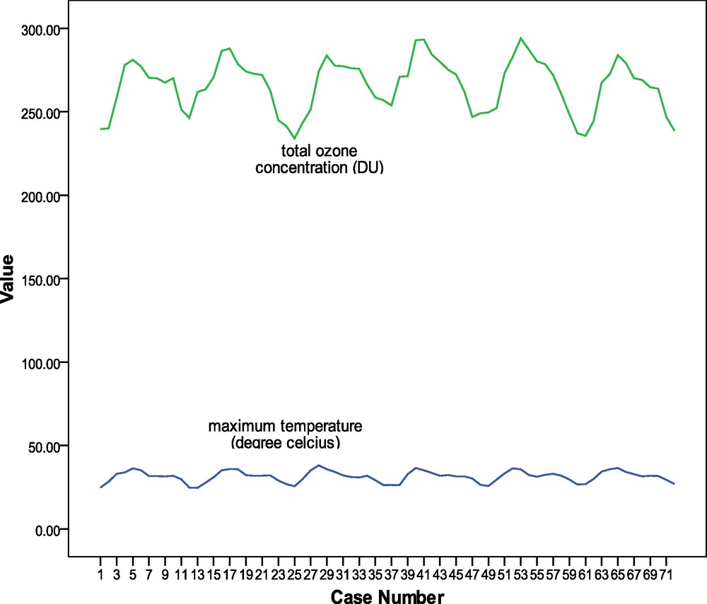
Time series of monthly maximum temperature (°C) and monthly total ozone concentration (DU) over Kolkata during the period 1997–2002.
Séries temporelles de température (°C) mensuelle maximum et de concentration (DU) mensuelle d’ozone total sur Kolkata, pendant la période 1997–2002.

2.2 Autocorrelation structure analysis

Atmospheric variables often exhibit statistical dependence with their own past or future values. In the terminology of the atmospheric sciences, this dependence through time is usually known as persistence. Persistence can be defined as the existence of (positive) statistical dependence among successive values of the same variable, or among successive occurrences of a given event (Wilks, 2006). Positive dependence means that large values of the variable tend to be followed by relatively large values, and small values of the variable tend to be followed by relatively small values. The persistence is measured by means of autocorrelation coefficients computed as (Wilks, 2006).

r_{k} = \frac{C o v [(\bar{x} (n - k)), (\underline{x} (n - k))]}{\sqrt{V a r i a n c e ((\bar{x} (n - k)))} \sqrt{V a r i a n c e ((\underline{x} (n - k)))}}

(1)

where

\bar{x} (n - k)

and

\underline{x} (n - k)

denote the average of first (n – k) and last (n – k) data values of the time series. Examples of autocorrelation function analysis in climatological study include the works of Sivakumar (2001), Daoud et al. (2003), Krzysztofowicz and Evans (2008). From the autocorrelation function of the monthly TO displayed on Fig. 2, it is found that lag1 autocorrelation is 0.757, which indicates persistence in the time series and lag12 autocorrelation coefficient showed 0.622. In the negative side, the most negative autocorrelation coefficients are occurring at lag6 and lag18, which are –0.619 and –0.513 respectively. This clearly indicates the presence of annual cycle within the time series.

Fig. 2
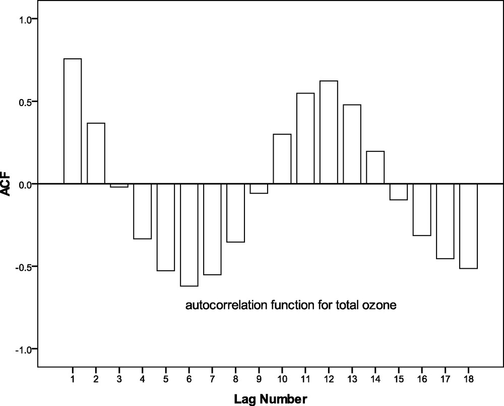
Autocorrelation function for the monthly total ozone concentration over Kolkata during the period 1997–2002.
Fonction d’autocorrélation pour la concentration mensuelle d’ozone total sur Kolkata, pendant la période 1997–2002.

In the case of Tmax over the study zone, it is found from Fig. 3, that the lag1 autocorrelation is 0.684, which indicates existence of significant persistence within the time series. At lag12, it is 0.772. However, in the negative side, the autocorrelation coefficients are not as large as they are in the case of TO. From Figs. 2 and 3, a similarity is observed between the TO and Tmax over Kolkata. Both the time series are completing a cycle in 12 months. Moreover, in both the cases, lag1 and lag12 autocorrelation coefficients are significantly high.

Fig. 3
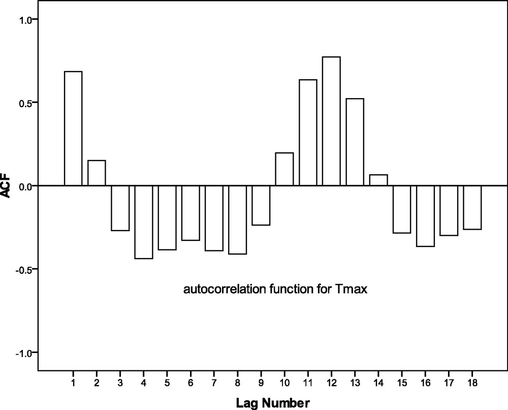
Autocorrelation function for the monthly maximum temperature over Kolkata during the period 1997–2002.
Fonction d’autocorrélation pour la température mensuelle maximum sur Kolkata, pendant la période 1997–2002.

The search for the relationships usually involves the calculation of a sample cross-correlation function (CCF) for the pairs of time series (Chang et al., 1997; Kripalani and Kumar, 2004). Considering the CCF between monthly TO and Tmax time series on Fig. 4, it is observed that the cross-correlation coefficients lie between –0.6 and 0.8. It should be noted that dominant negative and positive cross-correlation coefficients (CC) are existing. The pattern of CCF for the lags –7 to –3 and 3 to 7 are having similar patterns with high negative CC at the lags –5 and 7. A high positive CC is occurring at lag 0. It may be further noted that like the ACF, the CCF is also exhibiting a sinusoidal pattern. The CCs are prominent at 99% level of significance. From these observations, it can be interpreted that the Tmax and TO show significant degree of similarity in their temporal variation. Finally, it is observed that the CCF is symmetric about the horizontal axis representing the lags as negative and positive levels. The stability or symmetry of the CCF about the horizontal axis indicates a stable relationship between TO and Tmax. Hence, it is possible to generate a predictive model for Tmax using TO as predictor.

Fig. 4
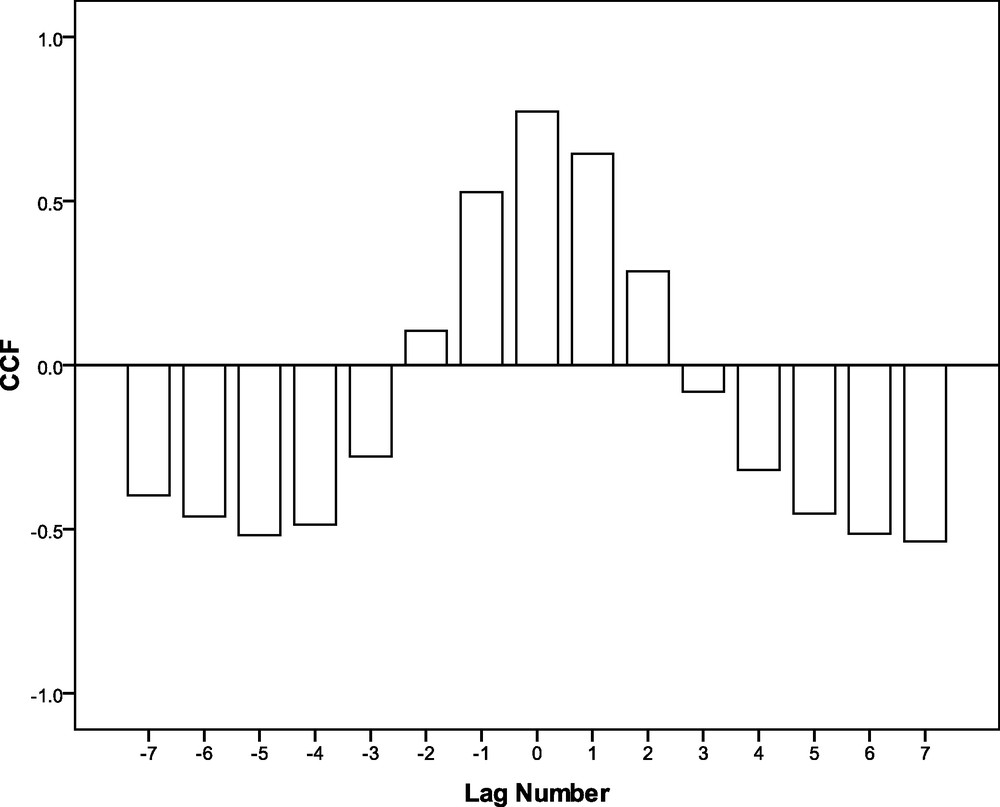
Cross-correlation coefficients for the monthly total ozone concentration and monthly maximum Temperature over Kolkata during the period 1997–2002.
Coefficients de corrélations croisées pour la concentration mensuelle d’ozone total et la température mensuelle maximum sur Kolkata, pendant la période 1997–2002.

2.3 Periodogram analysis

There have been literally thousands of attempts to find cycles in meteorological phenomena. Application of periodogram method in the analysis of time series of climatological data is well discussed in various papers (Gil-Alana, 2005; Marr and Harley, 2002; Prouse and Ervin, 1935; Seleshi et al., 1994; Vyushin et al., 2007). Any data series consisting of n points can be represented by adding together a series of n/2 harmonic functions as (Wilks, 2006).

y_{t} = \bar{y} + \sum_{k = 1}^{n / 2} \{A_{k} \cos [\frac{2 π k t}{n}] + B_{k} \sin [\frac{2 π k t}{n}]\}

(2)

where A_k and B_k are Fourier coefficients. The advantage of this perspective is that it allows us to see separately the contributions to a time series that are made by processes varying at different speeds, that is, by processes operating at a spectrum of different frequencies (Wilks, 2006). The characteristics of a time series are Fourier-transformed into the frequency domain and are most often examined graphically, using a plot known as the periodogram, or Fourier line spectrum. The plot of spectrum consists of

C_{k} = \sqrt{{A_{k}}^{2} + {B_{k}}^{2}}

along the vertical axis and period of the kth harmonic

τ_{k} = \frac{n}{k}

along the horizontal axis (Wilks, 2006). In the present work, periodograms of monthly TO and monthly Tmax time series are presented on Figs. 5 and 6. It is interesting to note that the periodogram of TO time series reflects some of the features of the Tmax periodogram. In the case of TO, the maximum density 12840.193 corresponds to the period 12 and in the case of Tmax, the highest density 513.428 corresponds to the period 12. Thus, the common spectrum of length 12 is available in both TO and Tmax time series. Furthermore, it should be noted that at the period 6, both of the time series are having next maximum spectral density. This further indicates the similarity in the patterns of the two time series under consideration.

Fig. 5
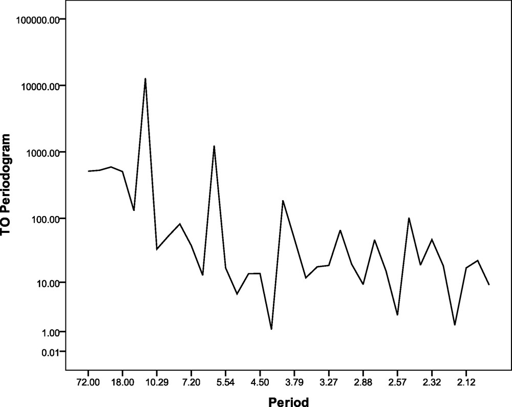
Periodogram analysis for the monthly total ozone time series over Kolkata during the period 1997–2002.
Périodogramme pour la série temporelle d’ozone total mensuel sur Kolkata, pendant la période 1997–2002.

Fig. 6
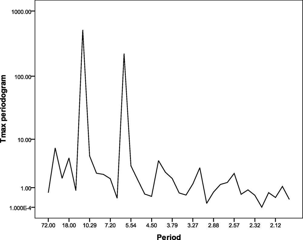
Periodogram analysis for the monthly maximum temperature time series over Kolkata during the period 1997–2002.
Périodogramme pour la série temporelle de température mensuelle maximum sur Kolkata, pendant la période 1997–2002.

In the subsequent sections, it will be examined whether a predictor-predictand relationship exists between TO and Tmax. To do the same, one has to examine whether Tmax of the given month can be estimated on the basis of TO of the previous months. The ANN would be implemented for this purpose. A brief overview and implementation procedure of ANN would be elaborated in the subsequent sections.

3 Artificial Neural Networks: a brief review

Fundamental development in the area of feed forward ANN during the period 1960–1990 was reviewed extensively by Widrow and Lehr (1990). Introduction of back propagation algorithm (Rumelhart and McClelland, 1986) opened up new avenues to the application of ANN in modelling various time series problems (Hsieh and Tang, 1998). In the simplest form, backpropagation training begins by presenting an input pattern vector to the network, sweeping forward through the system to generate an output response vector, and computing the errors at each output (Widrow and Lehr, 1990). The next step involves sweeping the effect of the errors backward. Finally, the weights are updated based on the corresponding error gradient. A wide review of application of backpropagation learning to the atmospheric problems is available in Gardner and Dorling (1998). Maier and Dandy (2000) presented an extensive review of the application of ANN in predicting hydrological time series. Several applications of ANN are available in meteorological forecasting problems like thunderstorm (Manzato, 2005; Marzban and Stumpf, 1996), rainfall (Chattopadhyay and Chattopadhyay, 2010a; Kuligowski and Barros, 1998), tide (Leea and Jeng, 2002), groundwater level (Coulibaly et al., 2001), evapotranspiration (Zanetti et al., 2007) etc. In Section 1, various examples of applications of ANN in modeling and forecasting of tropospheric ozone are discussed.

The present paper applies ANN in the form of multilayer perceptron (MLP) (Gardner and Dorling, 1998; Haykin, 2008; Rojas, 1996). In MLP, each network consists of several simple processors called neurons, or cells, which are highly interconnected and arranged in several layers. There are three basic types of layers: input layer, hidden layer(s), and output layer. Input and output layers are connected through hidden layer(s). There may be one to several hidden layers in between input and output layers. In mathematical form, the adaptive procedure of a feed forward MLP can be presented as (Kamarthi and Pittner, 1999).

w_{k + 1} = w_{k} + η d_{k}

(3)

Here, w_k denotes the weights to the ANN. The direction vector d_k is the negative gradient of the output error function E, and is given by

d_{k} = - \nabla E (w_{k})

(4)

The backpropagation algorithm in which the weights of the network are updated immediately after the presentation of each pair of input and target output is called the sequential learning. The other learning procedure in which the whole training set is considered as a batch is called the batch learning. Silverman and Dracup (2000) identified the advantages of ANN over conventional statistical methods as:

• a priori knowledge of the underlying process is not required;
• existing complex relationships among the various aspects of the process under investigation need not be recognized;
• constraints and a priori solution structures are neither assumed nor enforced.

4 Implementation of Artificial Neural Network

Several conjugate gradient algorithms are there in the literature of ANN learning. Johansson et al. (1990) described in detail the theory of general conjugate gradient methods and how to apply the methods in feed-forward ANNs. Møller (1993) introduced a variation of a conjugate gradient method (Scaled Conjugate Gradient, SCG), which avoids the line-search per learning iteration by using a Levenberg-Marquardt approach in order to scale the step size. The Conjugate Gradient methods choose the search direction and the step size more carefully by using information from the second order approximation (Møller, 1993).

E (w + y) \approx E (w) + E^{'} {(w)}^{T} y + \frac{1}{2} y^{T} E^{″} (w) y

(5)

where w is the weight vector, which is a vector in the real Euclidean space R^N, where N is the number of weights and biases in the network. A basis of R^N is chosen as the conjugate system

\{p_{1}, p_{2}, \dots, p_{N}\}

. In SCG, a Lagrangian multiplier λ_k was introduced by Møller (1993) to regulate the indefiniteness of the Hessian matrix E”(w) and the second order information was set as

s_{k} = \frac{E^{'} (w_{k} + σ_{k} p_{k}) - E^{'} (w_{k})}{σ_{k}} + λ_{k} p_{k}, with, 0 < σ_{k} < < 1

(6)

Since its introduction, the SCG has been used in several ANN applications for geophysical problems (e.g. Abraham and Nath, 2001; Khan and Coulibaly, 2006). In the present paper, SCG has been applied with sigmoid activation function $f (x) = \frac{1}{1 + e^{- x}}$ . Advantage of the sigmoid function is the form of its derivative. Gardner and Dorling (1998) discussed the advantage of this activation. In Any model development process data pre-processing can have a signiﬁcant effect on model performance. As the outputs of the logistic transfer function are between 0 and 1, the data are generally scaled in the range 0.1–0.9 or 0.2–0.8. If the values are scaled to the extreme limits of the transfer function, the size of the weight updates is extremely small and ﬂatspots in training are likely to occur. Before developing the proposed ANN model for prediction of Tmax based on TO concentration, the data are scaled to [0.1,0.9] to avoid the asymptotic effect caused by the sigmoidal activation function. The scaling is done by using the transformation

x_{t r a n s f o r m e d} = x_{\min} + {0.8}^{- 1} (x - 0.1) (x_{\max} - x_{\min})

(7)

Minimization of mean squared error is taken as the stopping criterion for the ANN model. It is common practice to split the available data into two sub-sets; a training set and an independent validation set (Maier and Dandy, 2000). Typically, ANNs are unable to extrapolate beyond the range of the data used for training. One method, which maximizes utilization of the available data, is the holdout method (Maier and Dandy, 2000) that we have used in this article. The basic idea is to withhold a small subset of the data for validation and to train the network on the remaining data. Once the generalization ability of the trained network has been obtained with the aid of the validation set, a different subset of the data is withheld and the above process is repeated. Different subsets are withheld in turn, until the generalization ability has been determined for all of the available data (Maier and Dandy, 2000). In the present paper, we have divided the dataset into the ratio of 67:33 in order to use two third of the entire dataset as the training set and the remaining one third as the test set. As the generalization ability is determined for all of the available data, the prediction performance is measured by Willmott's index (WI) (Comrie, 1997; Chattopadhyay and Chattopadhyay, 2010b; Willmott, 1982) given by

WI = 1 - [\sum_{i = 1}^{N} {(P_{i} - O_{i})}^{2} / \sum_{i = 1}^{N} {(|P_{i} - \bar{O}| + |O_{i} - \bar{O}|)}^{2}]

(8)

The usefulness of WI in meteorological modeling is discussed in Chattopadhyay and Chattopadhyay (2008b).

In the present ANN modeling problem with SCG learning, the data set contains the TO and Tmax data pertaining to January 1997 to December 2002. Thus, in monthly scales, there are 72 data points. In this data set, ANN model in the form of MLP will be generated. The first target is to examine whether it is possible to estimate Tmax of a given month using TO concentration of the immediately previous month. In this case, there would be 71 input patterns in the MLP model. The order of the input matrix would be (71 × 2). The first column of the input matrix corresponds to TO and the second column corresponds to the observed monthly Tmax, which is the target output of this supervised learning methodology. The MLP is learned through SCG with single hidden layer and the optimum size of the hidden layer, i.e., the optimum number of nodes in the hidden layer is recorded. After training and testing, the model is validated over the entire set of target outputs. The WI is found to be 0.863 and the value of R² is 0.560. The actual Tmax and those predicted by this ANN model are plotted as line diagram in Fig. 7a. In this line diagram, it is observed that in some of the test cases, the actual and predicted values are almost coincident. In Fig. 7b, a scatterplot is presented to view the degree of linearity between the actual and predicted Tmax. A prominent positive slope is discernible in the scatterplot that indicates a good positive association between the actual and predicted Tmax. Calculating the percentage error of prediction in the test cases, it is found that in 83.1% and 70.4% test cases, the errors of predictions are below 5% and 2.5%, respectively. Thus, the predictions yields for 5% and 2.5% acceptable errors are 0.831 and 0.704 respectively. This further proves the goodness of fit of the ANN model in the form of MLP. The Pearson correlation coefficient between actual and predicted values is 0.748. From the above observation it is felt that it is possible to predict the Tmax over Kolkata for a given month predicted by the TO concentration of the immediately previous month. The WI and R² values from this MLP model are presented pictorially in Fig. 9 along with those obtained from regression models, to be discussed in the next section.

Fig. 7
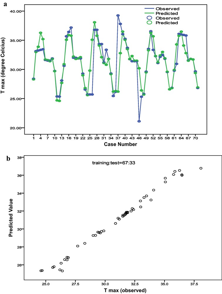
Diagrams showing the association between the actual monthly maximum temperature (̊C) (Tmax) and those predicted by multilayer perceptron model. The line diagram is plotted in 7a and scatterplot is presented in 7b.
Diagrammes montrant l’association entre température (̊C) mensuelle maximum actuelle (Tmax) et celle prédite par le modèle perception multi-couche. Diagramme linéaire en 7a et en nuage de points en 7b.

Fig. 9
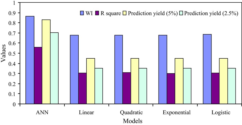
Values of different statistics measuring the suitability of different models in predicting the monthly Tmax over Kolkata based on total ozone as predictor.
Valeurs de différentes statistiques mesurant l’harmonisation des différentes méthodes dans la prédiction de la température mensuelle maximum sur Kolkata, sur la base de l’ozone total comme prédicteur.

A second model is generated by incorporating one more predictor in input matrix for the MLP. In this model, TO of months n and (n + 1) would be used to predict the Tmax of month (n + 2). Dividing the entire input matrix into training and test cases as above and implementing the identical training and test methodology, we generate the prediction model. In this case, WI is 0.866 and R² is 0.564. The WI and R² for the second model are almost equal to those of the first model. This indicates that the two models are of almost equal prediction capacity. However, the first model requires less number of predictors and hence it is more acceptable than any other model of similar prediction capacity and dependent on more number of predictors.

5 Comparison with regressions

In the present section, the performance of the first MLP model is compared with linear as well as non-linear regression models. Superiority of MLP in ozone forecasting over multiple linear regression is established in Agirre-Basurkoa et al. (2006). Non-linear regression models are chosen as quadratic regression, exponential regression and logistic regression. The regression equations are found to be as follows (Abdul-Wahab and Al-Alawi, 2002; Chattopadhyay et al., 2010a, 2010b;Comrie, 1997; Manel et al., 1999):

T \max {(n + 1)}_{l i n e a r} = 0.0948 + 0.1178 * T O (n)

(9)

T \max {(n + 1)}_{q u a d r a t i c} = 50.3484 - 0.2650 * T O (n) + 0.0007 * {(T O (n))}^{2}

(10)

T \max {(n + 1)}_{\exp o n e n t i a l} = 10.9810 * \exp (0.0039 * T O (n))

(11)

T \max {(n + 1)}_{\log i s t i c} = \frac{1}{0.0911 * {0.9961}^{T O (n)}}

(12)

The coefficients of determination R² for the above four regression models are computed as 0.306, 0.309, 0.311 and 0.322, respectively. For the above models, WI is calculated and the values are found to be 0.676, 0.678, 0.680 and 0.687, respectively. The line diagram presented on Fig. 8 shows the actual and predicted Tmax values. The line diagram shows that the linear as well non-linear regression equations captured the pattern of the observed Tmax time series. However, they are unable to yield predictions very close to the actual Tmax values especially when the Tmax value is very low or very high. Therefore, it may be concluded that the linear or non-linear regressions are unable to predict the extreme Tmax cases. The WI and R² values corresponding to the regression models are presented on Fig. 9. It is observed from the above WI and R² values that logistic regression performs better than the other three regression models. The prediction yields for the regression models are also presented in Fig. 9. It is observed that in all the regression models the prediction yields are below the ANN model when 5% and 2.5% error of prediction are allowed.

Fig. 8
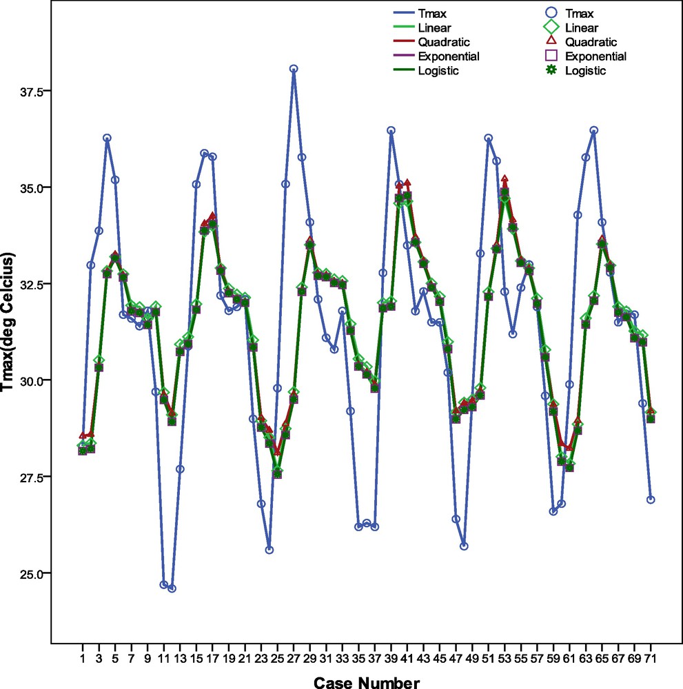
Diagram showing the association between the actual monthly Tmax (°C) and that predicted by conventional Regression model.
Diagramme montrant l’association entre la température mensuelle maximum actuelle Tmax (°C) et celle prédite par le modèle de régression conventionnel.

From the above discussion, supremacy of ANN over linear and non-linear regression models is established. To compare their performance in extreme cases, the percentage of error (PE) of prediction for the months having Tmax ≥ 35 °C and ≤ 25 °C are calculated for the first ANN model and the four regression models explained above. The PE are presented on Fig. 10, which shows that in 12, out of 16 cases, the PE produced by ANN lies below those produced by regression models. This established that ANN has higher potential than the regression models to make prediction of extremely high or low Tmax situations over the study zone.

Fig. 10
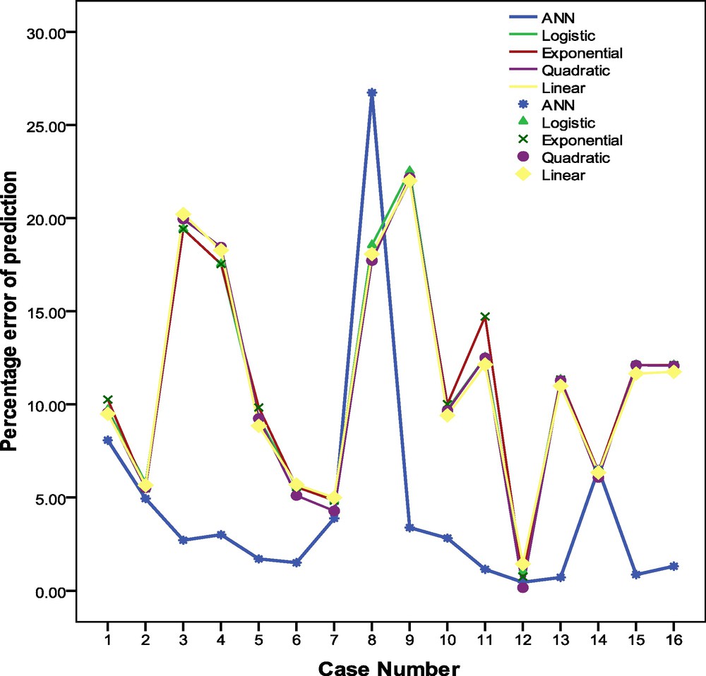
Schematic showing the percentage errors of prediction for the months in which Tmax ≥ 35 °C or Tmax ≤ 25 °C over Kolkata.
Diagramme montrant les erreurs en pour cent de prédiction pour les mois pendant lesquels Tmax ≥ 35 °C ou Tmax ≤ 25 °C sur Kolkata.

6 Conclusion

In the present article, an attempt has been made to analyze the monthly maximum temperature over Kolkata using monthly total ozone concentration as predictor. The interrelation between the predictors and the predictand has been investigated through autocorrelation, cross-correlation, and periodogram. Two ANN models have been generated in the form of MLP using scaled conjugate gradient learning with sigmoid activation function. The Willmott's indices of two MLP models are 0.863 and 0.866, respectively. The Willmott's index for the second model is almost equal to that of the first model. This indicates that the two models are of almost equal prediction capacity. However, the first model requires less number of predictors and hence it is more acceptable than any other model of similar prediction capacity and dependent on more number of predictors. To examine the skillfulness of the first MLP model, its performance has been finally compared with linear regression model and non-linear regression models in the forms of quadratic, exponential and logistic regression and the efficiency of the first model has been established. The conclusion is that, the first MLP model has considerable potential for estimating monthly Tmax using monthly total ozone concentration as predictor.

Acknowledgements

The authors acknowledge with thanks the financial support from Indian Space Research Organization (ISRO) through S.K. Mitra Centre for Research in Space Environment, University of Calcutta, Kolkata, India for carrying out the study.

Bibliographie

[Abdul-Wahab and Al-Alawi, 2002] S.A. Abdul-Wahab; S.M. Al-Alawi Assessment and prediction of tropospheric ozone concentration levels using artificial neural networks, Environ. Model. Softw., Volume 17 (2002), pp. 219-228

[Abraham and Nath, 2001] A. Abraham; B. Nath A neuro-fuzzy approach for modelling electricity demand in Victoria, Appl. Soft Comput., Volume 1 (2001), pp. 127-138

[Agirre-Basurkoa et al., 2006] E. Agirre-Basurkoa; G. Ibarra-Berastegib; I. Madariaga Regression and multilayer perceptron-based models to forecast hourly O₃ and NO₂ levels in the Bilbao area, Environ. Model. Softw., Volume 21 (2006), pp. 430-446

[Alexandris et al., 1999] D. Alexandris; C. Varotsos; K.Y. Kondratyev; G. Chronopoulos On the altitude dependence of solar effective UV. Physics and Chemistry of the Earth Part C, Solar Terrestial Planetary Sci., Volume 24 (1999), pp. 515-517

[Angell and Korshover, 1964] J.K. Angell; J. Korshover Quasi-Biennial variations in temperature, total ozone, and tropopause height, J. Atmos. Sci., Volume 21 (1964), pp. 479-492

[Baldwin et al., 2003] M.P. Baldwin; D.B. Stephenson; D.W.J. Thompson; T.J. Dunkerton; A.J. Charlton; A. O’Neill Stratospheric memory and skill of extended-range weather forecasts, Science, Volume 301 (2003), pp. 636-640

[Baldwin and Dunkerton, 2005] M.P. Baldwin; T.J. Dunkerton The solar cycle and stratosphere–troposphere dynamical coupling, J. Atmos. Solar Terrestrial Phys., Volume 67 (2005), pp. 71-82

[Ceschia et al., 1994] M. Ceschia; A. Linussio; S. Micheletti Trend analysis of mean monthly maximum and minimum surface temperatures of the 1951–1990 period in Friuli-Venezia Giulia, Il Nuovo Cimento, Volume 17 (1994), pp. 511-521

[Chaloulakou et al., 2003] A. Chaloulakou; M. Saisana; N. Spyrellis Comparative assessment of neural networks and regression models for forecasting summertime ozone in Athens, Sci. Total Environ., Volume 313 (2003), pp. 1-13

[Chang et al., 1997] P. Chang; L. Ji; H. Li A decadal climate variation in the tropical Atlantic Ocean from thermodynamic air–sea interactions, Nature, Volume 385 (1997), pp. 516-518

[Chattopadhyay and Chattopadhyay, 2008a] G. Chattopadhyay; S. Chattopadhyay A probe into the chaotic nature of total ozone time series by correlation dimension method, Soft Comput., Volume 12 (2008), pp. 1007-1012

[Chattopadhyay and Chattopadhyay, 2008b] S. Chattopadhyay; G. Chattopadhyay Comparative study among different neural net learning algorithms applied to rainfall time series, Meteorological Appl., Volume 15 (2008), pp. 273-280

[Chattopadhyay and Chattopadhyay, 2009a] G. Chattopadhyay; S. Chattopadhyay Predicting daily total ozone over Kolkata, India: skill assessment of different neural network models, Meteorological Appl., Volume 16 (2009), pp. 179-190

[Chattopadhyay and Chattopadhyay, 2009b] G. Chattopadhyay; S. Chattopadhyay Autoregressive forecast of monthly total ozone concentration: a neurocomputing approach, Comput. Geosci., Volume 35 (2009), pp. 1925-1932

[Chattopadhyay and Chattopadhyay, 2010a] G. Chattopadhyay; S. Chattopadhyay Univariate approach to the monthly total ozone time series over Kolkata, India: autoregressive integrated moving average (ARIMA) and autoregressive neural network (AR-NN) models, Intern. J. Remote Sensing, Volume 31 (2010), pp. 575-583

[Chattopadhyay and Chattopadhyay, 2010b] S. Chattopadhyay; G. Chattopadhyay Univariate modelling of summer-monsoon rainfall time series: comparison between ARIMA and ARNN, C. R. Geoscience, Volume 342 (2010), pp. 100-107

[Chattopadhyay et al., 2010a] S. Chattopadhyay; D. Jhajharia; G. Chattopadhyay Univariate modelling of monthly maximum temperature time series over northeast India: neural network versus Yule -Walker equation based approach, Meteorol. Appl., Volume 18 (2010), pp. 70-82 | DOI

[Chattopadhyay et al., 2010b] G. Chattopadhyay; S. Chattopadhyay; R. Jain Multivariate forecast of winter monsoon rainfall in India using SST anomaly as a predictor: neurocomputing and statistical approaches, C.R. Geoscience, Volume 342 (2010), pp. 755-765

[Clark and Karl, 1982] T.L. Clark; T.R. Karl Application of prognostic meteorological variables to forecasts of daily maximum one-hour ozone concentrations in the northeastern United States, J. Appl. Meteorology, Volume 21 (1982), pp. 1662-1671

[Comrie, 1997] Comrie, A.C., 1997.Comparing neural networks and regression models for ozone forecasting. J. Air Waste Manage. 47, 653–663.

[Corani, 2005] G. Corani Air quality prediction in Milan: feed-forward neural networks, pruned neural networks and lazy learning, Ecol. Model., Volume 185 (2005), pp. 513-529

[Coulibaly et al., 2001] P. Coulibaly; F. Anctil; R. Aravena; B. Bobée Artificial neural network modeling of water table depth fluctuations, Water Resour. Res., Volume 37 (2001), pp. 885-896

[Cracknell and Varotsos, 1994] A.P. Cracknell; C.A. Varotsos Ozone depletion over Scotland as derived from Nimbus-7 Toms measurements, Intern. J. Remote Sensing, Volume 15 (1994), pp. 2659-2668

[Cracknell and Varotsos, 1995] A.P. Cracknell; C.A. Varotsos The present status of the total ozone depletion over Greece and Scotland – a comparison between Mediterranean and more Northerly Latitudes, Intern. J. Remote Sensing, Volume 16 (1995), pp. 1751-1763

[Daoud et al., 2003] Daoud; Z. Wessam; Kahl; D.W. Jonathan; Ghorai; K. Jugal On the Synoptic-Scale Lagrangian autocorrelation function, J. Appl. Meteorology, Volume 42 (2003), pp. 318-324

[Elliott and Angell, 1987] W.P. Elliott; J.K. Angell The relation between Indian monsoon rainfall, the southern oscillation, and hemispheric air and sea temperature: 1884–1984, J. Climate Appl. Meteorology, Volume 26 (1987), pp. 943-948

[Froidevaux et al., 1989] L. Froidevaux; M. Allen; S. Berman; A. Daughton The Mean Ozone Profile and its temperature sensitivity in the Upper Stratosphere and Lower Mesosphere: an analysis of LIMS observations, J. Geophys. Res., Volume 94 (1989), pp. 6389-6417

[Fusco and Salby, 1999] A.C. Fusco; M.L. Salby Interannual variations of total ozone and their relationship to variations of planetary wave activity, J. Climate, Volume 12 (1999), pp. 1619-1629

[Gardner and Dorling, 1998] M.W. Gardner; S.R. Dorling Artificial neural network (multilayer perceptron) – a review of applications in atmospheric sciences, Atmos. Environ., Volume 32 (1998), pp. 2627-2636

[Gardner and Dorling, 2000] M.W. Gardner; S.R. Dorling Statistical surface ozone models: an improved methodology to account for non-linear behavior, Atmos. Environ., Volume 34 (2000), pp. 21-34

[Gil-Alana, 2005] L.A. Gil-Alana Statistical modeling of the temperatures in the northern hemisphere using fractional integration techniques, J. Climate, Volume 18 (2005), pp. 5357-5369

[Gómez-Sanchis et al., 2006] J. Gómez-Sanchis; J.D. Martín-Guerrero; E. Soria-Olivas; J. Vila-Francés; J.L. Carrasco; S. del Valle-Tascón Neural networks for analysing the relevance of input variables in the prediction of tropospheric ozone concentration, Atmos. Environ., Volume 40 (2006), pp. 6173-6180

[Haklander and Delden, 2003] A.J. Haklander; A.V. Delden Thunderstorm predictors and their forecast skill for the Netherlands, Atmos. Res., Volume 67–68 (2003), pp. 273-299

[Haykin, 2008] S. Haykin Neural networks and learning machines, Pearson Education Inc, New Jersey, 2008

[Hingane, 1990] L.S. Hingane Ozone Valley in the Subtropics, J. Atmos. Sci., Volume 47 (1990), pp. 1814-1816

[Hoinka, 1998] Hoinka, K.P., 1998. Statistics of the global tropopause pressure. Monthly Weather Rev. 126, 3303–3325.

[Hsieh and Tang, 1998] W.W. Hsieh; T. Tang Applying neural network models to prediction and data analysis in meteorology and oceanography, Bull. Am. Meteorol. Soc., Volume 79 (1998), pp. 1855-1869

[Huntrieser et al., 1997] H. Huntrieser; H.H. Schiesser; W. Schmid; A. Waldvogel Comparison of traditional and newly developed thunderstorm indices for Switzerland, Weather Forecasting, Volume 12 (1997), pp. 108-125

[Hussain, 1984] M. Hussain Estimation of global and diffuse irradiation from sunshine duration and atmospheric water vapour content, Solar Energy, Volume 33 (1984), pp. 217-220

[Johansson et al., 1990] Johansson, E.M., Dowla, F.U., Goodman, D.M., 1990. Backpropagation learning for multi-layer feed-forward Neural networks using the Conjugate Gradient method. Lawrence Livermore National Laboratory, Preprint UCRL-JC-104850.

[Jung and Barkmeijer, 2006] T. Jung; J. Barkmeijer Sensitivity of the tropospheric circulation to changes in the strength of the Stratospheric Polar Vortex, Monthly Weather Rev., Volume 134 (2006), pp. 2191-2207

[Kamarthi and Pittner, 1999] S.V. Kamarthi; S. Pittner Accelerating neural network training using weight extrapolation, Neural Network, Volume 12 (1999), pp. 1285-1299

[Katsambas et al., 1997] A. Katsambas; C.A. Varotsos; G. Veziryianni; C. Antoniou Surface solar ultraviolet radiation: a theoretical approach of the SUVR reaching the ground in Athens, Greece, Environ. Sci. Pollut. Res., Volume 4 (1997), pp. 69-73

[Khan and Coulibaly, 2006] Khan, M.S., Coulibaly, P., 2006. Bayesian neural network for rainfall-runoff modeling. Water Resour. Res. 42, CiteID W07409.

[Kiladis et al., 2006] G.N. Kiladis; K.H. Straub; G.C. Reid; K.S. Gage Aspects of interannual and intraseasonal variability of the tropopause and lower stratosphere, Quarterly J. Roy. Meteorol. Soc., Volume 127 (2006), pp. 1961-1983

[Koçak et al., 2000] K. Koçak; L. Aylan; O. En Nonlinear time series prediction of O₃ concentration in Istanbul, Atmos. Environ., Volume 34 (2000), pp. 1267-1271

[Kondratyev and Varotsos, 1995] K.Y. Kondratyev; C.A. Varotsos Atmospheric ozone variability in the context of global change, Intern. J. Remote Sensing, Volume 16 (1995), pp. 1851-1881

[Kondratyev and Varotsos, 1996] K.Y. Kondratyev; C.A. Varotsos Global total ozone dynamics – impact on surface solar ultraviolet radiation variability and ecosystems, Environ. Sci. Pollut. Res., Volume 3 (1996), pp. 205-209

[Kripalani and Kumar, 2004] R.H. Kripalani; P. Kumar Northeast monsoon rainfall variability over south peninsular India vis-à-vis the Indian Ocean dipole mode, Int. J. Climatol., Volume 24 (2004), pp. 1267-1282

[Krzysztofowicz and Evans, 2008] R. Krzysztofowicz; W.B. Evans The role of climatic autocorrelation in probabilistic forecasting, Monthly Weather Rev., Volume 136 (2008), pp. 4572-4592

[Kuligowski and Barros, 1998] R.J. Kuligowski; A.P. Barros Experiments in short-term precipitation forecasting using artificial neural networks, Monthly Weather Rev., Volume 126 (1998), pp. 470-482

[Kumar et al., 1997] K.K. Kumar; K.R. Kumar; G.B. Pant Pre-monsoon maximum and minimum temperatures over India in relation to the summer monsoon rainfall, Intern. J. Climatology, Volume 17 (1997), pp. 1115-1127

[Kumar et al., 1999] K.K. Kumar; B. Rajagopalan; M.A. Cane On the weakening relationship between the Indian Monsoon and ENSO, Science, Volume 284 (1999), pp. 2156-2159

[Leea and Jeng, 2002] T.L. Leea; D.S. Jeng Application of artificial neural networks in tide-forecasting, Ocean Eng., Volume 29 (2002), pp. 1003-1022

[Liu and Yanai, 2001] X. Liu; M. Yanai Relationship between the Indian monsoon rainfall and the tropospheric temperature over the Eurasian continent, Quarterly J. Roy. Meteorol. Soc., Volume 127 (2001), pp. 909-937

[Logan and Kirchhoff, 1986] J.A. Logan; V.W.J.H. Kirchhoff Seasonal variations of troposheric ozone at Natal, Brazil, J. Geophys. Res., Volume 91 (1986), pp. 7875-7881

[Londhe et al., 2003] Londhe, A.L., Bhosale, C.S., Kulkarni, J.R., Kumari, B.P., Jadhav., D.B., 2003. Space-time variability of ozone over the Indian region for the period 1981–1998. J. Geophys. Res. 108, 8781, doi:10.1029/2002JD002942.

[Londhe et al., 2005] A.L. Londhe; B.P. Kumari; J.R. Kulkarni; D.B. Jadhav Monsoon circulation induced variability in total column ozone over India, Curr. Sci., Volume 89 (2005), pp. 164-167

[Maier and Dandy, 2000] H.R. Maier; G.C. Dandy Neural networks for the prediction and forecasting of water resources variables: a review of modelling issues and applications, Environ. Model. Softw., Volume 15 (2000), pp. 101-124

[Manel et al., 1999] S. Manel; J.-M. Dias; S.J. Ormerod Comparing discriminant analysis, neural networks and logistic regression for predicting species distributions: a case study with a Himalayan river bird, Ecol. Model., Volume 120 (1999), pp. 337-347

[Manzato, 2005] A. Manzato The use of sounding-derived indices for a neural network short-term thunderstorm forecast, Weather Forecasting, Volume 20 (2005), pp. 896-917

[Marr and Harley, 2002] L.C. Marr; R.A. Harley Spectral analysis of weekday–weekend differences in ambient ozone, nitrogen oxide, and non-methane hydrocarbon time series in California, Atmos. Environ., Volume 36 (2002), pp. 2327-2335

[Marzban and Stumpf, 1996] C. Marzban; G.J. Stumpf A Neural network for tornado prediction based on Doppler radar-derived attributes, J. Appl. Meteorol., Volume 35 (1996), pp. 617-626

[Møller, 1993] M.F. Møller A scaled conjugate gradient algorithm for fast supervised learning, Neural Networks, Volume 6 (1993), pp. 525-533

[NASA, 1998] NASA., 1998. Earth Probe Total Ozone Mapping Spectrometer (TOMS) Data Products 20 User's Guide Technical Publication 1998-206895, Goddard Space Flight Center Greenbelt, Maryland. http://macuv.gsfc.nasa.gov/doc/epusrguide.pdf.

[Parthasarathy et al., 1990] B. Parthasarathy; R.K. Kumar; N.A. Sontakke Surface and upper air temperatures over India in relation to monsoon rainfall, Theor. Appl. Climatol., Volume 42 (1990), pp. 93-110

[Prouse and Ervin, 1935] Prouse; J. Ervin Correlation-Periodogram investigation of Rainfall on the Western Coast of the United States, Monthly Weather Rev., Volume 63 (1935), pp. 245-248

[Randel and Cobb, 1994] W.J. Randel; J.B. Cobb Coherent variations of monthly mean total ozone and lower stratospheric temperature, J. Geophys. Res., Volume 99 (1994), pp. 5433-5447

[Rehman et al., 1990] S. Rehman; T. Husain; T.O. Halawani Application of one dimensional planetary boundary layer model to the regional transport of pollutants – a case study, Atmos. Res., Volume 25 (1990), pp. 521-538

[Rojas, 1996] R. Rojas Neural networks – a systematic introduction, Springer-Verlag, Berlin, New-York, 1996

[Rood and Douglass, 1985] R. Rood; A. Douglass Interpretation of ozone temperature correlations 1, Theory. J. Geophys. Res., Volume 90 (1985), pp. 5733-5743

[Rumelhart and McClelland, 1986] Rumelhart, D.E., McClelland, J.L., 1986. Parallel distributed processing: explorations in the microstructure of cognition, vol. 2: psychological and biological models. MIT press Cambridge, MA.

[Sahoo et al., 2005] A. Sahoo; S. Sarkar; R.P. Singh; M. Kafatos; M.E. Summers Declining trend of total ozone column over the northern parts of India, Int. J. Remote Sensing, Volume 26 (2005), pp. 3433-3440

[Said, 1992] S.A.M. Said Degree-day base temperature for residential building energy prediction in Saudi Arabia, ASHRAE Transactions, Volume 98 (1992), pp. 346-353

[Salazar-Ruiz et al., 2008] E. Salazar-Ruiz; J.B. Ordieres; E.P. Vergara; S.F. Capuz-Rizo Development and comparative analysis of tropospheric ozone prediction models using linear and artificial intelligence-based models in Mexicali, Baja California (Mexico) and Calexico, California (US), Environ. Model. Softw., Volume 23 (2008), pp. 1056-1069

[Schmeits et al., 2005] M.J. Schmeits; K.J. Kok; D.H.P. Vogelezang Probabilistic forecasting of (severe) thunderstorms in the Netherlands using Model Output Statistics, Weather Forecasting, Volume 20 (2005), pp. 134-138

[Seleshi et al., 1994] Y. Seleshi; G.R. Demarée; J.W. Delleur Sunspot numbers as a possible indicator of annual rainfall at Addis Ababa, Ethiopia, Int. J. Climatol., Volume 14 (1994), pp. 911-923

[Shibata and Deushi, 2005] Shibata, K., Deushi, M., 2005. Radiative effect of ozone on the quasi-biennial oscillation in the equatorial stratosphere. Geophys. Res. Lett. 32, CiteID L24802.

[Shindell et al., 1998] D.T. Shindell; D. Rind; P. Lonergan Climate change and the middle atmosphere. Part IV: ozone response to doubled CO₂, J. Climate, Volume 11 (1998), pp. 895-918

[Sikka, 1980] D.R. Sikka Some aspects of the large scale fluctuations of summer monsoon rainfall over India in relation to fluctuations in the planetary and regional scale circulation parameters, J. Earth Syst. Sci., Volume 89 (1980), pp. 179-195

[Silverman and Dracup, 2000] D. Silverman; J.A. Dracup Artificial neural networks and long-range precipitation prediction in California, J. Appl. Meteorol., Volume 39 (2000), pp. 57-66

[Simpson et al., 2009] I.R. Simpson; M. Blackburn; J.D. Haigh The role of eddies in driving the tropospheric response to stratospheric heating perturbations, J. Atmos. Sci., Volume 66 (2009), pp. 1347-1365

[Singh et al., 2002] R.P. Singh; S. Sarkar; A. Singh Effect of El Niño on inter-annual variability of ozone during the period 1978–2000 over the Indian subcontinent and China, Intern. J. Remote Sensing, Volume 23 (2002), pp. 2449-2456

[Sivakumar, 2001] B. Sivakumar Is a chaotic multi-fractal approach for rainfall possible?, Hydrological Processes, Volume 15 (2001), pp. 943-955

[Sousa et al., 2007] S.I.V. Sousa; F.G. Martins; M.C.M. Alvim-Ferraz; M.C. Pereira Multiple linear regression and artificial neural networks based on principal components to predict ozone concentrations, Environ. Model. Softw., Volume 22 (2007), pp. 97-103

[Tasadduq et al., 2002] I. Tasadduq; S. Rehman; K. Bubshait Application of neural networks for the prediction of hourly mean surface temperatures in Saudi Arabia, Renewable Energy, Volume 25 (2002), pp. 545-554

[Varotsos, 1987] C. Varotsos Quasi-Stationary Planetary-waves and temperature reference atmosphere, Meteorol. Atmos. Phys., Volume 37 (1987), pp. 297-299

[Varotsos, 2002] C. Varotsos The southern hemisphere ozone hole split in 2002, Environ. Sci. Pollut. Res., Volume 9 (2002), pp. 375-376

[Varotsos, 2004] C. Varotsos Atmospheric pollution and remote sensing: implications for the southern hemisphere ozone hole split in 2002 and the northern mid-latitude ozone trend, Monitoring of changes related to natural and manmade hazards using space technology, Volume 33 (2004), pp. 249-253

[Varotsos and Kirk-Davidoff, 2006] C. Varotsos; D. Kirk-Davidoff Long-memory processes in ozone and temperature variations at the region 60 degrees S-60 degrees, N. Chem. Phys., Volume 6 (2006), pp. 4093-4100

[Varotsos et al., 1995] C.A. Varotsos; G.J. Chronopoulos; S. Katsikis; N.K. Sakellariou Further evidence of the role of air-pollution on solar ultraviolet-radiation reaching the ground, Intern. J. Remote Sensing, Volume 16 (1995), pp. 1883-1886

[Varotsos et al., 1994] C. Varotsos; P. Kalabokas; G. Chronopoulos Association of the Laminated Vertical Ozone Structure with the Lower-Stratospheric Circulation, J. Appl. Meteorol., Volume 33 (1994), pp. 473-476

[Vyushin et al., 2007] Vyushin, D.I., Fioletov, V.E., Shepherd, T.G., 2007. Impact of long-range correlations on trend detection in total ozone. J. Geophys. Res. 112, CiteID D14307.

[Wang et al., 2003] W. Wang; W. Lu; X. Wang; A.Y.T. Leung Prediction of maximum daily ozone level using combined neural network and statistical characteristics, Environ. Int., Volume 29 (2003), pp. 555-562

[Widrow and Lehr, 1990] B. Widrow; M.A. Lehr 30 years of adaptive neural networks: perceptron, Madaline, and backpropagation, Proceedings of the IEEE, Volume 78 (1990), pp. 1415-1442

[Wilks, 2006] D.S. Wilks Statistical methods in atmospheric Sciences, Elsevier Inc, 2006

[Willmott, 1982] C.J. Willmott Some comments on the evaluation of model performance, Bull. Am. Meteorol. Soc., Volume 63 (1982), pp. 1309-1313

[Zanetti et al., 2007] S.S. Zanetti; E.F. Sousa; V.P.S. Oliveira; F.T. Almeida; S. Bernardo Estimating evapotranspiration using artificial neural network and minimum climatological data, J. Irrigation Drainage Eng., Volume 133 (2007), pp. 83-89

Commentaires - Politique

Ces articles pourraient vous intéresser

Trend estimation and univariate forecast of the sunspot numbers: Development and comparison of ARMA, ARIMA and Autoregressive Neural Network models

Surajit Chattopadhyay; Deepak Jhajharia; Goutami Chattopadhyay

C. R. Géos (2011)

Univariate modelling of summer-monsoon rainfall time series: Comparison between ARIMA and ARNN

Surajit Chattopadhyay; Goutami Chattopadhyay

C. R. Géos (2010)

Multivariate forecast of winter monsoon rainfall in India using SST anomaly as a predictor: Neurocomputing and statistical approaches

Goutami Chattopadhyay; Surajit Chattopadhyay; Rajni Jain

C. R. Géos (2010)