

1 Introduction
In an agricultural country like India, the success or failure of crops and water scarcity in any year is a matter of greatest concern and these problems are highly associated with the behaviour of the summer monsoon rainfall. Mean monsoon rainfall over India, as a whole during June–September, is 88 cm with a coefficient of variation of 10% (Rajeevan, 2001). Accurate, long lead prediction of monsoon rainfall can improve planning to mitigate the adverse impacts of monsoon variability and to take advantage of favorable conditions (Reddy and Salvekar, 2003). The summer monsoon precipitation over India is dominated by the semi-permanent monsoon trough, which extends from West Pakistan to the North Bay of Bengal across Northwest India and the Westward moving synoptic disturbances developing over the North Bay of Bengal (Mohanty and Mohapatra, 2007). In the paper by Rajeevan (2001), the status and future prospects of long-range forecasts of Indian summer monsoon have been reviewed. In another work, Krishnamurthy and Shukla (2000) studied the interseasonal and interannual variability of summer monsoon rainfall over India. In the following paragraphs, we present a survey of the studies on rainfall time series over different parts of the world. Subsequently, we have mentioned the newness in our study with respect to the studies available on monsoon rainfall forecasting over India.
The study of rainfall time series is a topic of great interest in the field of climatology and hydrology. Some significant examples in such areas include Delleur and Kavvas (1978), Shin et al. (1990), Singh (1998). Both univariate (e.g. Soltani et al., 2007) and multivariate (Grimaldi et al., 2005) approaches have been attempted to model the rainfall time series. Impact of other atmospheric variables on rainfall has been discussed in various literatures (e.g. Cracknell and Varotsos, 2007; Varotsos, 2005; Chattopadhyay, 2007b). The association between rainfall and agrometeorological processes is well discussed (e.g. Jhajharia et al., 2009; Chattopadhyay et al., 2009). Several stochastic models were attempted to forecast the occurrence of rainfall, to investigate its seasonal variability and to forecast monthly/yearly rainfall over some given geographical area. Study of the rainfall is interesting because of the associated problems, such as forecasting, corrosion effects and climate variability and various literatures have discussed these issues (e.g. Kondratyev et al., 1995; Kondratyev and Varotsos, 2002; Ferm et al., 2005, 2006; Tzanis and Varotsos, 2008). In a study by Chin (1977), where daily precipitation records for 25 years at more than 100 stations in the conterminous United States were analyzed, it was proved that the proper Markov order describing the daily precipitation process has to be determined and cannot be assumed a priori. Gregory et al. (1993) applied a Markov chain model to investigate interannual variability of area averaged total precipitation. Wilks (1998) applied mixed exponential distribution to simulate precipitation amount at multiple sites exhibiting realistic spatial correlation. Chaotic features associated with the atmospheric phenomena have attracted the attention of modern scientists (e.g., Varotsos et al., 2007, Varotsos and Krik-Davidoff, 2006, Khan et al., 2005; Bandyopadhyay and Chattopadhyay, 2007). In recent times, the study of the possible presence of chaotic behavior in rainfall time series has been of much interest (Sivakumar, 2001). Mathematical tools based on the theoretical concepts underlying the methodologies for detection and modelling of dynamical and chaotic components within a hydrological time series have been studied extensively by various scientists like Islam and Sivakumar (2002); Khan et al. (2005) and Jayawardena and Lai (1994). The existence of deterministic chaos within rainfall time series is well documented in the literature (e.g. Rodriguez-Iturbe et al., 1989; Sharifi et al., 1990). Phase space reconstruction and artificial neural networks (ANN) are non-linear predictive tools that have been proposed in the modern literature as effective mathematical methodologies to be useful to hydrological time series characterized by chaotic features (Chattopadhyay and Chattopadhyay, 2008a; Elsner and Tsonis, 1992; Khan et al., 2005). The suitability of ANN over conventional statistical approaches has been demonstrated in many research papers dealing with hydrological processes (e.g. Chattopadhyay, 2007a ; Chattopadhyay and Chattopadhyay, 2008a). Applicability of ANN to rainfall time series is well documented in the literature. In recent times, the competence of ANN (Rojas, 1996) in forecasting chaotic time series has been established by several authors (e.g. Principe et al., 1992; Oliveira et al., 2000; Silverman and Dracup, 2000). Prediction of atmospheric events, especially rainfall, has benefited significantly by voluminous developments in the application field of ANN and rainfall events and quantities have been predicted statistically (e.g. DelSole and Shukla, 2002; Mohanty and Mohapatra, 2007). The advantages of ANN over traditional statistical and numerical weather prediction approaches have been discussed by McCann (1992), Kuligowski and Barros (1998) and Silverman and Dracup (2000). Several research papers are available where the suitability of the ANN approach has been established quantitatively over conventional statistical rainfall prediction procedures (e.g. Chattopadhyay, 2007a; Hastenrath, 1995; Toth et al., 2000; Ramirez et al., 2005; Chattopadhyay, 2007b; Chattopadhyay and Chattopadhyay, 2008b). Guhathakurata (2008) generated an ANN-based model that captured the input-output non-linear relationship and predicted the monsoon rainfall in India quite accurately. The purpose of the present article is to investigate the stationarity within the average monsoon rainfall time series in India and subsequently to model this time series through autoregressive approach.
The Asian monsoon circulation influences most of the tropics and subtropics of the Eastern Hemisphere and a major portion of the Earth's population (Chattopadhyay, 2007b). The southwest (summer) and the northeast (winter) monsoons influence weather and climate between 30N and 30S over the African, Indian and Asian land masses (Reddy and Salvekar, 2003, Chattopadhyay, 2007b). The variability in the monsoon rainfall depends heavily upon the sea surface temperature anomaly over the Indian Ocean (Clark et al., 2000). As the extra tropical circulation anomalies display energy dispersion away from the region of anomalous tropical convection, they have been taken to mean a Rossby wave response to the latent heat release associated with the tropical convection (Ferranti et al., 1990). In regions of anomalous tropical heating, there is a dynamical response with anomalous large-scale ascent and upper tropospheric divergence, which acts as a Rossby wave source (Sardeshmukh and Hoskins, 1988) for extratropical waves. The summer monsoon (June–August) is the most productive period in India with respect to its agricultural practices. Moreover, the conserved rainwater for this period is used for future irrigation purposes in this country. Therefore, forecasting of average summer monsoon rainfall is necessary for future agricultural and irrigation modelling over this country. A plethora of literature is available where the summer-monsoon rainfall over this country has been predicted through multivariate approach (e.g. Chattopadhyay, 2007a, 2007b; Chattopadhyay and Chattopadhyay, 2008a, 2008b and references therein). However, the multivariate approach requires various other parameters which themselves are characterized by chaotic properties. The autoregressive approach, which is a univariate approach, depends solely upon the concerned variable and therefore is free from the effect of other variables. Dahale and Singh (1993) adopted autoregressive approach to monsoon rainfall time series over India and identified third order autoregressive model as the best fit. In the present paper, we have viewed the autocorrelation structure of the monsoon rainfall time series and consequently adopted autoregressive integrated moving average (ARIMA) approach instead of tradition autoregressive (AR) approach. Finally, we have implemented ANN in autoregressive manner and compared its performance statistically with the ARIMA-based model. The methodology and implementation procedure are described in the subsequent sections.
2 Methodology
2.1 Generation of autoregressive process
The data used in the present article consists of the average summer monsoon rainfall over India during the period from 1871 to 1999. The data are collected from http://www.tropmet.res.in. Firstly, the autocorrelation structure has been investigated in Fig. 1. It is apparent from the figure that the time series has no significant serial dependence. Moreover, there are very small positive as well as negative spikes in the autocorrelation function. It should be noted that computing up to lag 60, the autocorrelation function is not gradually decaying to zero. However, at some points the autocorrelation almost vanishes. In some other points, the autocorrelation is becoming positive or negative. This indicates that the time series is not stationary. Moreover, randomness is discernible in the autocorrelation structure. Similar pattern of autocorrelation is available in the time series of levels of seasonal Nile flood obtained by El-Fandy et al. (1994). In the said work, the authors adopted ARIMA to model the said time series. Following their approach, ARIMA would be adopted in the present time series-modeling problem.
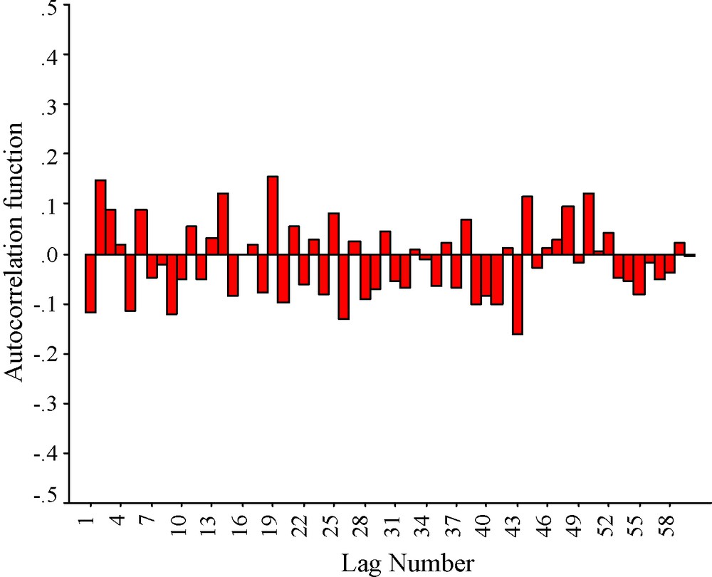
Autocorrelation function of the time series of the summer-monsoon rainfall amount over India.
Fonction d’autocorrélation des séries temporelles de quantité de pluie de mousson d’été sur l’Inde.
In the next step, it is examined whether there is any linear trend within the time series. A basic approach in testing for trends is the regression approach (Woodward and Gray, 1993, 1995). In the present problem, the months (t) constitute the independent variable and maximum temperature (Yt) the dependent variable. Thus, the model is Yt = a + bt + Et, where Et are the residuals, a is the regression constant, b is the regression parameter and t varies from 1 to 129. The estimates for b and a are given by
| (1) |
| (2) |
In the present paper, the values of the estimates for b and a are 0.0036 and 203.26. Under the assumption that the residuals are independent and normally distributed with zero mean, the estimated standard error for the estimate of b is (Woodward and Gray, 1993, 1995)
| (3) |
The null hypothesis of no linear trend is based on the assumption that is distributed as student's t with (n-2) degrees of freedom. In the present article, its value is 0.6922. Thus, the null hypothesis is accepted and it is concluded that there is no linear trend within the time series.
A time series can be modeled by an autoregressive [AR(p)], a moving average [MA(q)], an autoregressive moving average [ARMA(p,q)], or an ARIMA(p,d,q) model. The ARIMA, popularized by Box and Jenkins (1976), is used for describing a wide variety of time series behaviour. This model is either stationary or non-stationary in the boundary of the stationary region (Woodward and Gray, 1993). A detailed description of the ARIMA process and its theoretical background is available in (Box et al., 2007). An ARIMA(p,d,q) process is given by the equation (Box et al., 2007):
| (4) |
Here, B is the backward shift operator and
| (5) |
| (6) |
Some examples of application of ARIMA in the non-stationary meteorological time series include El-Fandy et al. (1994), Woodward and Gray (1993,1995) and Visser and Molenaar (1995). Three ARIMA(p,d,q) models namely ARIMA(0,1,1), ARIMA(0,2,2) and ARIMA(1,1,1) are now developed. Outcomes of the models are judged statistically. The three ARIMA models can be presented as:
ARIMA(0,1,1) process
| (7) |
ARIMA(0,2,2) process
| (8) |
ARIMA(1,1,1) process
| (9) |
Since the time series under consideration does not have any seasonal pattern, it is not required to take p,d and q greater than 2. The results will be discussed in subsequent sections.
2.2 Generation of autoregressive neural network
In the last section of the present paper, the non-linearity and non-stationarity of the time series have been established and non-stationary time series models have been generated. In the present section, ANN would be adopted to model the same time series. The ANN has been generated in autoregressive manner and consequently the model has been named as autoregressive neural network (ARNN) model. An ordinary autoregressive model of order p is written as
| (10) |
In Eq. (10), a linear function FL can be introduced, in which case the equivalent form of (10) would be (Dorffner, 1996)
| (11) |
Replacing L by an ANN model leads to the ARNN model. A few examples of ARNN studies include Temizel and Caset (2005), Sallehuddin et al. (2007) and Trapletti et al. (2000). An ARNN application to the modeling of geophysical time series is available in Chattopadhyay and Chattopadhyay (2009). The ARNN model can be written as (Dorffner, 1996)
| (12) |
At this juncture, it is necessary to decide the number of predictors in the ARNN model. This is done by fitting autoregressive (AR(p)) models to the time series. Testing AR models for p equals 1, 2, 3 and 4 and computing the Akaike's information criterion (AIC) statistics for all the time models the AR(4) model is identified as the best and consequently four predictors are used to generate the ARNN model. It should be noted that AIC is a screening statistic whose minimization implies best predictive model. The AIC is given by (Storch and Zwiers, 1999)
| (13) |
Details of the symbols used in the above expression are given in page 167, of Storch and Zwiers (1999). The neural network model adopted here belongs to the category of multilayer perceptron (MLP) (Gardner and Dorling, 1998 ; Gardner and Dorling, 1999). The theoretical details of MLP are available in various texts on ANN (e.g. Rojas, 1996 and Pal and Mitra, 1999); its suitability in hydrological modelling is well established in literature (Chattopadhyay and Chattopadhyay (2008a, 2008b) and references therein). Maier and Dandy (2000) presented an extensive review of the application of ANN in predicting water resource variables. In MLP, each network consists of several simple processors called neurons, or cells, which are highly interconnected and arranged in several layers. There are three basic types of layers: input layer, hidden layer(s) and output layer. Input and output layers are connected through hidden layer(s). There may be one to several hidden layers in between input and output layer. In mathematical form, the adaptive procedure of a feed forward MLP can be presented as
| (14) |
| (15) |
The above equation represents an iteration process that finds the optimal weight vector by adapting the initial weight vector w0. This adaptation is performed by sequential introduction of a set of input and target vectors to the network. The positive constant η is called the learning rate. The direction vector dk is the negative gradient of the output error function E.
In the present problem, the dataset (i.e. the time series) consists of 129 data points. Since there are four predictors in autoregressive manner, the proposed model can be written as:
| (16) |
In this model, the neural network is trained through Kalman Filtering with sigmoid non-linearity in both hidden and output layer. From the entire dataset, 70% of the data are chosen randomly to train the ARNN and the remaining 30% are chosen as the test data. The entire dataset is used as the validation set. The minimization of the root mean squared error is chosen as the stopping criterion. Genetic Algorithm trains the network through extensive variable selection. The maximum number of hidden nodes is chosen as 24 using the method proposed by Perez et al. (2000). After training through extensive variable selection, the final architecture (i.e. input nodes–hidden nodes–output node) combination comes out to be 3-3-1. Performance of the model would be discussed statically in the subsequent section.
3 Discussion
The first part of the discussion is to present a scatter plots for the (actual-predicted) pairs pertaining to all of the five models. In Fig. 2a, the scatter plot for ARIMA(0,1,1) shows that there is a negative association between actual and predicted rainfall. A linear regression line has been fit to the plot and it is seen that there is a tendency towards linearity but there are significant deviations from the linear regression line. The Fig. 2b, which corresponds to ARIMA(0,2,2) model, shows a good positive linear association between actual and predicted values and the regression line has a significant closeness with the data cloud. This indicates the presence of a good positive correlation between actual and predicted values. Fig. 2c, which corresponds to ARIMA(1,1,1), has a widely spread data points having little closeness to the linear regression fit. Thus, it is apparently felt that ARIMA(1,1,1) has less ability than ARIMA(0,1,1) and ARIMA(0,2,2) to represent the time series under consideration. The Pearson correlation coefficients are calculated for each of the three cases and Table 1 shows that ARIMA(0,2,2) has the largest positive correlation; ARIMA(0,1,1) has negative correlation which is less in magnitude than the ARIMA(0,2,2); ARIMA(1,1,1) has very small positive correlation. Thus, from the figures and the correlation values, the third ARIMA model seems to have the least prediction capability. Willmott (1982) raised some vital questions regarding the usefulness of Pearson correlation coefficients and the scatter plots as measures of goodness of fit of a model. According to Willmott (1982), the main problem associated with the Pearson correlation coefficients is that the magnitudes of such correlations are not consistently related to the accuracy of prediction, where accuracy is defined as the degree to which model-predicted observations approach the magnitudes of their observed counterparts. Willmott (1982) proposed an ‘index of agreement’ d as a measure of goodness of fit of a model to the observed data. This index is given by
| (17) |
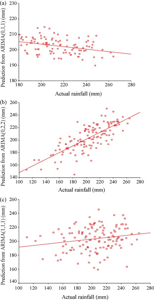
Scatter plots showing the association between actual summer monsoon rainfall and predictions from ARIMA(0,1,1) (a), ARIMA(0,2,2) (b) and ARIMA(1,1,1) (c).
Diagramme de dispersion des points montrant l’association des points entre pluie de mousson d’été actuelle et prédictions à partir d’ARIMA (0,1,1) (a), ARIMA(0,2,2) (b) et ARIMA (1,1,1) (c).
Mesures des indices de Willmott et corrélation de Pearson pour les modèles étudiés.
| Statistics | ARIMA(0,1,1) | ARIMA(0,2,2) | ARIMA(1,1,1) | ARNN |
| Willmott's index | 0.972 | 0.815 | 0.837 | 0.990 |
| Pearson correlation | −0.427 | 0.766 | 0.196 | 0.987 |
Here, Pi and Oi denote the predicted and actual values of the ith observation of the time series. The values of the said statistic for the three models are presented in Table 1. It is observed from Table 1 that ARIMA(0,1,1) produces the maximum values of d. This means that the ARIMA(0,1,1) fits the best to the monsoon rainfall time series under consideration. As a further support to this observation, the Akaike Information Criteria (AIC) are calculated for the three models. It is found that the ARIMA(0,1,1) produces minimum AIC (1228.99), whereas, ARIMA(0,2,2) and ARIMA(1,1,1) produce AIC of 1256.96 and 1243.78 respectively. Since the minimization of AIC indicates better model, goodness of ARIMA(0,1,1) over the other models is further supported. The Pearson correlation and Willmott's index are calculated also for the ARNN model. It is found that the values are 0.987 and 0.99 respectively (Table 1). Thus, it is understood that ARNN outperforms ARIMA(0,1,1), which produced the maximum Willmott's index of agreement (0.972) among the competitive ARIMA models. However, ARIMA(0,1,1) can be considered as an alternative to ARNN because of its high Willmott's index, which is a little distant from that produced by ARNN model. A scatter plot is presented in Fig. 3, which corresponds to the actual versus predicted monsoon rainfall for the ARNN model. A very prominent positive and linear association is discernible from this figure. The data points are so close to the regression line that in some cases it seem that they are almost coincident with the regression line. To make the presentation more understandable, we have prepared a line diagram in Fig. 4, which shows that the actual and predicted summer monsoon rainfall amounts are very close to each other in the case of ARNN.
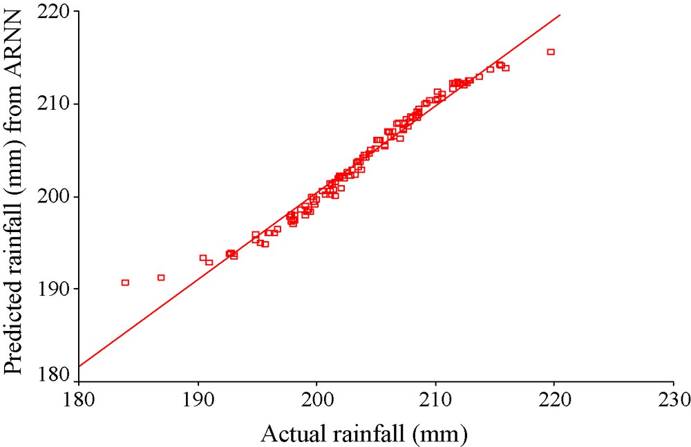
Scatter plots showing the positive linear association between actual summer monsoon rainfall and predictions from autoregressive neural network (ARNN) model.
Diagramme de dispersion des points montrant l’association positive linéaire entre pluie de mousson d’été actuelle et prédiction à partir du modèle autorégressif à réseau neuronal (ARNN).
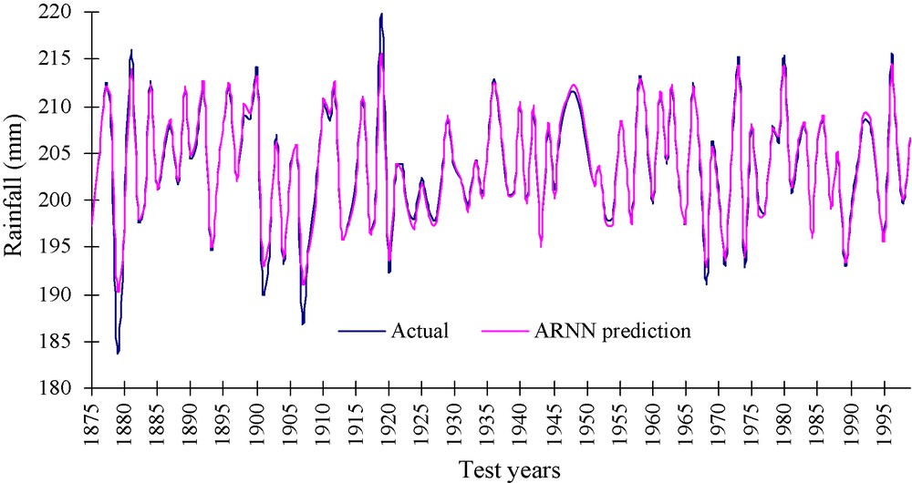
Line diagram showing the association between actual summer monsoon rainfall and predictions from autoregressive neural network (ARNN) model.
Diagramme linéaire montrant l’association entre pluie de mousson d’été actuelle et prédictions à partir du modèle autorégressif à réseau neuronal (ARNN).
4 Concluding remarks
The present article has aimed at developing a univariate model for the monsoon rainfall time series over India. Rainfall is an essential component of the hydrological cycle and the monsoon season (June–August) of India is the most productive period for agricultural practices in this country. In some parts of this country, the monsoon rainfall is stored for future cultivation purposes. Several multivariate models have been attempted for the said time series. However, univariate modelling is not very frequent in this field. Authors of the present paper felt that a univariate model might be of more importance for predicting the said time series because it would not require the data for any other meteorological parameters. It was also felt that a univariate approach would be more acceptable in areas where some decisions need to be taken in light of the limited data availability. Prior to generating the representative models for the said time series, the serial correlation pattern of the time series was studied and the absence of any persistence within the time series was revealed. Simultaneously, absence of any cyclic pattern was also perceptible. From this study, it could be understood that the time series was not characterized by any stationarity. Instead, the time series was characterized by randomness. The presence of any linear trend within the time series was also investigated and it was detected that there was no linear trend within the time series. Subsequently, a non-linear time series approach in the form of ARIMA has been generated for the time series. After judging the three ARIMA models statistically, the ARIMA(0,1,1) was identified as the best model. Finally, an ARNN model was generated, where the number of predictors was decided on the basis of an autoregressive approach. Four predictors were required for the ARNN modelling, where the neural network was trained as multilayer perceptron with sigmoid non-linearity. After training through extensive variable selection by genetic algorithm, it was revealed that three nodes in the hidden layer with three nodes in input layer of the final model would be the best network architecture. Performance of the ARNN was judged statistically by means of scatter plot presentation and Willmott's index computation and it was revealed that the ARNN model performed better than ARIMA(0,1,1). However, from the high value of Willmott's index, it could be said that ARIMA(0,1,1) was not a negligible model and it might be an alternative model for forecasting the monsoon rainfall time series over India if there were no scope for neural network modelling.