

1 Introduction
Since folded structures have been discovered and described in Wales and in the Alps in the late 1700s, the understanding of their origin and structure has become one of the main problems of structural geology. After a period of speculative hypotheses based on the evolution of tectonic structures, the plate tectonics theory has been formulated to account for most geological problems. Development of tectonophysics during second half of the XXth century has brought new methods and results, i.e., analogue and numerical modelling, analyses of stress-state from fractures for paleostructures (Angelier, 1984; Goustchenko, 1975; Gzovsky, 1954) and earthquake focal mechanisms for recent structures (Brune, 1968; Goushtchenko, 1996; Kostrov, 1968; Rebetsky, 1996; Yunga, 1979). Significant efforts were spent to determine the strain at the specimen scale; corresponding methods are intensively developed now (Erslev and Ge, 1990; Fry, 1979; Lisle, 1985; Ramsay, 1967). Large volumes of high quality materials related to the structure and strain of foreland zones have been obtained using the method of balanced cross-sections (Dahlstrom, 1969; Hossak, 1979). However, until now there is no commonly accepted method to study structure and the formation mechanism of hinterland multi-scale objects. Of course, it is possible to find interpretative models (see Dotduev (1997), Robinson et al. (1996) for the Greater Caucasus), but they are not based on the results of detailed tectonophysics analysis. Therefore the reliability of such models is disputable.
The most difficult task remains to define the shortening value. Methods of strain analysis are applied to local structures only. Attempts to integrate results of many measurements even within the same fold meet problems. It is well known that balanced cross-sections cannot be used for small folds in the hinterland. Assessment of shortening based on paleomagnetic data and on the tectonic approach of sedimentary facies is too rough to give accurate values. Some recent studies have been devoted to the determination of shortening in folds based on the shape of layers (for example, Schmalholz and Podladchikov (2001), Srivastava and Shah (2008)). However, for different reasons these methods have only limited applicability. The review of information, which can be obtained from folds for an estimation of strain value, rheology and of other prominent aspects of formation of single-layered and multilayered systems can be found in Hudleston and Treagus (2010). Altogether, this means that the structural basis of modern geodynamic models is not reliable. At the same time it is clear that each fold is a source of detailed information on strain value and development mechanisms.
2 Basic approach
This article presents a review of the long-term efforts and results of studies of linear fold kinematics, initiated by Pr Vladimir Beloussov (who was born in 1907, and died in 1990). These methods are based on the kinematic mechanisms of structure formation at different scales, from individual grains up to the scale of the entire fold belt system. The set of these methods is called multi-rank strain analysis (Yakovlev, 2008a). The models link the geometry of natural objects to variation laws of an object's geometry, including its formation mechanisms and value of strain. Obviously, having the possibility to distinguish among various mechanisms and measuring geometric parameters, we can define the value of spatial shortening. It is important that a solution is searched from small structures to large ones, at any scale and without omissions. The final result is the reconstructed geometry of large structures, which is independent from any geodynamic concept. Within the hierarchic system of objects, several levels are recognized (Rebetsky et al., 2004), which differ by their number of layers.
Level 1: intralayer strain of grains and inclusions; 2: separate folds (layer and pairs of competent and incompetent layers); 3: domains (package of layers, see example on Fig. 1C); 4: structural cells (term by Goncharov (1988)) or tectonic modules; 5: tectonic zone; 6: folded system (such as the Greater Caucasus); 7: the whole folded thrust belt. In this hierarchic system (Rebetsky et al., 2004), the sedimentary cover is usually at level 4, crust at level 5, and the whole lithosphere at the highest level 7.
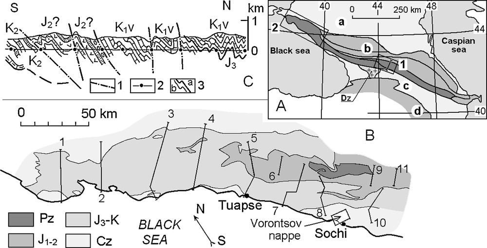
Locations of the study areas. A. Locations of the Chiauri tectonic zone (1) and North-West Caucasus (2) within the overall structure of Greater Caucasus; a: Scythian plate; b: Greater Caucasus, including main tectonic zones; c: Trans-Caucasus massif, Dzirulsky crystalline block (Dz) is shown as part of the massif; d: Lesser Caucasus structures. B. Sketch geological map of North-West Caucasus; positions of structural sections (Giorgobiani and Zakaraya, 1989; Sholpo et al., 1993) and of the Vorontsov nappe are indicated. C. Middle part of section No. 8 (Sholpo et al., 1993) is shown as example of data used for study. Ages of deposits: J2, J3 is Middle and Upper Jurassic, K1v is Valanginian, K2 is Upper Cretaceous; 1: faults plains, 2: boundaries of domains on section line, 3: boundaries of stratigraphic units (a) and layers (b). Masquer
Locations of the study areas. A. Locations of the Chiauri tectonic zone (1) and North-West Caucasus (2) within the overall structure of Greater Caucasus; a: Scythian plate; b: Greater Caucasus, including main tectonic zones; c: Trans-Caucasus massif, Dzirulsky crystalline block (Dz) ... Lire la suite
Localisation des régions étudiées : A. Localisation de la zone tectonique de Chiauri (1) et du Caucase nord-occidental (2) dans la structure du grand Caucase ; a : plaque scythienne ; b : carte montrant les principales zones tectoniques du Grand Caucase ; c :massif trans-caucasien, le bloc cristallin de Dzirulsky (Dz) étant montré comme une partie du massif ; d :structures du Petit Caucase. B. Carte géologique schématique du Caucase nord-occidental ; les positions des coupes structurales (Giorgobiani et Zakaraya, 1989 ; Sholpo et al., 1993) et de la nappe de Vorontsov sont indiquées. C. La partie moyenne de la section no 8 (Sholpo et al., 1993) est présentée comme exemple de données utilisées pour l’étude ; âges des dépôts : J2 et J3 correspondent au Jurassique moyen et supérieur, K1v au Valanginien, K2 au Crétacé supérieur ; 1 : plan de faille, 2 : limite des domaines sur la ligne de section, 3 : limites des unités (a) et des couches (b) stratigraphiques. Masquer
Localisation des régions étudiées : A. Localisation de la zone tectonique de Chiauri (1) et du Caucase nord-occidental (2) dans la structure du grand Caucase ; a : plaque scythienne ; b : carte montrant les principales zones tectoniques du Grand Caucase ; c :massif trans-caucasien, le bloc ... Lire la suite
Boundaries between objects in the hierarchic system are given in such way that it remains coherent within the limits of acting mechanisms. The relationships between the different hierarchic levels will be given in the article for different scales, using a wide range of structures from the Greater Caucasus example (Fig. 1).
3 Buckling models applied to single folds
Single folds are recognized at level 2 of the hierarchic system. They occur both at small and large scales. Two mechanical models are used to determine the value of shortening within a single fold:
- • from a mechanics point of view, folding of single viscous layers incorporated in a less viscous environment has a clear theory of formation, which is used for computation within the finite-element model (Hudleston and Stephansson, 1973). This model predicts the whole geometry of the fold and makes it possible to construct a diagram, linking geometric parameters to the amount of shortening during the process (Yakovlev, 1978, 2008b). Measuring the same parameters in a natural structure (Fig. 2) allows one to define the value of shortening and to derive the viscosity contrast from the diagrams. Application of the method to 78 structures of the Chiauri zone in the Greater Caucasus gave 56% of average shortening (−ɛ = (L1−L0) × 100/L0) with data scattering from 25 to 82%;
- • for multilayer folds a kinematic iterative model of shape transformation was built. This model combines buckling and flattening for the competent layers and shearing with rotation and flattening for adjacent incompetent layers. Based on this model, inclination of the layers in the flanks and ratio of competent layer thickness between the flanks and hinge of a given fold allow one to estimate the shortening in the direction perpendicular to the axial plane (Yakovlev, 2002). Application of the iterative model to 36 folds of the Chiauri zone gave results (average shortening 57%, scatter from 27 to 83%) similar to those obtained from the modeling of single layers observed in the same area. For 8 local structures the two types of folds were found, which makes it possible to compare results of the two methods. The comparison demonstrates that the kinematic model of multilayers folds is, in general, close to the model of formation of single viscous layer folds.

Method for analysing single viscous layer folds. A. Diagram for the measurement of shortening value (-ɛ, SH) and viscosity contrast (VC). Ordinate axis (Y) is interlimb angle (α), abscissa axis (X) is ratio length/thickness (L/T) (after Yakovlev (1978)). B. Scheme of measurements of interlimb angle (α, between lines which connected top and bottom of layer in adjacent hinges), length of flanks (L, distance between top of layer in anticline and bottom in syncline) and layer thickness (T, in hinge) in models and natural folds. The model shown is for a viscosity contrast of 100 (Hudleston and Stephansson, 1973). C. Scheme of measurements of geometric parameters in natural folds. D. Histogram for VC parameter for 73 folds trains (X axis is “viscous contrast”, Y axis is frequency). E. Histogram for SH parameter (X axis is “shortening value, %”, Y axis is frequency). For A: 1: sub-vertical isolines, after model parameters and interpolated isolines, outlining the viscosity contrast value VC; 2: sub-horizontal isolines, outlining the shortening value Sh; 3: points plotted after measurements for 5 folds in natural series of folds (C) and averaged values point (circle). Masquer
Method for analysing single viscous layer folds. A. Diagram for the measurement of shortening value (-ɛ, SH) and viscosity contrast (VC). Ordinate axis (Y) is interlimb angle (α), abscissa axis (X) is ratio length/thickness (L/T) (after Lire la suite
Méthodes pour l’analyse de plis simples à couches visqueuses. A. Diagramme pour la mesure de la valeur de raccourcissement (-epsilon, SH) et contraste de viscosité (VC). Sur l’axe des ordonnées (Y), angle alpha entre les flancs des plis, sur l’axe des abscisses (X), rapport longueur/épaisseur (L/T) (d’après Yakovlev (1978)). B. Schéma de mesure de l’angle entre les flancs (alpha souligné entre les lignes qui relient le sommet et la base de la couche dans des charnières adjacentes), longueur des flancs (L, distance entre le sommet de couche dans l’anticlinal et la base dans le synclinal), épaisseur de la couche (T, dans la charnière), dans les modèles et les plis naturels. Le modèle présenté correspond à un contraste de viscosité de 100 (Hudleston et Stephansson, 1973). C. Schéma de mesure des paramètres géométriques dans des plis naturels. D. Histogramme pour le paramètre VC dans le cas de 73 trains de plis (sur l’axe X, « contraste visqueux », sur l’axe Y, fréquence). E. Histogramme pour le paramètre SH (sur l’axe X, valeur du raccourcissement en pourcent, sur l’axe Y, fréquence). Pour A : 1 : isolignes sub-verticales d’après les paramètres du modèle et isolignes interpolées soulignant la valeur du contraste de viscosité ; 2 : isolignes sub-horizontales soulignant la valeur du raccourcissement Sh ; 3 : points représentatifs, après mesure de 5 plis d’une série naturelle de plis (C) et un point de valeur moyenne (cercle). Masquer
Méthodes pour l’analyse de plis simples à couches visqueuses. A. Diagramme pour la mesure de la valeur de raccourcissement (-epsilon, SH) et contraste de viscosité (VC). Sur l’axe des ordonnées (Y), angle alpha entre les flancs des plis, sur ... Lire la suite
Multilayers folds were found in the Sochi region in the North-West Caucasus in the footwall of the Vorontsov nappe (Yakovlev et al., 2007, 2008) near the foreland/hinterland boundary (location on Fig. 1B). Two possible deformation models of the structure were tested, corresponding to different geodynamic situations: pure shear (Ramsay and Huber, 1987) with an horizontal shortening linked to the Greater Caucasus development and simple shearing along the sole of the nappe. Two parameters, i.e., the inclination of folds axial plane and the value of shortening perpendicular to the axial plane, have shown significantly different trends of development within the two models (Fig. 3).
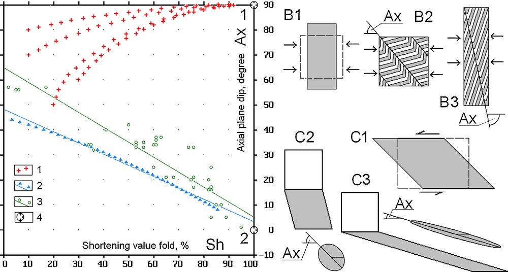
Study on the origin of the Vorontsov nappe. A. Comparison diagram of 2 models and kinematic parameters for natural fold data (Yakovlev et al., 2008). B1–B3 document the lateral shortening model. C1–C3 document horizontal shear model. For A: 1: trends for 4 sites accounting for the lateral shortening model; 2: trend and regression line for the horizontal shear model; 3: folds data and regression line for natural fold parameters; 4: extreme value for lateral shortening models (1) and for horizontal shear model (2). B1: kinematic model for lateral shortening; B2: initial state; B3: more advanced stage of shortening; Ax: axial fold plane dip is increasing from B2 to B3 (Sh - shortening value is increasing also). C1: kinematic model of horizontal shearing; C2 and C3 display the initial and more advanced deformation stages, folds axial plane dip (Ax) is decreasing, but shortening value is increasing during incremental deformation. Masquer
Study on the origin of the Vorontsov nappe. A. Comparison diagram of 2 models and kinematic parameters for natural fold data (Yakovlev et al., 2008). B1–B3 document the lateral shortening model. C1–C3 document horizontal shear model. For A: 1: trends ... Lire la suite
Étude de l’origine de la nappe de Vorontsov. A. Diagramme comparatif de 2 modèles et paramètres cinématiques à partir de données sur des plis naturels (Yakovlev et al., 2008). B1–B3 représentent le modèle de raccourcissement latéral. C1–C3 représentent le modèle de cisaillement horizontal. Pour A : 1 : tendances pour 4 sites rendant compte du modèle de raccourcissement latéral ; 2 : lignes de tendance et de régression pour le modèle de raccourcissement horizontal ; 3 : données relatives aux plis et ligne de régression pour les paramètres de plis naturels ; 4 : valeurs extrêmes pour les modèles de raccourcissement latéral (1) et de cisaillement horizontal (2). B1 : modèle cinématique de raccourcissement latéral ; B2 : stade initial ; B3 : stade plus avancé de raccourcissement ; Ax : pendage du plan axial du pli, augmentant de B2 à B3 (Sh, valeur du raccourcissement, augmente aussi). C1 : modèle cinématique de cisaillement horizontal ; C2 et C3 présentent les stades de déformations initiales et plus avancées, le pendage du plan axial des plis (Ax) est décroissant, mais la valeur du raccourcissement est croissante pendant l’incrément de déformation. Masquer
Étude de l’origine de la nappe de Vorontsov. A. Diagramme comparatif de 2 modèles et paramètres cinématiques à partir de données sur des plis naturels (Yakovlev et al., 2008). B1–B3 représentent le modèle de raccourcissement latéral. C1–C3 représentent le modèle de cisaillement horizontal. ... Lire la suite
These parameters were measured in 39 folds of the Vorontsov nappe and are close to the simple shear model prediction. A difference in 20 degrees between regression lines could be explained by the nappe body dipping 20 degrees to the north at the measurement spot. The initial general dip should have been to the south, which would agree with a gravitational origin for the nappe emplacement. Additional detailed analysis of sedimentary sequences in adjacent tectonic zones and the analysis of the geological map of the Caucasus have revealed the following sequences for the major tectonics events in this region: (1) main folding inside the nappe itself occurred 35–25 Ma ago; (2) southward gravitational sliding of the nappe toward the basin over gently dipping submarine relief took place 22–15 Ma ago; (3) main uplift of the mountain range has started at 14 Ma (Yakovlev et al., 2008). This kinematic modeling at the hierarchic level 2 has proved that gravitational sliding is the most likely cause for the Vorontsov nappe formation, which is therefore not directly related to crustal shortening and mountain building processes. For this reason the 15 km long southward displacement of this 1.5-km thick plate should not be included in the overall shortening value of the Greater Caucasus, which must be deduced from higher hierarchic levels.
4 Description of strain for isometric volumes - folded domains
The hierarchic level 3 (Rebetsky et al., 2004) integrates several folds which have similar parameters in a unique domain: (1) axial plane dip; (2) value of shortening; and (3) local dip of the envelope of the small scale folds. It is important that characteristics of folds from a single layer in a limited volume can be extrapolated to a pack of layers (0.3–1.5 km thick), which make it possible to describe the strain of the whole volume using the concept of the strain ellipsoid (Fig. 4). The boundaries of individual tectonic domains are defined parallel to the axial plane of folds. These boundaries are located at the place where fold parameters change or where sharp changes of lithology occur. Fault plains are using as boundaries also, if significant displacement of blocks takes place.

Concept of strain ellipsoid in a fold and in a domain (after Yakovlev and Voitenko (2005)). A. Model of multilayer fold, outlining both the total strain ellipsoid and ellipses for individual layers. Ellipsoid axes: elongation. ɛ3 = l1/l0 = 2.13, ɛ2 = l1/l0 = 1.0, shortening ɛ1 = l1/l0 = 0.47. 1: axial plane of the fold; 2: hinge line; 3, 4: strain ellipses in a competent layer (3) and in an incompetent one (4). B. Domain parameters. 1: horizontal plane; 2: envelope surface and its dip angle En; 3: axial plane and its dip angle Ax; 4: strain ellipsoid, shortening value SH may be measured by interlimb angle φ; 5: domain part of section line, its length and dip angle. Masquer
Concept of strain ellipsoid in a fold and in a domain (after Yakovlev and Voitenko (2005)). A. Model of multilayer fold, outlining both the total strain ellipsoid and ellipses for individual layers. Ellipsoid axes: elongation. ɛ3 = l1/l0 = 2.13, ɛ2 = l1/Lire la suite
Concept d’ellipsoïde de déformation dans un pli et dans un domaine (d’après Yakovlev et Voitenko (2005)). A. Modèle de pli multicouche soulignant à la fois l’ellipsoïde de déformation totale et les ellipses pour chaque couche. Axes d’ellipsoïde : allongement ɛ3 = l1/l0 = 2,13, ɛ2 = l1/l0 = 1 ; raccourcissement ɛ1 = l1/l0 = 0,47. 1 : plan axial du pli ; 2 : ligne de charnière ; 3, 4 : ellipses de déformation dans un feuillet compétent (3) et incompétent (4). B. Paramètres de domaine. 1 : plan horizontal ; 2 : surface de l’enveloppe et son angle de pendage En ; 3 : plan axial et son angle de pendage Ax ; 4 : ellipsoïde de déformation, la valeur Sh de raccourcissement peut être mesurée par l’angle entre les flancs ; 5 : partie du domaine de la ligne de section, sa longueur et son angle de pendage. Masquer
Concept d’ellipsoïde de déformation dans un pli et dans un domaine (d’après Yakovlev et Voitenko (2005)). A. Modèle de pli multicouche soulignant à la fois l’ellipsoïde de déformation totale et les ellipses pour chaque couche. Axes d’ellipsoïde : allongement ɛ3 = l1/Lire la suite
This hierarchic level (Rebetsky et al., 2004) is a major one to incorporate the local scale natural observations (Fig. 1C) in the regional cross-sections crossing the tectonic zones. This work step is implicitly or explicitly used during any cross-section balancing procedure (Boyer and Elliott, 1982). The value of shortening of folds in individual tectonic modules should be taken from results of the methods described above. However, mostly this parameter is defined from the fold interlimb angle, an assumption also developed in the works (Suppe, 1983) on kink-bends folds and Ghassemi et al. (2010) for “similar folding”. When doing this it is assumed that layer length at flanks is constant, which is in general proved in studies of natural structures in the Caucasus at least. From the three above retained parameters, kinematical models were issued allowing the realization of diagnostic diagrams (Yakovlev, 2001).
For studying natural linear folding it is very important to have detailed structural cross-sections. The North-West Caucasus was studied in details by T. Giorgobiani and Y. Rogozhin (Giorgobiani and Zakaraya, 1989; Sholpo et al., 1993). Eleven cross-sections compiled by them served as the basis for several types of studies (Fig. 1B, C). In these cross-sections nearly 250 domains were defined. Three afore-mentioned geometrical parameters of the structures were measured (Fig. 4B), i.e., the dip angle of axial planes (AX), the dip of the envelope plane of the small scale folds (EN), and the value of fold shortening (SH). Using diagnostic diagrams that take into account the three measurements (Yakovlev, 2001), it was found that near-fault fold measurements make a specific cluster (Fig. 5B). Such a structure could be linked to a superposition of simple shearing along inclined zone and horizontal pure shear (Fig. 5C). Two kinematical models were compiled with different dips of the shear zone (45° and 20°) and different model increments concerning the amount of simple shear and pure shear. It was found that the best fit for the morphology of those local structures is obtained with a shear zone that initially dips at 45° and a succession of 6° shearing along the shear zone and 1% of horizontal pure shear (horizontal shortening) (Yakovlev, 2005). Distribution on a map of such structures with northern or southern vergence demonstrates regular features and gives a key for tectonic zoning of the region. This study implies that a study at hierarchic level 3 can provide a key to understanding the geodynamics at a higher hierarchic level. Small-scale folding is probably related to pairs of shear zones with standard shear angle, occurring under horizontal compression, rather than slip along tilted bedding (20° as initial tilt) or detachment operating at the top of the basement. It should be noted that the structures of high hierarchic level cannot be easily identified during geological mapping or as a result of structural section compilation.

Detecting forming mechanisms for inclined ductile shear zones. A. Scattering diagram in domain parameters EN and AX; gray sectors show the studied data sets; a, b, c: illustrations of domain morphology for three places on diagram; “vertical” section on line (AX-EN) is shown. 1: inclined zones domains with vergence to south; 2: the same to north; 3: other domains with some basic mechanisms. B. Scattering diagram for studied domains in parameters (AX-EN) and SH; a, b: illustrations of domains morphology; 1: domains with Northward vergence; 2: averaged points, forming the main trend; 3: domains with Southward vergence. C. Scheme of mechanisms model; a: initial stage; b: final stage. D. Diagrams for comparison natural data trend and two models trends. D1: model with initial dip of shearing zone 45°; D2: with initial dip 20°; 1: started point, a: final point for best trend of model; b: final point for natural data trend. Several versions of models with increments of shortening and shearing are shown. Version dip 45° and increments 1% – 6° is best. Masquer
Detecting forming mechanisms for inclined ductile shear zones. A. Scattering diagram in domain parameters EN and AX; gray sectors show the studied data sets; a, b, c: illustrations of domain morphology for three places on diagram; “vertical” section on ... Lire la suite
Détection des mécanismes de formation des zones de cisaillement ductile inclinées. A. Diagramme de dispersion des paramètres des domaines EN et AX ; les secteurs gris indiquent les groupes de données ; a, b, c : illustrations de morphologies de domaines pour trois zones sur le diagramme ; section verticale sur la ligne (AX – EN). 1 : domaines de zones inclinées avec vergence vers le sud ; 2 : la même chose vers le nord ; 3 : autres domaines avec quelques mécanismes de base. B. Diagramme de dispersion dans les domaines étudiés pour les paramètres (AX – EN) et SH ; a, b : illustrations de morphologies de domaines ; 1 : domaines à vergence vers le nord ; 2 : points moyens constituant la tendance principale ; 3 : domaines à vergence vers le sud. C. Schéma du modèle des mécanismes ; a : stade initial ; b : stade final. D. Diagrammes comparatifs de la tendance indiquée par les données de la nature et celles indiquées par les deux modèles. D1 : modèle avec pendage initial de la zone de cisaillement à 45° ; D2 : avec pendage initial de 20°, 1 : point de départ, a : point final pour la meilleure tendance du modèle, b : point final pour la tendance des données naturelles. Différentes versions de modèles avec augmentation de raccourcissement et de cisaillement sont présentées. La version avec pendage à 45° et incréments de 1 % – 6° est la meilleure. Masquer
Détection des mécanismes de formation des zones de cisaillement ductile inclinées. A. Diagramme de dispersion des paramètres des domaines EN et AX ; les secteurs gris indiquent les groupes de données ; a, b, c : illustrations de morphologies de domaines pour ... Lire la suite
The description of finite deformation in individual tectonic domains by a strain ellipsoid makes it possible to reconstruct the initial position of a single domain and of the whole cross-section (Yakovlev, 2002, 2009). To achieve this, we add to three measured geometrical parameters the next two parameters (Fig. 4B), i.e., (4) the length of the domain section line; and (5) the dip of section line. By so doing, the final state of the domain can be described as a strain ellipsoid (aliquot ellipse for 2D linear folding), the orientation of which is constrained by the initial geometry of the layers. Its volume is limited horizontally by a specific segment of the profile, which is characterized by a given length and a given dip.
The main problem to reconstruct the pre-folded state of a given domain relates to the selection of the backward kinematic operations, which will bring the fold architecture back to horizontal layers and the aliquot ellipse back to a circle. We have used 3 distinct operations: (a) a rotation back up to the horizontal position of the fold envelope plane; (b) a horizontal shearing to restore the fold axial planes back to a vertical position; and (c) a horizontal extension up to fold straightening, when the ellipse will turn back into a circle. During these operations both the length and the orientation of the profile segment are changed. For instance, in the pre-folded state, this line will have a new length and a new inclination relative to the horizontal layering (Fig. 6). It is known (Ramsay and Huber, 1987) that the order of the three operations will influence the result. However, the same result of reconstruction can be obtained with another order of operations. For instance, we can operate first the rotation back up to obtain a vertical position of the axial plane, followed by a vertical simple shearing up to horizontal position of envelope plane and finally a stretching; but, of course, other parametric values should then be used for these operations.
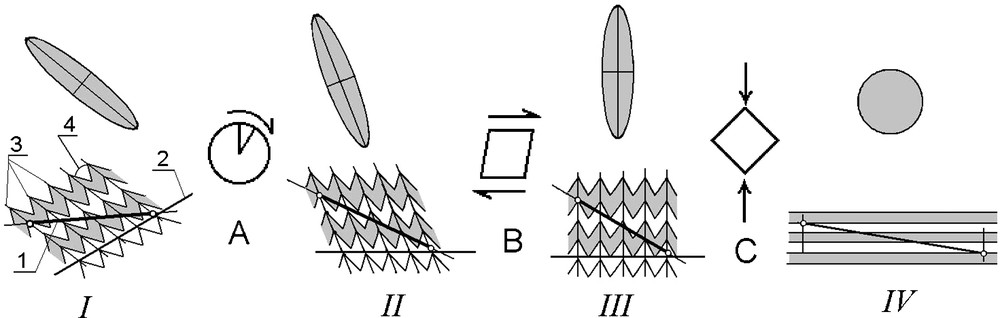
Operations for restoration of domain pre-folded state (IV) from recent state (I) (Yakovlev, 2009). Operations: A: rotation on angle of envelope plain dip (from I to II), B: horizontal simple shearing (II–III), C: horizontal elongation (III–IV). Perturbations of strain ellipse are shown. Symbolic folded structure is shown. 1: length and tilting of section line; 2: envelope plain dip; 3: axial plain dip; 4: interlimb angle as fold shortening value parameter.
Opérations pour la reconstitution d’un stade pré-plissé (IV) du domaine à partir d’un stade récent (I) (Yakovlev, 2009). Opérations : A : rotation sur l’angle de pendage de l’enveloppe du pli (de I à III) ; B : simple cisaillement horizontal (II–III) ; C : allongement horizontal (III–IV). Les perturbations des ellipses de déformation sont présentées, de même qu’une structure plissée symbolique. 1 : longueur et basculement de la ligne de section ; 2 : pendage de l’enveloppe ; 3 : pendage de l’axe ; angle entre les flancs en tant que paramètre valeur de raccourcissement de pli. Masquer
Opérations pour la reconstitution d’un stade pré-plissé (IV) du domaine à partir d’un stade récent (I) (Yakovlev, 2009). Opérations : A : rotation sur l’angle de pendage de l’enveloppe du pli (de I à III) ; B : simple cisaillement horizontal (II–III) ; ... Lire la suite
Another very important parameter is the “initial depth”, that is, the location of the tectonic domain in the stratigraphic column. Each domain extends between two initial depths along the stratigraphic column. Fault surfaces are considered as planes belonging to one of the domains and initial pre-folded orientation of this plane is calculated using the same sequence of the three basic kinematic operations. Then, the “initial depth” difference between two adjacent blocks will define the amplitude of the vertical offset whereas the inclination angle of the plane in its pre-folded state will define the amplitude of the horizontal displacement. A full restoration of the pre-folded state of the whole cross-section is then possible by merging the un-folded states of individual domains and displacing them along the faults.
5 Complete restoration of the geometry of sedimentary cover structures
The basic concept here is similar to the goals of the balanced cross-section procedure (Dahlstrom, 1969), but we propose a systematic procedure to incorporate the data from one hierarchic level to the other. Furthermore, we would like to outline on the following modelling example that restoration of the geometry of sedimentary cover structures is not restricted to line length balancing methods. It requires also involving the deformation obtained at a smaller hierarchic level and to assess correctly the tectonic (external) component of the shortening.
At the scale of a structural cell (hierarchical level 4) Goncharov (1988) developed a pure kinematic model for calculations of field displacement within a convective structural cell based on hydrodynamic equations. Such a model makes it possible to calculate strains (strain ellipses) for small volumes (domain, hierarchical level 3) from the intensity of convection and of the external shortening of the whole structural cell. This study makes it possible also to model kinematically the combination of folding of the sedimentary cover together with internal deformation within individual domains, and to solve a problem which does not have analytical solution in mechanics (Fig. 7). In particular, we can get a model for quasi-buckling at the scale of the sedimentary cover by calculating the combination of parameters which keep constant the whole length of the central layer of the structural cell (la-lb-lc on Fig. 7). If we trace the changes of the length of segments formed by several domains (such segments not being located this time in the middle of the structural cell), their shortening values will strongly differ from each other. Therefore, if we want to evaluate tectonic shortening within complex folded structure, we have to study the structural location of the structural cells in order to integrate the shortening of these objects in the whole structure.

Structural cell as the minimal structure in which a horizontal shortening value is coinciding with tectonic related shortening at scale of the whole sedimentary cover (Yakovlev (2008a), with changes). A. Two adjacent cells in initial state (L0). B. The same two cells after buckling (L1), explanation in text. Shortening value of cell L1/L0 = 0.87. 1: initial net (a) and its modifications (b, constant length line la-lb-lc); 2: symbolic folds in domain; 3: segments of structure; 4: value of shortening for segment. Masquer
Structural cell as the minimal structure in which a horizontal shortening value is coinciding with tectonic related shortening at scale of the whole sedimentary cover (Yakovlev (2008a), with changes). A. Two adjacent cells in initial state (L0). B. The same ... Lire la suite
Module structural en tant que structure minimale, dans laquelle la valeur du raccourcissement horizontal coïncide avec le raccourcissement lié à la tectonique, à l’échelle de l’ensemble de la couverture sédimentaire (Yakovlev (2008a), modifié). A. Deux cellules adjacentes au stade initial (L0). B. Les deux mêmes cellules après action de quasi –flexion (Ll), explication dans le texte. Valeur du raccourcissement de cellule L1/L0 = 0,87. 1 : réseau initial (a) et ses modifications, (b, ligne de constante longueur la-lb-lc) ; 2 : plis symboliques du domaine ; 3 : segment de structure ; 4 : valeur du raccourcissement pour le segment. Masquer
Module structural en tant que structure minimale, dans laquelle la valeur du raccourcissement horizontal coïncide avec le raccourcissement lié à la tectonique, à l’échelle de l’ensemble de la couverture sédimentaire (Yakovlev (2008a), modifié). A. Deux cellules adjacentes au stade initial ... Lire la suite
Information on thickness of the cover together with data on pre-folded length of all domains makes it possible to define the initial geometry of these structural cells. Both the pre-folded state coordinates of structural cells boundaries and the initial thickness of sedimentary cover are required to build series of 2D restored profiles.
For the example of the North-West Caucasus region, data on the thickness of all stratigraphic horizons from the Lower Jurassic to the Upper Eocene were collected for the 244 tectonic domains of the 11 cross-sections (Fig. 1B). This allows one to reconstitute the whole sedimentary cover. Interpolation between the entire set of cross-sections provided a 3D description of the architecture of the sedimentary cover of the North-West Caucasus.
Another important problem relates to the onset and duration of the folding process and its relation to the mountain building process for the Greater Caucasus, the precise timing of which is still being debated. The general reviews of the information on the whole structure of the Greater Caucasus can be found in Leonov (2007), and Saintot et al. (2006). It is often considered that the main folding episode occurred before or during the Oligocene and that mountain topography has started to be formed during the Sarmatian. According to the age of angular unconformities on the edges of the Greater Caucasus and by the age of the first conglomerates, these two processes may be indeed diachronous. The lack of refolding of erosional surfaces confirms this idea (Nesmeyanov, 1992). However, there is more information, which demonstrates the long duration of folding formation and its simultaneity with the relief formation at least in a few local structures.
To restore the former architecture of the Greater Caucasus, it is necessary to have some ideas about its tectonic evolution. As a first hypothesis, we have considered here three successive evolutionary stages: Stage 1 is characterized by the end of the deposition of Pre-Oligocene series; during stage 2, still before the Sarmatian, the whole folded structure is formed without any erosion, whereas these folded structures became subsequently eroded during mountain growth processes. Accordingly, stage 3 relates to the modern post-orogenic structure. At present it is not possible to calculate the amount of erosion, which could have operated during the Oligocene episode of folding or later, nor to offer more precise model based on it. In this context, the second stage is rather artificial and is mainly used for the purpose of numeric simulations.
The main parameters for the restoration are deduced from the analysis of the cross-sections. They comprise the pre-folded length of sections, ranging from 40–50 to 70–80 km, as well as the initial thickness of the sedimentary cover, ranging from 7 to 17 km, with a mean value of 13 km. Only 3 to 5 structural cells are sufficient to describe the Greater Caucasus during its first stage of evolution. Depths of the basement top for the second evolutionary stage (folding stage) of the model were calculated from value of shortening and structural (post-folded) thickness of the sedimentary columns for 42 structural cells (definitions are analogue to those of Hossak (1979)). This 3D post-folded cover model is derived from the present boundaries of structural cells. The mean value of shortening of structural cells is 35%, with only a few values as low (and even elongation 10%) and a few others up to 67% of shortening. The mean structural thickness of the sedimentary cover is 22 km with extreme values comprised between 9–15 and 45–49 km, respectively. By comparing the post-folded cover model and the present-day geometry, which constitutes the post-orogenic stage 3 (Fig. 8), we can assess the former thickness of the presently eroded sedimentary column. The mean depth of the basement top in the 42 modules is 13 km. Actually, the depth to the basement has changed through time, from 2–5 to 25–30 km, thus outlining a regular pattern of uplift and subsiding blocks. Part of the present-day 3D structure is shown in Fig. 8. Within the frame of restored structures, it is almost impossible to trace a continuous detachment plane near top of the basement that would be expected for a mode of folding associated to A-subduction. We should also note once more that the most reliable data relate to the first evolutionary stage, i.e., the pre-folded geometry of the former sedimentary basin, and to the third evolutionary stage, i.e., the present-day post-orogenic structure of the Greater Caucasus.

Present 3D post-orogenic structure of NW Caucasus sedimentary cover in axonometric projection for eastern half of region (Yakovlev, 2009) (based on data of 22 cells). For NNE-SSW sections by different gradations of grey colour are shown: 1: Paleozoic metamorphic basement; 2: Jurassic sediments; 3: Cretaceous sediments; 4: Paleocene and Eocene sediments (southern part of section 10).
Structure présente 3D post-orogénique de la couverture sédimentaire du Caucase nord-occidental en projection axonométrique pour la moitié orientale de la région (Yakovlev, 2009) (basée sur les données de 22 cellules). Pour les sections NNE-SSW, sont représentés par gradation de couleur grise : 1 : le soubassement métamorphique paléozoïque ; 2 : les sédiments jurassiques ; 3 : les sédiments crétacés ; 4 : les sédiments paléocènes et éocènes (partie sud de la section 10).
Estimates of the initial thickness of the presently eroded sedimentary cover of the North-West Caucasus constitute another important result. The intensity of the erosion is related to the uplift amplitude and to change in the altitude of the topography.
The distribution of the amplitudes of erosion along strike shows an increase of erosion from the west toward the central part of the Caucasus (mean values are 2.6, 3.9, 6.6, 10.0 and 15.2 km for the first 5 sections, respectively) and some decrease further to the east (12.2, 10.7, 6.7 km for sections 7, 8 and 10, respectively). In almost all the dip sections there is a smooth increase of erosion toward the axis of the folded system (Yakovlev, 2008c, 2008d). Such regularities are expected for such a natural process. From our point of view this observation confirms the accuracy of the results and the reliability of the method and of the input data. The mean value of erosion for the whole structure is about 10 km. Its maximal values reach 20–22 km. Such a quantitative approach has been compiled here for the first time for the entire sedimentary pile of a hinterland domain (Yakovlev, 2007, 2008d).
Certainly, this data set is somewhat unexpected. If we compare these amplitudes of erosion with values of neotectonic uplift obtained from geomorphologic criteria (Nikolaev, 1978), the latter is 5–10 times smaller. Possibly this discrepancy relates to different physical boundary conditions controlling these parameters, but some corrections of the estimates of the geomorphologic amplitudes of uplift must probably be made.
6 Deep structure of the foreland-hinterland transition zone in Southern Ossetia
The reconstruction of the initial architecture of the Chiauri flysch zone in the central sector of the Greater Caucasus was also performed by using the balanced cross-section method (Fig. 1A). This reconstruction makes it possible to test a model of the structure of the transition zone between the hinterland and the foreland extending between the Greater Caucasus and the Trans-Caucasus massif, where the same values of shortening occur in the basement and in the sedimentary cover.
The detailed structural profile comprises, from south to the north, the Middle Jurassic deposits of the foreland, the regional-scale Racha-Lechkhum Fault (RLF), the Upper Jurassic to Upper Cretaceous terrigenous-carbonate flysch deposits of the Chiauri zone, and the Middle Jurassic deposits which are located in the hangingwall of a large thrust farther north in another tectonic zone. This section is representative of the entire structure of the Chiauri zone without gaps. Twenty-six tectonic domains were defined in the cross-section (including two domains in the adjacent zones), in which all requested parameters were measured. After unfolding the present-day section which is only 29 km wide, we could measure the initial length of the section, which amounts to 65 km. The values of shortening measured from south to the north for four structural cells are 44, 58, 60 and 59%, respectively (Yakovlev, 2008e). In the pre-folded geometry of the section, the sedimentary deposits of 8-km thick were observed. According to the literature on Upper Jurassic sediments there should be 5–6 km of Middle and Lower Jurassic slates, whereas the upper part of the cross-section should also comprise up to 1–2 km of Paleocene and Eocene flysch sequence, the total thickness of the sedimentary cover being thus comprised between 12 and 15 km.
We should note that in the Trans-Caucasus massif to the south 4–6 km of Lower-Middle Jurassic deposits were initially accumulated, before being gently folded (before the Upper Jurassic). These Middle Jurassic deposits were overlain by no more than 1 km of almost undeformed Upper Jurassic and Cretaceous platform carbonates. The Racha-Lechkhum Fault must have been a normal fault, the top of the metamorphic basement in its northern hangingwall, in order to allow the accumulation of such sedimentary thickness in the Chiauri flysch zone. We first assumed that the shortening occurred with the same value in the basement and in the sedimentary cover. Then, the new post-folded sedimentary cover thickness was calculated for four structural cells based on initial thickness of 13.5 km and on values of shortening. New sedimentary column was placed in vertical direction so that certain age sediments have present-day hypsometric level in section. Depths to the base of the sedimentary column in the four structural cells are 19, 22, 24, and 17 km, respectively (Fig. 9). We can make three main conclusions from this structural scheme: (1) the deep structure of the Racha-Lechkhum Fault must accommodate 10–15 km of normal offset for the basement top; (2) the same value of shortening is geometrically possible in the Greater Caucasus for both the basement and the sedimentary cover; (3) in this interpretation the normal throw of the Racha-Lechkhum Fault increased during the Greater Caucasus structure development with thrusting in the upper level and normal motion in the lower level. This scenario accounts for a structural inversion of the former basin (Gillcrist et al., 1987), but it is sounds quite unusual because normal faulting and shortening would have been simultaneous.
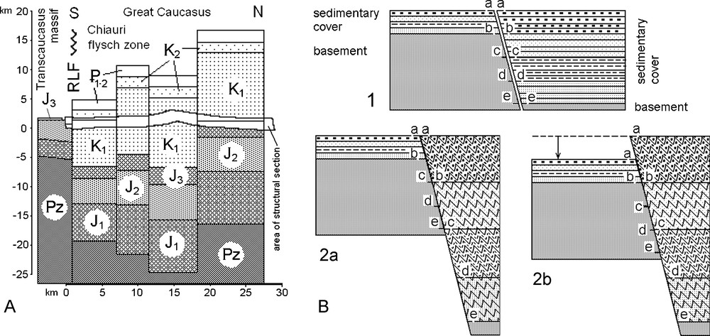
Common structure of foreland-hinterland transition zone in natural examples and in a theoretical sketch (Yakovlev, 2008e). A. Topography of main stratigraphic boundaries in the Chiauri zone (for 4 structural cells) and in adjacent Trans-Caucasus massif. Large normal offset of the top of the basement along the Racha-Lechkhum Fault is clearly seen. B. Theoretical sketch of foreland-hinterland transition zone. 1: two adjacent blocks (stable foreland to the left) after sedimentation and before folding. Initial large normal faults in the basement account for a larger sedimentary thickness in the folded block. Marked levels a-e have been placed for tracing of displacements on the next stage; 2: next stage of the structure development after near 50% of shortening in the right block. 2a: during uplift of the stable block (marked level a-a is stable); 2b: during subsidence of the stable block (marked level b-b is stable); local thrust (level a-a) in upper part of structure occurs. In both cases, the amplitude of normal faults in the basement (b-e and e-e) has increased. Masquer
Common structure of foreland-hinterland transition zone in natural examples and in a theoretical sketch (Yakovlev, 2008e). A. Topography of main stratigraphic boundaries in the Chiauri zone (for 4 structural cells) and in adjacent Trans-Caucasus massif. Large normal offset of the ... Lire la suite
Structure commune de la zone de transition entre avant-pays et arrière-pays pour un exemple naturel et sous forme de schéma principal (Yakovlev, 2008e). A. Topographie des principales limites stratigraphiques dans la zone de Chiauri (pour 4 cellules structurales) et dans le massif adjacent trans-caucasien. On observe la grande amplitude d’une faille normale type, au sommet du soubassement dans la Faille Racha-Lechkhum. B. Principal schéma de la zone de transition avant-pays–arrière-pays. 1–2 : blocs adjacents (avant-pays, stable, à gauche) à la fin de la sédimentation, avant le plissement. Le déplacement initial de la grande faille normale au niveau du sommet du soubassement a induit une plus grande épaisseur de la couverture sédimentaire dans le bloc plis ; les niveaux a-e marquent la trace du déplacement, d’un stade au suivant ; 2 : stade suivant du développement de la structure, après raccourcissement du bloc de droite aux environs de 50 %. 2a : sous la position haute du bloc stable (le niveau a-a est stable) ; 2b : sous la subsidence du bloc stable (le niveau b-b est stable) ; charriage local (niveau a-a) dans la partie haute de la structure. Dans les deux cas, l’amplitude de la faille normale au niveau du sommet du soubassement (b-e et c-e) a augmenté. Masquer
Structure commune de la zone de transition entre avant-pays et arrière-pays pour un exemple naturel et sous forme de schéma principal (Yakovlev, 2008e). A. Topographie des principales limites stratigraphiques dans la zone de Chiauri (pour 4 cellules structurales) et dans le ... Lire la suite
These results have to be commented. Thrusting of the hinterland over the foredeeps of the Greater Caucasus is an undeniable fact. However, in the proposed structural sketch, the overall thickness of one tectonic block has increased. It means that the displacement amplitudes have been different for various horizons. This is the reason why normal offset of the basement top does not exclude at all overthrusting in the upper part of the structure. Therefore this overthrusting should be regarded as a local structure, which is not representative of the main tectonic style of this orogen. It is clear that local overthrusting can occur in a much easier way within the down-faulted blocks of the foreland (Yakovlev, 2008e). The main diagnostic thin-skinned tectonic features of accretionary prisms (Dotduev, 1997) do not apply to the real basement-involved structure of the Greater Caucasus (Yakovlev, 2011). However, this specific case does not deny the possibility of the implementation of thin-skinned models to other regions.
7 Discussion - what mechanisms do we want to study?
In structural geology, the existing morphological classifications of folds and folded structures use the principle that one class of fold must relate to one mechanism of folding. As a result, the origin of a given structural feature, i.e. a fold, can be directly derived from its classification division. For example, folds of 1B type according to the J.G. Ramsay classification (Ramsay and Huber (1987), p. 349) occur under buckling mechanism. However, to explain the wide range of 1C type folds we need to combine buckling and pure shear deformation (Srivastava and Shah, 2008). The respective order of these two components is unknown. Moreover, the two processes could develop in several steps. The mechanical explanation of any sequence is difficult, and there is no independent method to choose the correct model of fold formation within the frames of such a speculative, a priori and non tectonophysical approach. Only tectonophysic modelling and strain-stress analysis could make it possible to compare quantitatively natural structures with key features deduced from rock mechanics. For instance, it sounds possible to distinguish large folds formed by lateral buckling from transversal bending ones, using the paleostress fields (Gzovsky, 1963).
We do not use the morphological classifications and a priori related mechanisms within the proposed approach. Instead, we propose to address a correct description of the deformations in a hierarchic frame of kinematic models with a sufficient data set to constrain specific kinematic mechanisms. We face two methodological possibilities. The first possibility occurs when a correct kinematic model is used as an integrative system, in which we have to settle the studied structure (folds of single viscous layer, Fig. 2). In this case, we get parameters characterizing the deformation mechanisms and strain value. The second possibility occurs when we study several pilot mechanisms in a natural case study using the same key parameters describing deformation. This makes it possible to choose the most realistic mechanism for the studied structure (for example, finding the mechanism of gravitational sliding for the Vorontsov nappe, as in Section 3 of this article).
The possibility of getting a modern balanced geometry of large structures of linear folding (3D model of the North-West Caucasus) within the whole sedimentary cover is an essential step forward. First, such reliable structure makes it possible to sort out the different types of geodynamic model. Second, they serve as an initial material for elaboration of new geodynamic scenarii.
8 Conclusions
Linear folding in thin-layered deposits of slates and flysch of the hinterland of the Greater Caucasus is a complex hierarchic structure. Mechanisms, which form different rank structures, cannot be restricted to the simplistic contradiction between lateral buckling or transversal bending processes.
Within the frame of the proposed methods, the boundaries of different rank modules to which we apply the kinematic models, are chosen in such way that specific fold forming mechanisms can be applied to these modules. It means that the geometric restrictions of folded objects and of kinematic mechanisms of its formation should be the same. The selection of module boundaries makes the basis of hierarchic systems of objects of linear folding.
The complex kinematic models used to describe the formation process linking the geometry of individual structures and the amplitude of acting model components (elementary mechanisms) are the basis of the methods that we propose for the study of different scales of structural features. This makes it possible to give a quantitative description of strain for natural objects, including the value of shortening for various structures at different scales. This set of methods that we call multi-scale strain analysis of linear folding comprises its main hierarchic levels.
The tectonophysical approach used here makes it possible to find differences in the deformation pattern of theoretical structures with different origins. The geometry of natural objects and kinematic evolutionary models allow one also to detect exactly which formation mechanism operated in each case. The present-day and reconstructed geometries of the whole sedimentary cover enable us also to test various geodynamic models.
Acknowledgments
Many aspects of this work were repeatedly discussed with Jacques Angelier from 1993 until 2008. His interest in the development of this branch of tectonophysics and his support of some results are greatly appreciated. We thank the reviewers, J. Honnorez and J.L. Mugnier, for their comments and efforts to improve the English text.