Investigation of power-law correlations within daily total ozone time series and search for a stable node through phase portrait

Parthasarathi Chakraborthy; Goutami Chattopadhyay; Surajit Chattopadhyay

doi:10.1016/j.crte.2012.12.002

External geophysics, climate

Investigation of power-law correlations within daily total ozone time series and search for a stable node through phase portrait
[Investigation sur les corrélations de loi de puissance dans des séries temporelles d’ozone total journalier et recherche d’un nœud stable dans une configuration de phase]

Présenté par : Michel Petit

Parthasarathi Chakraborthy ¹ ; Goutami Chattopadhyay ² ; Surajit Chattopadhyay ¹

¹ Pailan College of Management and Technology, 700104 Kolkata, India
² Department of Mathematics, Bengal Engineering and Science University, Shibpur, 711103 Howrah, India

Comptes Rendus. Géoscience, Volume 345 (2013) no. 2, pp. 55-61.

Résumés

Anglais
Français

In the study reported in this paper we have dealt with the intrinsic complexity of the daily total ozone time series over Mumbai, India (19°23′N, 72 15°00′E) by means of detrended fluctuation analysis and phase portrait analysis. From the detrended fluctuation analysis of first order it is revealed that the said time series is characterized by persistent power-law correlation which is stronger in shorter time scale than in the longer time scale. The phase portrait analysis is based on a non-linear autonomous system generated from regression equations; infinitely many stable nodes are found along the straight line x = 273.556 and from the behaviors of the contours, it has been revealed that the daily total ozone concentration is unlikely to go beyond 315 DU (approximately) and it is almost stable.

L’étude présentée dans cet article a concerné la complexité intrinsèque des séries temporelles quotidiennes d’ozone total au-dessus de Mumbai, Inde (19°23′N, 72 15°00′E), au moyen d’une analyse de fluctuations redressées et de portrait en phase. À partir de l’analyse de fluctuations redressées, il apparaît que la série dite temporelle est caractérisée par une corrélation en loi de puissance persistante, qui est plus forte à l’échelle de temps courts qu’à celle de temps plus longs. L’analyse de portrait de phase est basée sur un système autonome non linéaire, généré par des équations de régression; de très nombreux nœuds stables sont répertoriés le long de la ligne droite et, d’après les comportements des contours, il s’avère que la concentration journalière en ozone est peu encline à baisser au-dessous de 315 DU (approximativement) et est presque stable.

Métadonnées

Reçu le : 2012-06-11
Accepté le : 2012-12-11
Publié le : 2013-01-22

DOI : 10.1016/j.crte.2012.12.002

Keywords: Daily total ozone, Detrended fluctuation analysis, Power-law correlations, Phase portrait, Autonomous system
Mot clés : Ozone total journalier, Analyse des fluctuations redressées (DTA), Corrélations en moi de puissance, Portrait de phase, Système autonome

Affiliations des auteurs :

Parthasarathi Chakraborthy ¹ ; Goutami Chattopadhyay ² ; Surajit Chattopadhyay ¹

¹ Pailan College of Management and Technology, 700104 Kolkata, India
² Department of Mathematics, Bengal Engineering and Science University, Shibpur, 711103 Howrah, India

@article{CRGEOS_2013__345_2_55_0,
     author = {Parthasarathi Chakraborthy and Goutami Chattopadhyay and Surajit Chattopadhyay},
     title = {Investigation of power-law correlations within daily total ozone time series and search for a stable node through phase portrait},
     journal = {Comptes Rendus. G\'eoscience},
     pages = {55--61},
     publisher = {Elsevier},
     volume = {345},
     number = {2},
     year = {2013},
     doi = {10.1016/j.crte.2012.12.002},
     language = {en},
}

TY  - JOUR
AU  - Parthasarathi Chakraborthy
AU  - Goutami Chattopadhyay
AU  - Surajit Chattopadhyay
TI  - Investigation of power-law correlations within daily total ozone time series and search for a stable node through phase portrait
JO  - Comptes Rendus. Géoscience
PY  - 2013
SP  - 55
EP  - 61
VL  - 345
IS  - 2
PB  - Elsevier
DO  - 10.1016/j.crte.2012.12.002
LA  - en
ID  - CRGEOS_2013__345_2_55_0
ER  -

%0 Journal Article
%A Parthasarathi Chakraborthy
%A Goutami Chattopadhyay
%A Surajit Chattopadhyay
%T Investigation of power-law correlations within daily total ozone time series and search for a stable node through phase portrait
%J Comptes Rendus. Géoscience
%D 2013
%P 55-61
%V 345
%N 2
%I Elsevier
%R 10.1016/j.crte.2012.12.002
%G en
%F CRGEOS_2013__345_2_55_0

Parthasarathi Chakraborthy; Goutami Chattopadhyay; Surajit Chattopadhyay. Investigation of power-law correlations within daily total ozone time series and search for a stable node through phase portrait. Comptes Rendus. Géoscience, Volume 345 (2013) no. 2, pp. 55-61. doi : 10.1016/j.crte.2012.12.002. https://comptes-rendus.academie-sciences.fr/geoscience/articles/10.1016/j.crte.2012.12.002/

Version originale du texte intégral

1 Introduction

Discovery of the springtime ozone hole over Antarctica in the mid-1980s (Farman et al., 1985) shed light on ozone dynamics, especially over high and polar latitudes. The intrinsic spatial and temporal irregularity of emission concentrations, the influence of weather conditions, and uncertainties associated with initial and boundary conditions have made it a difficult task to model, calibrate and validate ozone variations (Chattopadhyay and Chattopadhyay, 2009). Sources of complexity within the total ozone have been summarized in many reports (e.g., WMO, 2010). In this regard, and studies (e.g. Chattopadhyay and Chattopadhyay-Bandyopadhyay, 2007) as follows:

• total ozone comprises tropospheric and stratospheric ozone. Both atmospheric layers contribute degrees of complexity to the corresponding ozone layer;
• formation of ozone is a complex photochemical reaction;
• formation of ozone depends upon a number of meteorological variables that may have their own complexities.

Chen et al. (1998) carried out a multidimensional phase space analysis of the observed ozone concentration and developed a powerful predictive model after investigating the trajectories on a phase space reconstructed for hourly ozone time series. Several non-linear approaches, till date, have been proposed to develop predictive models for tropospheric ozone based on the dealing with the intrinsic complexities. Some remarkable works in this direction include the studies of Jorquera et al. (1998), Koçak et al. (2000), Novara et al. (2007), Sousa et al. (2007), Heo and Kim (2004) and Feng et al. (2011). The total ozone (TO) is the integral of the ozone concentration with respect to height (Bandyopadhyay and Chattopadhyay, 2007). Association between climate and TO has been investigated by Reid et al. (1994), Varotsos et al. (1994), Efstathiou et al. (2003), Kondratyev and Varotsos (2000, 2002) and De et al. (2011). The necessity of considering the intrinsic complexity of the ozone dynamics has been emphasized in references like Kondratyev and Varotsos (1995, 2001), Varotsos et al. (2001) and Brandt et al. (2003).

In recent years, there has been growing evidence indicating that many physical systems have no characteristic length scale and exhibit long-range power-law correlations (Chen et al., 2002). Traditional approaches such as the power-spectrum and correlation analysis are suitable for stationary time series. However, many time series, which pertain to complex geophysical systems are non-stationary. This means that the mean, standard deviation and higher moments, or the correlation functions are not invariant under time translation (Stratonovich, 1981). To realize the essential dynamics of a given system, it is imperative to analyze and correctly interpret the associated time series. One of the frequent challenges is that the scaling exponent is not always constant (independent of scale) and the value of the scaling exponent fluctuates for different ranges of scales (Chen et al., 2002; Ivanov et al., 1999). Non-stationarity, which is an essential aspect of a complex variability, is often related to different trends in the signal or heterogeneous segments with different local statistical properties (Ivanov et al., 1999). The detrended fluctuation analysis (DFA) addresses this problem to accurately quantify long-range power-law correlations embedded in a non-stationary time series.

A classical approach is to use qualitative differential equations to characterize the orientation flow field by considering it as the velocity field of a particle in a dynamical system (Cohen and Herlin, 1996, 1999). Modeling the orientation flow field by a dynamical system allows us to characterize the flow field through the particles trajectories and their stationary points. Dynamical system approach is very common in bio-mathematical modeling (e.g. Jiang et al., 2007 and references therein Kelleher et al., 2003) and cosmological modeling (e.g. Jamil and Debnath, 2011; Szydłowski and Krawiec, 2003 and references therein). However, limited works are available in the area of geophysical studies, where dynamical system approach has been adopted to deal with the intrinsic complexity. We carried out a survey of the literature considering geophysical problems in the view of dynamical system. Gurol and Singer (1982) studied the kinetics of ozone decomposition in aqueous solution under dynamic conditions; ozone decomposition is a second-order reaction with respect to ozone concentration. A remarkable approach towards time series modeling of ozone concentration from dynamic point of view is by Chen et al. (1998), who emphasized the complexity of ozone dynamics due to the inherent spatial and temporal variability of emission concentrations, influence of meteorological concentrations, and uncertainties associated with the initial and boundary conditions. In Chen et al. (1998), a phase space reconstruction was presented to model and predict hourly ozone concentration time series. Jayawardena and Gurung (2000) adopted non-linear dynamical systems and linear stochastic approaches to analyze synthetic and hydrometeorological time series, where the analysis by dynamical systems approach included computation of the correlation dimension, noise reduction and non-linear prediction. Ruzmaikin et al. (2004) presented a simple dynamic model of solar variability influence on climate based on three ordinary differential equations controlled by two parameters. Different techniques and concepts of chaotic theory were adopted by Ng et al. (2007) to enhance our understanding of the phenomena of outliers for daily extreme hydrological observations.

Purpose of the present paper is twofold. We can specifically state the aims and motivation behind this study as follows: this work deals with the daily total ozone (TO) concentration over Mumbai, India. Mumbai is situated about midway on the western coast of India (19°23′N,72 15°00′E) and is a peninsular city joined to the mainland at its northern end (Venkataraman et al., 2002). Mumbai has a tropical monsoon climate with diurnal land and sea breezes of daytime onshore winds from the west and northwest and nighttime offshore winds from the north, east and northeast. An extensive analysis of various meteorological parameters and aerosol characteristics over Mumbai is available in Venkataraman et al. (2002). Two noteworthy studies by Srivastava (2004) and Srivastava et al. (2006) show the significant dominance of volatile organic compounds over Mumbai. Association between formation of ozone and VOC is discussed in Carter (1994), Kondratyev and Varotsos (2001) and Varotsos (2002). Due to the radiative and dynamic coupling between the stratosphere and troposphere, any change in the climate influences the evaluation of ozone layer through multiple changes in transport, chemical composition and thermal character (Pal, 2010). In an attempt to shed light on aforementioned complexity, scaling analysis of atmospheric data certainly is felt an important approach. Consideration of the decay of correlations in time has often been used to look into the dynamics of complex systems. A randomly forced first-order linear system with memory has an autocorrelation function decaying exponentially with lag time, but a higher order system will tend to have a different decay pattern. However, direct calculation of the autocorrelation function is affected by noise superimposed on the data (Varotsos and Kirk Davidoff, 2006). Following Varotsos and Kirk Davidoff (2006) we investigate the pattern of the decay of autocorrelation within the daily TO with increasing time lag by means of detrended fluctuation analysis (DFA). Afterwards, we have generated an autonomous system from regression equations and considered the daily TO as a dynamic system. Sources of complexity in TO has already been discussed in the works of Varotsos and Kirk Davidoff (2006), Chattopadhyay and Chattopadhyay-Bandyopadhyay (2007, 2008), De et al. (2011). This approach have been adopted because we have tried to shed light into the intrinsic complexity of the time series of daily TO by means of a phase portrait analysis.

2 Investigation of power-law correlation

2.1 Overview of detrended fluctuation analysis

Temporal correlations within the climate system are of physical and practical interest. Daily and seasonal correlations enable weather and climate prediction, and correlations on longer time scales characterize the interaction of climate components. Therefore, the analysis of correlations within the different compartments of the climate system and its realistic physical modeling are fundamental in climate research (Fraedrich and Blender, 2003). Detrended fluctuation analysis (DFA) (Peng et al., 1993) has recently been extensively implemented in the various physical processes. Several studies have reported that the DFA measure provides information that could not have been otherwise obtained, or that it is intrinsically a better measure to existing techniques (Heneghan and McDarby, 2000). The DFA is a scaling analysis method used to estimate long-range power-law correlation exponents in a time series. This method has been described in detail in the papers like Hu et al. (2001), Kantelhardt et al. (2002) and Chen et al. (2002). A brief overview of DFA is presented in this section. Peng et al. (1994) originally proposed DFA as a technique for quantifying the nature of long-range correlations. In recent years this method has become a widely used technique for the detection of long-term correlations in noisy, non-stationary time series (e.g. Bunde et al., 2002, Chen et al., 2002, Kantelhardt et al., 2006). In DFA, the data are first converted to non-stationary by generating the non-stationary profile Y(i) generated by $Y (i) = \sum_{k = 1}^{i} ϕ_{k}$ , i = 1, 2, 3,….,N (Varotsos and Kirk Davidoff, 2006), for the data series $ϕ_{k}$ of size N. Thus, the reconstructed time series has the entries:

\begin{array}{l} y (1) = [ϕ_{1} - ϕ_{a v e r a g e}] \\ y (2) = [ϕ_{1} - ϕ_{a v e r a g e}] + [ϕ_{2} - ϕ_{a v e r a g e}] \\ y (3) = [ϕ_{1} - ϕ_{a v e r a g e}] + [ϕ_{2} - ϕ_{a v e r a g e}] + [ϕ_{3} - ϕ_{a v e r a g e}] \\ ⋮ \\ y (N) = \sum_{k = l}^{N} [ϕ_{k} - ϕ_{a v e r a g e}] \end{array}

(1)

The integration:

• exaggerates the non-stationarity of the original data;
• reduces the noise level;
• generates a time series corresponding to the construction of a random walk that has the values of the original time series as increments (Varotsos and Kirk Davidoff, 2006).

The new time series, however, still preserves information about the variability of the original time series. In the next step, we divide the reconstructed time series Y(i) into N_l = int(N/l) non-overlapping segments of equal length l. The length N of the series being not a multiple of the considered timescale l, a small part at the end of the reconstructed time series may remain outside the segments generated above. In order not to disregard this part of the series, Kantelhardt et al. (2006) proposed to repeat the same procedure starting from the opposite end. Hence, 2N_l segments are obtained altogether. For each of the 2N_l blocks by fitting a polynomial of order n to the data we determine the variance for each block as (Kantelhardt et al., 2006)

σ (v, l) = \frac{1}{l} \sum_{i = 1}^{l} {[Y ((v - 1) l + i) - p_{v} (i)]}^{2}

(2)

where v varies from 1 to 2N_l and p_v(i) is the fitting polynomial representing the local trend in the segment. The local trend in each block is defined to be a linear least-squares fit to the samples in that block. Linear, quadratic, cubic, or higher-order polynomials can be used in the fitting procedure. When linear polynomials are used, the fluctuation analysis is called DFA1, for quadratic polynomials we have DFA2. In the present work, we have experimented DFA1. A detrended signal is defined for each block as the difference between the original signal and the local trend for that block and the detrended fluctuation function is derived as (Kantelhardt et al., 2006)

F^{2} (l) = \frac{1}{2 N_{l}} \sum_{v = 1}^{2 N_{l}} σ (v, l)

(3)

The detrended fluctuation function is computed for different values of l. It has been shown by Buldyrev et al. (1995) that F(l) varies as a power-law in l, for sequences with power-law long-range correlations. This means that if data series ϕ_k is characterized by long-term power-law correlation, F(l) increases, for large values of l, by a power-law, notably F(l)αl^α (Kantelhardt et al., 2006). When the autocorrelation function decreases faster than 1/l in time, we asymptotically have F(l)αl^α. Conventionally, an exponent α ≠ 1/2 in a certain range of l values implies the existence of long-range correlations in that time interval. In Varotsos (2005), the types of correlation present in a time series implied by the value of α is thoroughly discussed. A straight line fit to the log-log plot of the log-log graph indicates statistical self-affinity expressed as F(l)αl^α. The scaling exponent α is calculated as the slope of a straight line fit to the log-log graph of l against F(l5) using least-squares. If 0.5 < α ≤1, then persistent long-range power-law correlations exist in the time series, if 0 < α < 0.5, then the time series is characterized by power-law anticorrelations (antipersistence) and when 1 < α < 1.5, then there are correlations again. A Brownian noise is indicated by α = 1.5(Varotsos, 2005).

2.2 Discussion on the data under consideration

In the present work, we have dealt with the daily total ozone (TO) concentration over Mumbai, India. The data are derived from the measurements made by the Earth Probe Total Ozone Mapping Spectrometer (EP/TOMS) and are available at the website http://ftp://jwocky.gsfc.nasa.gov/pub/eptoms/data/overpass/OVP206_epc.txt. For executing DFA we have considered the daily TO spanned over 1999–2000. Based on the discussion presented in the previous section we have first detrended the time series of daily TO and then divided the data series into several non-overlapping boxes of different sizes. The box size l has varied from 2 to 50. For each box size we have removed the local trend by means of removing the first order as well as second order trend. This means that, in Eq. (2) we have used pv(i) in the linear form. Thus, DFA1 is executed. For different ranges of the box length we fit straight lines to the log-log graph of l against F(l) by least square method. Results are presented in the Table 1. It is observed from Table 1 and from the Fig. 1(a-c) that the scaling exponent α is always above 0.5 and never becomes equal to 1.5. Hence, it is concluded that for the time interval ranging from about 2 days to more than one month, the time series of daily TO over Mumbai is characterized by persistent power-law correlations. However, from the decreasing behavior of the R² it may be interpreted that the power-law correlation is stronger in shorter time scale than in the longer time scale. Moreover, no prominent periodicity is observed in this power-law correlation. Based on the observation of Varotsos and Kirk Davidoff (2006) this may be interpreted as an indicator of existence of dynamical links between long and short time-scale behavior. In the subsequent section, we shall consider the said daily TO time series as a dynamic system by generating a set of differential equations and subsequently studying the behaviors of the critical points within the phase portrait.

Range of l	Straight line fit	Value of α	Nature of the series self-correlations
2 to 15	y = 1.4436x + 1.4378 (R² = 0.9587)	1.4436	Persistent long-range power-law correlations
2 to 30	y = 1.0238x + 1.7741 (R² = 0.8006)	1.0238	Persistent long-range power-law correlations
2 to 45	y = 0.8158x + 1.9676 (R² = 0.3242)	0.8158	Persistent long-range power-law correlations

Fig. 1
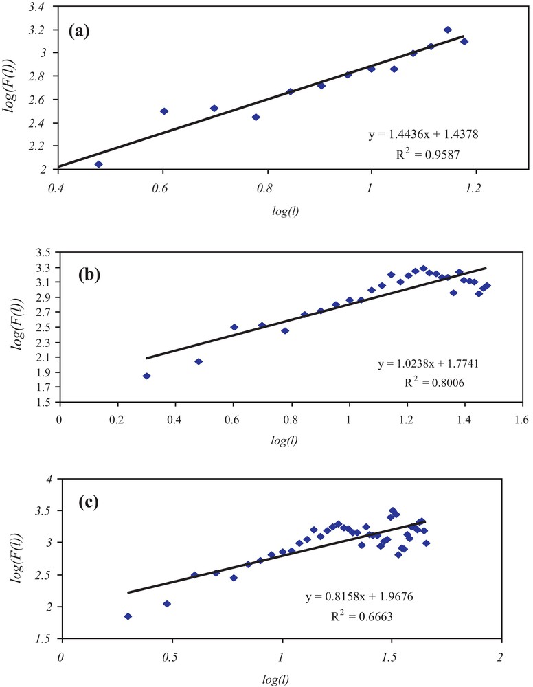
Straight line fits to various ranges of l. The first panel corresponds to the range 2 to 15, the second panel corresponds to the range 2 to 30 and the third panel corresponds to the range 2 to 45.
La ligne droite est ajustée aux différentes amplitudes de l. Le premier panneau correspond à la gamme de 2 à 15, le deuxième à la gamme de 2 à 30 et le troisième à la gamme de 2 à 45.

3 Dynamical system approach

Two systems of first order autonomous differential equations are said to be topologically equivalent if an invertible mapping exists between one phase portrait onto the other while preserving the orientation of the trajectories. Phase portraits are created using isoclines, vector fields, and eigenvectors. A non-linear autonomous system is considered in the form (Lynch, 2010):

\dot{x} = P (x, y)

(4a)

\dot{y} = Q (x, y)

(4b)

where at least one of P and Q is non linear in x and y. The critical points (u, v) is obtained by solving

\dot{x} = 0 = \dot{y}

. The non-linear system is linearized by computing the following Jacobian matrix at every critical point (u, v):

J_{(u, v)} = (\begin{array}{l} \frac{\partial P}{\partial x} \frac{\partial P}{\partial y} \\ \frac{\partial Q}{\partial x} \frac{\partial Q}{\partial y} \end{array})

(5)

In the present work, we shall view the daily TO time series as a dynamical system. To do the same, it is needed to generate two-dimensional linear differential equations in the forms presented in (1a) and (1b). Now we consider polynomial regressions as:

x = ξ (t)

(6)

y = η (x)

(7)

where ξ(t) and η(x) denote second degree polynomials in t and x respectively, t denotes time, x denotes the observations corresponding to t, and y denotes the time series lagged by 1 time point. By means of least square regression we estimate the regression constants and coefficients as:

a = 250.91, b = 0.1346, c = –0.0002, d = –283.66, e = 3.2806 and f = –0.0045.

Subsequently, the non-linear autonomous system is generated as:

\frac{d x}{d t} = {[b^{2} - 4 a c + 4 c x]}^{1 / 2}

(8)

\frac{d y}{d t} = {[b^{2} e^{2} + 4 c e^{2} (x - a) + 4 b^{2} f (y - d) + 16 c f (- a + x) (- d + y)]}^{1 / 2}

(9)

\frac{d x}{d t} = 0

occurs when x = 273.556. With this value of x, the

\frac{d y}{d t}

happens to be 0 for any value of y. Thus, we get infinitely many critical points along the straight line x = 273.556. Since we are considering density of TO, we shall consider y to be positive. The Jacobian matrix comes out to be:

J = (\begin{array}{l} \frac{2 c}{\sqrt{b^{2} - 4 a c + 4 c x}} 0 \\ \frac{2 c \sqrt{e^{2} - 4 d f + 4 f y}}{\sqrt{b^{2} - 4 a c + 4 c x}} \frac{2 f \sqrt{b^{2} - 4 a c + 4 c x}}{\sqrt{e^{2} - 4 d f + 4 f y}} \end{array})

(10)

Using the values of the regression constants and parameters the eigenvalues are:

λ_{1} = - \frac{0.0004}{\sqrt{0.218845 - 0.0008 x}}

(11)

λ_{2} = - \frac{0.009 \sqrt{0.218845 - 0.0008 x}}{\sqrt{5.65646 - 0.015 y}}

(12)

Since both of the eigenvalues are real and negative along for all of the critical points, we conclude that the eigenvectors represent stable situations that the system converges towards, and the intersection is a stable node. For a system of n first-order ordinary differential equations (or more generally, Pfaffian forms), the 2n-dimensional space consisting of the possible values of ( $x_{1}, {\dot{x}}_{1}, x_{2}, {\dot{x}}_{2} ......, x_{n}, {\dot{x}}_{n}$ ) is known as its phase space (Weisstein, 2011). For a function with 2 degrees of freedom, the 2-dimensional phase space that is accessible to the function or object is called its phase plane. A phase portrait is a plot of multiple phase curves corresponding to different initial conditions in the same phase plane (Weisstein, 2011). For the present dynamical system, the phase portrait is presented in Fig. 2. We find that all the trajectories are directed towards the line x = 273.556 and the situation being stable it may be interpreted that the daily TO over Mumbai has the tendency to be in the vicinity of 273 DU. Now we consider the contours within the phase portrait. These contours pertain to different initial conditions. From the nature of the contours we see that all of them are converging towards the point (273, 310). The values of y are first increasing with increase in x. This means that the concentration of daily TO is increasing as well as the concentration at time point lagged by 1 is also increasing. In the vicinity of (273, 315), both variables get confined and thus it may be interpreted that the concentration of the daily TO concentration is unlikely to go beyond 315 DU (approximately) and it is almost stable.

Fig. 2
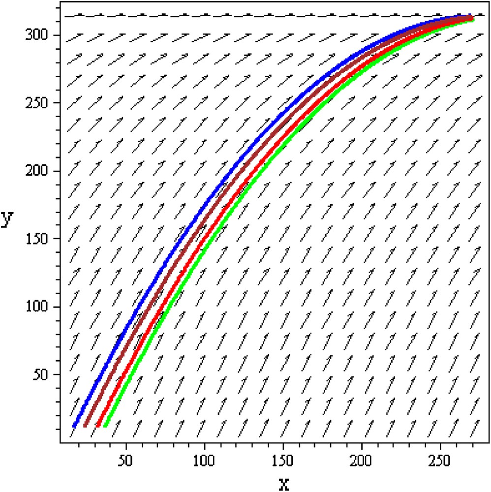
The phase portrait. Here, the horizontal axis corresponds to x_t and the vertical axis corresponds to x_t+1 For convenience, these are denoted as x and y respectively.
Portrait de phase.L’axe horizontal correspond à x_t et l’axe vertical à x_t+l. Par commodité, ces axes sont appelés x et y respectivement.

4 Concluding remarks

In the study explained in the previous sections, we have dealt with the intrinsic complexity of the daily total ozone time series over Mumbai, India by means of detrended fluctuation analysis and phase portrait analysis. In the introductory part of the paper we have thoroughly discussed the motivation behind adopting the above methodologies to deal with the daily total ozone over Mumbai, where the atmospheric environment is dominated by volatile organic compounds. The detrended fluctuation analysis has been implemented by using first order polynomials to the non-overlapping blocks. It is revealed that for the time interval ranging from about 2 days to more than one month, the time series of daily total ozone over Mumbai is characterized by persistent long-range power-law correlations. However, from the decreasing behavior of the coefficient of determination with block length it has been understood that the power-law correlation is stronger in shorter time scale than in the longer time scale. In the next part of the study, we have created an autonomous system by means of ordinary differential equations based on non-linear regression equations fit to the time series first with time t as the independent variable and the corresponding observation x_t as the dependent variable and then by x_t as the independent and x_t+1 as the dependent variable. Subsequently we have created the phase portrait where it has been found that there are infinitely many stable nodes along the vertical axis. Observing the fact that all the trajectories on the phase portrait are directed towards the line x = 273.556 and the situation being stable it may be interpreted that the daily TO over Mumbai has the tendency to be in the vicinity of 273 DU. It is further observed that all of contours along the phase portrait are converging towards the point (273, 310). This leads us to conclude that the concentration of daily total ozone is increasing as well as the concentration at time point lagged by 1 is also increasing. In the vicinity of (273, 315), both variables get confined and thus it may be interpreted that the concentration of the daily total ozone concentration is unlikely to go beyond 315 DU (approximately) and it is almost stable. Based on the time series under consideration we have constructed a phase portrait and obtained a stable node based on the autonomous system. The trajectories are tending towards the said point and hence it is an approximate stable node. If longer time series are considered then more complexity would be explored and we propose to study this in future.

Acknowledgement

The authors are thankful to the reviewers for their thoughtful suggestions to enhance the quality of the paper.

Bibliographie

[Bandyopadhyay and Chattopadhyay, 2007] G. Bandyopadhyay; C. Chattopadhyay Single hidden layer artificial neural network models versus multiple linear regression model in forecasting the time series of total ozone, Int. J. Environ. Sci. Tech., Volume 4 (2007), pp. 141-149

[Brandt et al., 2003] J. Brandt; J. Christensen; L.M. Frohn; R. Berkowicz Air pollution forecasting from regional to urban street scale – implementation and validation for two cities in Denmark, Phys. Chem. Earth, Volume 28 (2003) no. 8, pp. 335-344

[Buldyrev et al., 1995] S.V. Buldyrev; A.L. Goldberger; S. Havlin; R.N. Mantegna; M.E. Matsa; C.K. Peng; M. Simons; H.E. Stanley Long-range correlation properties of coding and noncoding DNA sequences: GenBank analysis, Phys. Rev. E., Volume 51 (1995), pp. 5084-5091

[Bunde et al., 2002] A. Bunde; J. Kropp; H.J. Schellnhuber The science of disaster: climate disruptions, market crashes, and heart attacks, Springer, New York, 2002

[Carter, 1994] W.P.L. Carter Development of ozone reactivity scales for volatile organic compounds, J. Air Waste Manage. Assoc., Volume 44 (1994) no. 7, pp. 881-899

[Chattopadhyay and Chattopadhyay-Bandyopadhyay, 2007] S. Chattopadhyay; G. Chattopadhyay-Bandyopadhyay Artiﬁcial Neural Network versus autoregressive approach: prediction of total ozone time series, Model Assist. Stat. Appl., Volume 2 (2007), pp. 107-120

[Chattopadhyay and Chattopadhyay-Bandyopadhyay, 2008] G. Chattopadhyay-Bandyopadhyay; S. Chattopadhyay A probe into the chaotic nature of total ozone time series by correlation dimension method, Soft Computing, Volume 12 (2008), pp. 1007-1012

[Chattopadhyay and Chattopadhyay, 2009] G. Chattopadhyay; C. Chattopadhyay Autoregressive forecast of monthly total ozone concentration: a neurocomputing approach, Comput. Geosci., Volume 35 (2009), pp. 1925-1932

[Chen et al., 1998] J.L. Chen; S. Islam; P. Biswas Nonlinear dynamics of hourly ozone concentrations: nonparametric short term prediction, Atmos. Environ., Volume 32 (1998), pp. 1839-1848

[Chen et al., 2002] Z. Chen; P.C. Ivanov; K. Hu; H.E. Stanley Effect of nonstationarities on detrended fluctuation analysis, Phys. Rev. E, Volume 65 (2002), p. 041107 | DOI

[Cohen and Herlin, 1996] I. Cohen; I. Herlin Optical flow and phase portrait methods for environmental satellite image sequences, Lecture Notes in Comp. Sci. (Springer), Volume 1065/1996 (1996), pp. 141-150 | DOI

[Cohen and Herlin, 1999] I. Cohen; I. Herlin Non uniform multiresolution method for optical flow and phase portrait models: environmental applications, Intern. J. Computer Vision, Volume 33 (1999), pp. 29-49

[De et al., 2011] S.S. De; G. Chattopadhyay; B. Bandyopadhyay; S. Paul A neurocomputing approach to the forecasting of monthly maximum temperature over Kolkata, India using total ozone concentration as predictor, C. R. Geoscience, Volume 343 (2011), pp. 664-676

[Efstathiou et al., 2003] M.N. Efstathiou; C.A. Varotsos; R.P. Singh; A.P. Cracknell; C. Tzanis On the longitude dependence of total ozone trends over middle latitudes, Intern. J. Remote Sensing, Volume 24 (2003), pp. 1361-1367

[Farman et al., 1985] J.C. Farman; B.G. Gardiner; J.D. Shanklin Large losses of total ozone over Antarctic reveal seasonal ClOx/NOx interactions, Nature, Volume 315 (1985), pp. 207-210

[Feng et al., 2011] Y. Feng; W. Zhang; D. Sun; L. Zhang Ozone concentration forecast method based on genetic algorithm optimized back propagation neural networks and support vector machine data classification, Atmos. Environ., Volume 45 (2011), pp. 1979-1985

[Fraedrich and Blender, 2003] K. Fraedrich; R. Blender Scaling of Atmosphere and Ocean Temperature Correlations in Observations and Climate Models, Phys. Rev. Lett., Volume 90 (2003) | DOI

[Gurol and Singer, 1982] M.D. Gurol; P.C. Singer Kinetics of ozone decomposition – A dynamic approach, Environ. Sci. Tech., Volume 16 (1982), pp. 377-383

[Heneghan and McDarby, 2000] C. Heneghan; G. McDarby Establishing the relation between detrended fluctuation analysis and power spectral density analysis for stochastic processes, Phys. Rev. E, Volume 62 (2000), pp. 6103-6110

[Heo and Kim, 2004] J.-S. Heo; D.-S. Kim A new method of ozone forecasting using fuzzy expert and neural network systems, Sci. Total Environ., Volume 325 (2004), pp. 221-237

[Hu et al., 2001] K. Hu; P.C. Ivanov; Z. Chen; P. Carpena; H.E. Stanley Effect of Trends on Detrended Fluctuation Analysis, Phys. Rev. E, Volume 64 (2001), p. 011114 | DOI

[Ivanov et al., 1999] P.C. Ivanov; A. Bunde; L.A.N. Amaral; S. Havlin; J. Fritsch-Yelle; R.M. Baevsky; H.E. Stanley; A.L. Goldberger Sleep-wake differences in scaling behavior of the human heartbeat: analysis of terrestrial and long-term space flight data, Europhys. Lett., Volume 48 (1999), pp. 594-600

[Jamil and Debnath, 2011] M. Jamil; U. Debnath Interacting modified Chaplygin gas in loop quantum cosmology, Astrophys. Space Sci., Volume 333 (2011), pp. 3-8

[Jayawardena and Gurung, 2000] A.W. Jayawardena; A.B. Gurung Noise reduction and prediction of hydrometeorological time series: dynamical systems approach vs. stochastic approach, J. Hydrol., Volume 228 (2000), pp. 242-264

[Jiang et al., 2007] G. Jiang; Q. Lu; L. Qian Complex dynamics of a Holling type II prey–predator system with state feedback control, Chaos, Solitons Fractals, Volume 31 (2007), pp. 448-461

[Jorquera et al., 1998] H. Jorquera; R. Perez; A. Cipriano; A. Espejo; M.V. Letelier; G. Acuna Forecasting ozone daily maximum levels at Santiago, Chile, Atmos. Environ., Volume 32 (1998), pp. 3415-3424

[Kantelhardt et al., 2002] J.W. Kantelhardt; S.A. Zschiegner; E. Koscielny-Bunde; A. Bunde; S. Havlin; H.E. Stanley Multifractal detrended fluctuation analysis of nonstationary time series, Physica A, Volume 316 (2002), p. 87 | DOI

[Kantelhardt et al., 2006] J.W. Kantelhardt; E. Koscielny-Bunde; D. Rybski; P. Braun; A. Bunde; S. Havlin Long-term persistence and multifractality of precipitation and river runoff records, J. Geophys. Res., Volume 111 (2006), p. D01106 | DOI

[Kelleher et al., 2003] B.P. Kelleher; S.F. Oppenheimer; F.X. Han; K.O. Willeford; M.J. Simpson; A.J. Simpson; W.L. Kingery Dynamical systems and phase plane analysis of protease – clay interactions, Langmuir, Volume 19 (2003) no. 22, pp. 9411-9417 | DOI

[Koçak et al., 2000] K. Koçak; L. Şaylan; O. Şen Nonlinear time series prediction of O₃ concentration in Istanbul, Atmos. Environ., Volume 34 (2000), pp. 1267-1271

[Kondratyev and Varotsos, 1995] K.Y. Kondratyev; C.A. Varotsos Atmospheric ozone variability in the context of global change, Intern. J. Remote Sensing, Volume 16 (1995), pp. 1851-1881

[Kondratyev and Varotsos, 2000] K.Y. Kondratyev; C. Varotsos Atmospheric ozone variability: implications for climate change, human health and ecosystems, Springer, New York, 2000

[Kondratyev and Varotsos, 2001] K.Y. Kondratyev; C.A. Varotsos Global tropospheric ozone dynamics Part I: tropospheric ozone precursors. Part II: numerical modeling of tropospheric ozone variability, Environ. Sci. Pollut. Res., Volume 8 (2001), pp. 57-62

[Kondratyev and Varotsos, 2002] K.Y. Kondratyev; C. Varotsos Remote sensing and global tropospheric ozone observed dynamics, Intern. J. Remote Sensing, Volume 23 (2002), pp. 159-178

[Lynch, 2010] Lynch S. 2010. Dynamical systems with applications using Maple™. Birkhäuser Boston, a part of Springer Science + Business Media.

[Ng et al., 2007] W.W. Ng; U.S. Panu; W.C. Lennox Chaos based Analytical techniques for daily extreme hydrological observations, J. Hydrol., Volume 342 (2007), pp. 17-41

[Novara et al., 2007] C. Novara; V. Marialuisa; G. Finzi Non linear models to forecast ozone peaks, Air Pollut. Model. Applic., Volume XVII (2007) no. 11, pp. 721-723 | DOI

[Pal, 2010] C.M. Pal Variability of total ozone over India and its adjoining regions during 1997–2008, Atmos. Environ., Volume 44 (2010), pp. 1927-1936

[Peng et al., 1993] C.K. Peng; S.V. Buldyrev; S. Havlin; M. Simons; H.E. Stanley; A.L. Goldberger Finite size effects on long-range correlations: implications for analyzing DNA sequences, Phys. Rev. E, Volume 47 (1993), pp. 3730-3733

[Reid et al., 1994] S.J. Reid; G. Vaughan; N.J. Mitchell; I.T. Prichard; H.J. Smit; T.S. Jorgensen; C. Varotsos; H. De Backer Distribution of the ozone laminae during EASOE and the possible influence of inertia-gravity waves, Geophys. Res. Lett., Volume 21 (1994), pp. 1479-1482

[Ruzmaikin et al., 2004] A. Ruzmaikin; J.K. Lawrence; A.C. Cadavid A simple model of solar variability influence on climate, Adv. Space Res., Volume 34 (2004), pp. 349-354

[Sousa et al., 2007] S.I.V. Sousa; F.G. Martins; M.C.M. Alvim-Ferraz; M.C. Pereira Multiple linear regression and artificial neural networks based on principal components to predict ozone concentrations, Environ. Model. Softw., Volume 22 (2007), pp. 97-103

[Srivastava, 2004] A. Srivastava Source apportionment of ambient VOCS in Mumbai city, Atmos. Environ., Volume 38 (2004), pp. 6829-6843

[Srivastava et al., 2006] A. Srivastava; A.E. Joseph; S. Devotta Volatile organic compounds in ambient air of Mumbai – India, Atmos. Environ.t, Volume 40 (2006), pp. 892-903

[Stratonovich, 1981] R.L. Stratonovich, Topics in the Theory of Random Noise, 1, Gordon & Breach, New York, 1981

[Szydłowski and Krawiec, 2003] M. Szydłowski; A. Krawiec Dynamical system approach to cosmological models with a varying speed of light, Phys. Rev. D, Volume 68 (2003), p. 063511 | DOI

[Varotsos, 2002] C. Varotsos The southern hemisphere ozone hole split in 2002, Environ. Sci. Pollut. Res., Volume 9 (2002), pp. 375-376

[Varotsos, 2005] C. Varotsos Power-law correlations in column ozone over Antarctica, Intern. J. Remote Sensing, Volume 26 (2005), pp. 3333-3342

[Varotsos and Kirk Davidoff, 2006] C. Varotsos; D. Kirk Davidoff Long-memory processes in ozone and temperature variations at the region 60^o S–60 ^o N, Atmos. Chem. Phys., Volume 6 (2006), pp. 4093-4100

[Varotsos et al., 1994] C. Varotsos; P. Kalabokas; G. Chronopoulos Association of the laminated vertical ozone structure with the lower-stratospheric circulation, J. Appl. Meteorol., Volume 33 (1994), pp. 473-476

[Varotsos et al., 2001] C. Varotsos; K.Y. Kondratyev; M. Efstathiou On the seasonal variation of the surface ozone in Athens, Greece, Atmos. Environ., Volume 35 (2001), pp. 315-320

[Venkataraman et al., 2002] C. Venkataraman; K. Reddy; S. Josson; M.S. Reddy Aerosol size and chemical characteristics at Mumbai, India, during the INDOEX-IFP (1999), Atmos. Environ., Volume 36 (2002), pp. 1979-1991

[Weisstein, 2011] Weisstein E. W. 2011. Phase Portrait. From MathWorld – A Wolfram Web Resource. http://mathworld.wolfram.com/PhasePortrait.html [accessed on 25th October, 2011].

[WMO, 2010] WMO (World Meteorological Organization), 2010. Scientific Assessment of Ozone Depletion: 2010. Global Ozone Research and Monitoring Project-Report N^o 52, Geneva.

Commentaires - Politique

Ces articles pourraient vous intéresser

Spatial and temporal variability in maximum, minimum and mean air temperatures at Madhya Pradesh in central India

Darshana Duhan; Ashish Pandey; Krishan Pratap Singh Gahalaut; ...

C. R. Géos (2013)

A neurocomputing approach to the forecasting of monthly maximum temperature over Kolkata, India using total ozone concentration as predictor

Syam Sundar De; Goutami Chattopadhyay; Bijoy Bandyopadhyay; ...

C. R. Géos (2011)

The improvement of the Morlet wavelet for multi-period analysis of climate data

Hua Yi; Hong Shu

C. R. Géos (2012)