

1 Introduction
Understanding the roles of predisposed conditions in controlling the type and pattern of landslides is important for determining the spatial probability of landslide occurrence (i.e., landslide susceptibility) (Carrara et al., 1999; Guzzetti et al., 1999; Soeters and van Westen, 1996). Moreover, significant insights regarding the roles of predisposing landslide factors when evaluating landslide susceptibility (LS) are important for decision makers, planners, and engineers. To mitigate susceptibility, it is important to know how specific predisposing factors act on slope instability.
During the last few decades, many researchers have developed landslide susceptibility maps that use different statistical analysis methods (van Westen et al., 2008 and references therein). Independent of the applied analysis complexity, all statistical methods were based on the common assumption that “the past and the present are the key to the future” (Carrara et al., 1995). Thus, the probability of a landslide occurring within a landslide free area was determined by comparing the geo-environmental characteristics of these areas with those in areas where landslides have occurred (Fell et al., 2008; Kanungo et al., 2009). For all statistical methods, the conceptual knowledge behind the LS zonation included the following (Carrara et al., 1995; Van Den Eeckhaut et al., 2006):
- • the knowledge of landslide distributions;
- • the definition of a set of factors that can be used to predict the occurrence of a landslide;
- • the assessment of statistical relationships between the predisposing factors and the occurrence of landslides.
The definition of landslide-predisposing factors is not obvious and requires detailed knowledge of the geomorphological evolution of the study areas. Furthermore, susceptibility analysis at the basin scale implies that the geo-environmental factors have a low cost/benefits ratio (i.e., the geo-environmental factors that perform more efficiently in large areas) (Soeters and van Westen, 1996; van Westen et al., 2008). Among the geo-environmental factors with a low cost/benefits ratio, the lithology, slope angle, distance to streams, and distance to tectonic lineaments are widely accepted as important factors that are related to the occurrence of landslides (Cevik and Topal, 2003; Sterlacchini et al., 2011; Yalcin et al., 2011). Conversely, the importance of slope face orientation (slope aspect) in the occurrence of landslides is debated. Some authors consider slope aspect as one of the most important predisposing factors for landslides (Galli et al., 2008; Lee, 2005; Yalcin and Bulut, 2007). However, others limit the importance of slope aspect to certain types of landslides (Atkinsons and Massari, 1998; Luzi and Pergalani, 1999), whereas several authors have indicated that slope aspect is unable to predict the development of landslides (Ayalew and Yamagishi, 2004; Cevik and Topal, 2003; Ohlmacher and Davis, 2003). The varying effect of slope aspect on landslide distribution is evident when comparing more recent landslide susceptibility studies that use robust multivariate methods (Atkinsons and Massari, 2011; Blahut et al., 2010; Das et al., 2010; De Rose, 2013; He et al., 2012; Yalcin et al., 2011).
Overall, the role that the slope aspect plays in predicting landslides remains unclear.
This study does not attempt to solve this problem completely. However, it serves to highlight several considerations that could be useful for understanding the role that slope aspect plays in the spatial distribution of landslides. In this study, bivariate and multifactor analysis between slope aspect and landslide distribution was conducted in two basins that are situated at similar latitudes and characterized by different lithological conditions. Moreover, to compare the results from the two basins, the geo-environmental factors were statistically analyzed in the basins that had the most important predisposing landslide factors (i.e., lithology, slope angle, and distance to streams and to tectonic lineaments).
2 Study areas
The statistical analyses were applied to the Milia and Roglio basins that occur in the southern and central regions of Tuscany (Italy), respectively (Fig. 1).
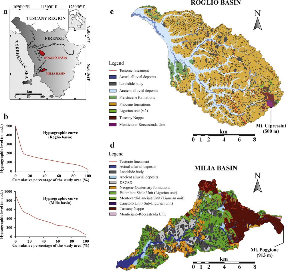
Location of the study areas (a), their hypsographic (b), and geological (c, d) characteristics.
The Milia basin covers an area of 101 km2 with an average elevation of 336 m above sea level (ranging from 39 to 913 m with a standard deviation of 167.5 m). The altitude increases from the western to eastern sectors of the basin with a morphological-structural high at Poggione Mountain (913 m). Most of the higher order streams (Strahler, 1952) follow a NE–SW direction and exhibit intense vertical erosion in the northeastern sector of the basin. In contrast, lateral erosion dominates in the western sector.
The Roglio basin covers 160 km2 with an average elevation of 130.9 m above sea level (ranging from 20 to 500 m with a standard deviation of 72.1 m). The basin has a predominantly hilly morphology without very steep slopes. A hypsographic curve is typical of landscapes in which the connection areas between the valley floor and the valley slopes are extended. This value increases to a maximum of 500 m near the morphological-structural high of Cipressini Mountain. The erosive processes that are associated with lateral river actions occur with notable intensities along the Roglio torrent between the central areas of the basin and up to its confluence with the Era River (one of the main tributaries of the Arno River, Fig. 1).
In the study basins, compressional events that occurred before and during the collisional Apennine episode resulted in a complex sheet stack where the Ligurian units (s.l.) were placed above the Tuscany Nappe (Costantini et al., 2000, 2002; Fig. 1). These allochthonous units are characterized by siltitic, argillitic, and fine arenitic formations and by shale formations with inter-bedded basalts, gabbros, and serpentinites. The Tuscany Nappe is mainly represented by a Mesozoic carbonate succession with few Cretaceous–Tertiary turbiditic outcrops and a hemipelagic sequence. The Tuscany Nappe is overthrust above the Monticiano-Roccastrada unit (“Autochthon” Metamorphic unit), which is characterized by alternating phyllites and marbles. After the emplacement of the Ligurian and Tuscan units, the Neogene–Quaternary formations were deposited in each basin. The Neogene–Quaternary formations are representative of continental and coastal-marine environments and are characterized by sandy clays and sandy conglomerates.
Ligurian units mostly characterize the Milia basin, whereas in the Roglio basin Neogene–Quaternary formations are the more extensive outcrops (Fig. 1).
In both basins, the allochthonous units underwent a complex deformation history, where at least three folding phases were related to the pre- and sin-collisional events. Post-collisional deformations have been extensional since the Middle Miocene and have resulted in the partial collapse of the Apennines (Carmignani et al., 1994). Differential uplift, lowering, and tilting phenomena have occurred since the Middle Pleistocene and have caused the rapid sinking of the hydrographic network.
The morphology of the study areas is strongly conditioned by numerous mass movements, including translational slides, rotational slides, and flows (Cruden and Varnes, 1996). In the Milia basin, many deep-seated gravitational slope deformations (DSGSD) (Dramis and Sorriso-Valvo, 1994) are present. These deformations are potentially related to the Pleistocene tectonic setting and base level lowering. From a classification point of view, these DSGSDs could be considered similar to Sackung (Capitani et al., 2013). Most of these DSGSDs are involved in landslide processes.
In the Roglio basin, the dominance of clayey and clayey-sandy lithologies resulted in genesis, a smooth landscape, and the development of badlands. The spatial distribution of the diffuse badlands is related to the slope aspect (Fig. 2). In fact, among the predisposing factors that were suggested in the literature, the southern-facing slope is most favorable in semiarid regions. In this case, more rapid drying during sunny conditions lead to larger expansion/contraction cycles in the slope regolith, which results in superficial cracks (Alexander et al., 2008; Cantón et al., 2001; Gallart et al., 2012a,b; Torri, 1996). During rainfall events, rainwater percolates downward quickly in the superficial cracks as the slope load increases and the sheer strength of the slope material decreases.
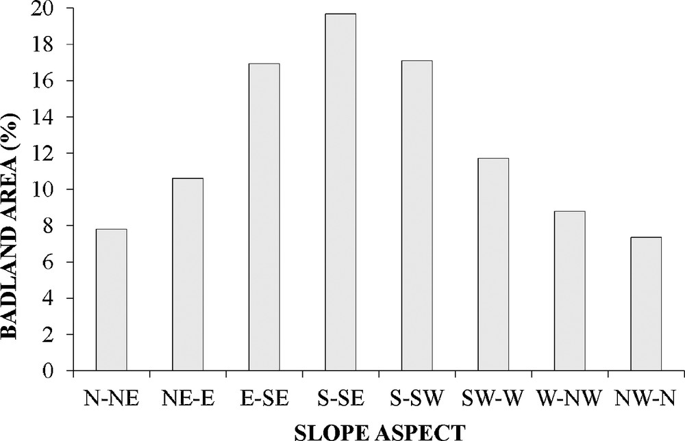
The distribution of the badlands with respect to the slope aspect values.
In both basins, many landslides have developed from older landslides. Because several aspects can affect rainfall, discontinuities and sunlight exposure (Dai et al., 2001, 2002), the stabilities of the slope debris are progressively weakened. The presence of landslide bodies can be important for influencing the distribution of new landslides that are related to slope aspect.
3 Methods
3.1 Bivariate conditional analysis
The conditional analysis is based on Bayes’ Theorem (Carrara et al., 1995), which states that the probability of that event A (dependent event) occurs depends on the occurrence of event B (predisposing event). This probability is determined as the ratio between the probabilities of the two events occurring simultaneously and the occurrence of the conditioning event P(B). For independent events, the probability of is equivalent to the probability P(A) of event A. Thus, the dependency between events A and B increases as the difference between the probabilities of and P(A) increases. When analyzing the degree of dependence between two spatial variables, the probability that the dependent variable occurs is quantified as the ratio of the area (frequency) that this variable assumes in presence of the predisposing variable (joined frequency) to the overall area (frequency) of the predisposing variable.
In the presence of qualitative-nominal and quantitative spatial variables, the variables must be subdivided spatially into classes (modalities or unique condition units) (Giudici, 2005). In this case, the degree of spatial dependence between the two variables is determined by analyzing a contingency table (Fabbris, 1997; Giudici, 2005), in which the joined frequencies (nij) of the two variable modalities (Yi, Xi) are reported (Table 1). From the contingency table, two variables are independent if the following conditions are met:
| (1) |
| (2) |
Theoretical contingency table for two variables dependence analysis.
| Variable | X 1 | X 2 | X 3 | X 4 | X 5 | Total |
| Y1 | n 11 | n 12 | n 13 | n 14 | n 15 | Ny 1 |
| Y2 | n 21 | n 22 | n 23 | n 24 | n 25 | Ny 2 |
| Total | Nx 1 | Nx 2 | Nx 3 | Nx 4 | Nx 5 | N Tot. |
Generally, natural variables are not completely dependent or independent. To quantify the degree of dependence of natural variables, statistical coefficients are generally obtained from contingency tables. Among these coefficients, the Pearson's coefficient (χ2) and the Cramér's coefficient (V) have been used in recent LS studies (Dewitte et al., 2010; Jiménez-Perálvarez et al., 2009; Van Den Eeckhaut et al., 2006).
Based on the theoretical contingency table (Table 1), Pearson's χ2 can be used to evaluate the degree of dependence between two variables (Y, X). This evaluation is conducted by determining the difference between the observed joined frequencies (nij) and the expected joined frequencies (ñij) when the independence between the two variables is verified. Therefore, Pearson's χ2 is calculated as follows:
| (3) |
The value of Pearson's χ2 is affected by sample size (NTot) (i.e., χ2 increases as NTot increases). This relationship indicates that Pearson's χ2 test can be used as a relative measure of the degree of dependence between two variables. In addition, Pearson's χ2 test cannot be used as a comparison term between studies that were conducted in different contexts (basins). In contrast, the value of Cramér's V is not limited by the context, because it compares the observed conditional probability distribution with the expected probability distribution under non-dependence conditions. In addition, Cramér's V standardizes this comparison by eliminating the effects of NTot (Kendall and Stuart, 1979; Van Den Eeckhaut et al., 2006). The value of Cramér's V is derived from the value of χ2 as follows:
| (4) |
In LS studies, the probability that a landslide event will occur with a specific predisposing factor in a modality, i.e. factor class (unique condition unit – UCU), is assumed equivalent to the density of past landslides within that modality (UCU density) (Carrara et al., 1995).
Therefore,
| (5) |
3.2 MSUE conditional method
Because all of the statistical methods were based on the common assumption that landslides are more likely to occur in areas with conditions that are similar to the conditions where landslides have occurred (Carrara et al., 1995), these methods require knowledge regarding the slope conditions that predisposed the landslides (geo-environmental factors). In this study, the available geo-environmental factor maps represent the landslide source areas after the occurrence of a landslide. In similar studies, it was accepted that pre-landslide conditions (UCUs) are similar to the conditions found in the external neighborhood of the landslide source areas (Clerici et al., 2010; Nefeslioglu et al., 2008; Vergari et al., 2011). In this study, the landslides have been identified using the upper edges of the crowns (main scarp upper edge, MSUE) (Clerici et al., 2006) because they allow for easier automatic search of the factor values in the undisturbed belt external to the rupture zone of the landslide (Clerici et al., 2010). To consider the pre-landslide conditions in the areas that surround the landslide sources, an upstream buffer of 10 m was used for each crown (MSUE buffer). A similar approach was adopted by Süzen and Doyuran (2004), who considered a buffer around the crown and flanks of landslides (undisturbed morphological zones) to represent the conditions that were present before the landslides. Here, the chosen buffer extension is the highest threshold value that avoids the buffer areas across the basin divide lines. Therefore, we assume that the probability of landslide occurrence for a given UCU (predisposing factor modality) is:
| (6) |
3.3 Multifactor analysis
In contrast with bivariate analysis (in which only the contributions of a single factor were considered relative to the landslide occurrence), a multifactor analysis was conducted to determine the relationships between the occurrence of landslides and multiple factors with different possible combinations to evaluate the interactions among factors.
In the conditional analysis method that was applied to factor combinations (Clerici et al., 2006) (i.e., a multifactor analysis), all of the landslide-predisposing factors that were subdivided into classes were overlain to obtain all possible combinations of the various factor classes (UCU maps). Next, the landslide density within each UCU was quantified for each factor combination. Because landslide density is assumed equivalent to the future landslide probability at a specific UCU (Carrara et al., 1995), we obtained LS models that corresponded to the possible factor combinations. Next, the best model was chosen by comparing the modeled landslide distributions with the landslide distributions of the validation dataset.
The conditional analysis method for factor combinations has fewer limitations than other statistical analysis methods (Clerici et al., 2010). For example, bivariate analysis and logistic regression analyses require independent predisposing factors (Neuhäuser and Terhorst, 2007). In contrast, discriminant analysis requires that the predisposing factors in the modalities are normally distributed (Giudici, 2005).
To quantify the importance of slope aspect as a landslide-predisposing factor, a multifactor analysis was conducted here by comparing the slope aspect to all other factor combinations. The model validation procedure was based on the “wait and see” concept (Chung and Fabbri, 1999). Based on this concept, it was assumed that the study occurred in 1975. In addition, the data from 1975 were compiled to include the landslides that occurred prior to 1975. The data that were collected from the landslides that occurred before 1975 were used to create models, and the data from the landslides that occurred after 1975 were used to validate the models.
3.4 Landslide inventories
The landslide map for each studied basin resulted from a two-year (2009–2010) geological and geomorphological field survey under the framework of the CIPE/Regione Toscana: Carta Geologica Regione Toscana e geo-tematiche derivate regional project (http://www.regione.toscana.it). The field survey was conducted by using regional Tuscany topographic maps (at the scale 1:10,000) that dated back to 1975. In addition, regional Tuscany orthophotos (1-m resolution ortho-imagery with a rectification error ≤ 4 m) were used that were produced in 2006 and 2003 for the Milia and Roglio basins, respectively. The field survey was supported by stereoscopic interpretation of the 1975 aerial photographs (flight EIRA75) and by GPS measurements (Garmin 60CSx; accuracy ≤ 3 m, precision ≤ 1 m). Thanks to the retrieved superficial features (main scarps, counter scarps, trenches, and toe bulging) we discriminated between the various types of landslides.
The landslides of each basin were split into two temporal groups (before and after 1975) based on the stereoscopic analysis of the 1975 aerial photographs. According to Guzzetti et al. (1999), an LS analysis should be conducted for each landslide type. Therefore, the landslides were grouped based on their prevailing type of movement (i.e., translational, flow and rotational movement).
The Milia basin is characterized by 1577 translational slides, 155 flows and 307 rotational slides. These landslides cover a surface of approximately 22.66 km2, which represents 22.43% of the study area.
In the Roglio basin, 3174 translational slides, 873 flows, and 90 rotational slides were identified. These landslides occupy a surface area of 20.7 km2, which represents 12.5% of the basin area.
The MSUEs in the training and validation datasets were identified from the geomorphological map that was previously digitized in ArcGIS. Next, maps showing the buffers were created from the MSUE maps by using ArcInfo 9.2 (ESRI). The averages and standard deviations for the MSUE buffers are reported for each landslide typology and basin in Table 2.
MSUE average size and MSUE size standard deviation (σ) for each basin and for each landslide type.
| Milia basin | Roglio basin | |||
| MSUE buffer average (m2) | σ (m2) | MSUE buffer average (m2) | σ (m2) | |
| Translational slide | 1829.6 | 705.9 | 1313.7 | 469.1 |
| Flow | 2053.2 | 705.6 | 1451.8 | 538.2 |
| Rotational slide | 2737.9 | 1080.8 | 2157.5 | 1256.8 |
3.5 Instability factors
Except for the slope aspect, the variables introduced in this analysis were selected based on our geomorphological and geological knowledge of the two basins. Overall, the lithology, slope angle, distance to the hydrographic elements and distance to the tectonic lineaments were considered as landslide-predisposing factors.
The factor maps of lithology, distance from the hydrographic elements and distance from the tectonic lineaments were derived from the geological maps that were provided for the CIPE Tuscany project (http://www.regione.toscana.it). Different classes were determined from the geological map based on the identified lithological and structural properties (Fig. 3). Furthermore, because many landslides in the study area occurred within the body of precedent landslides and DSGSDs, these elements were inserted into specific classes.

Lithological factor maps of the studied basins.
For the tectonic lineaments, the faults and main thrusts were considered. In contrast, the main and secondary channels were evaluated for the hydrographic elements. The maps of the distance from the hydrographic elements and the distance from the tectonic lineaments were reclassified with four distance classes of similar areas.
By using ArcInfo 9.2, the slope angle and slope aspect maps were derived from a 5-m DEM that was obtained by interpolating the digital contour lines and elevation points of the 1:10,000 topographic maps. The slope angle was reclassified into six classes with similar areas, and the slope aspect was reclassified into the eight most frequently adopted classes (Ayalew and Yamagishi, 2004; Atkinsons and Massari, 1998; Yalcin et al., 2011), which corresponded to 45°-wide angular sectors.
The class extensions for each factor and their relative MSUE densities are shown in Table 3.
Class area (km2) and MSUE density (10−3 m2/km2) for each landslide type and for each class of the factors used in the analysis.
| Factor | Milia basin | Factor | Roglio basin | ||||||||
| Class | Class area (km2) | MSUEs density (10−3 m2/km2) | Class | Class area (km2) | MSUEs density (10−3 m2/km2) | ||||||
| Transl. slide | Flow | Rotat. slide | Transl. slide | Flow | Rotat. slide | ||||||
| Lithology (L) | Sand | 5.6 | 0 | 0 | 0 | Lithology (L) | Clayey sand | 4.3 | 0 | 0 | 0 |
| Gravelly sand | 3.1 | 2.64 | 0.01 | 0.57 | Gravelly sand | 30.3 | 1.14 | 0.15 | 0.04 | ||
| Landslide body | 22.4 | 16.75 | 2.77 | 12.96 | Landslide body | 16.7 | 9.91 | 4.78 | 1.67 | ||
| DSGSD | 6.2 | 42.21 | 6.77 | 11.31 | Sand and clay | 50.6 | 39.46 | 6.82 | 1.24 | ||
| Gravel | 8.7 | 49.97 | 5.07 | 5.33 | Clay | 36.7 | 24.19 | 16.04 | 1.07 | ||
| Marly clay | 0.3 | 52.19 | 0.02 | 0.54 | Sand | 18.1 | 26.43 | 4.09 | 1.10 | ||
| Shale | 29.2 | 42.35 | 4.73 | 10.48 | Marly limestone | 0.6 | 24.15 | 3.23 | 4.11 | ||
| Marly limestone | 4.0 | 35.31 | 1.91 | 4.50 | Shale | 0.5 | 34.83 | 4.34 | 0.55 | ||
| Sandstone | 1.5 | 12.00 | 0 | 2.00 | Sandstone | 0.1 | 28.44 | 0 | 0 | ||
| Quartzite | 1.3 | 7.16 | 0 | 0 | Limestone | 1.5 | 21.04 | 3.17 | 4.95 | ||
| Limestone | 19.1 | 5.22 | 0.25 | 0.36 | Slate | 0.6 | 27.18 | 3.95 | 0 | ||
| Slope angle (S) | ]0–2°] | 16.5 | 11.15 | 2.12 | 2.19 | Slope angle (S) | ]0–4°] | 25.7 | 3.09 | 1.20 | 0.15 |
| ]2–7°] | 16.3 | 17.83 | 3.04 | 6.52 | ]4–10°] | 28.2 | 5.92 | 2.72 | 0.41 | ||
| ]7–11°] | 18.1 | 28.20 | 4.33 | 11.01 | ]10–12°] | 26.4 | 11.72 | 7.54 | 0.95 | ||
| ]11–15°] | 16.6 | 32.86 | 3.88 | 10.11 | ]12–15°] | 27.1 | 21.78 | 12.22 | 1.71 | ||
| ]15–21°] | 17.7 | 32.17 | 3.01 | 8.58 | ]15–20°] | 26.2 | 35.59 | 11.28 | 1.41 | ||
| ]21–77°] | 16.1 | 30.75 | 1.01 | 5.03 | ]20–90°] | 26.5 | 58.97 | 6.41 | 1.36 | ||
| Slope aspect (A) | ]0–45°] | 19.6 | 24.62 | 3.05 | 6.32 | Slope aspect (A) | ]0–45°] | 26.9 | 16.16 | 6.79 | 0.96 |
| ]45–90°] | 6.3 | 23.50 | 3.08 | 6.85 | ]45–90°] | 13.8 | 25.02 | 7.05 | 0.83 | ||
| ]90–135°] | 8.6 | 26.34 | 3.72 | 6.45 | ]90–135°] | 13.3 | 30.31 | 7.94 | 0.75 | ||
| ]135–180°] | 12.9 | 25.91 | 2.87 | 7.05 | ]135–180°] | 18.3 | 29.99 | 6.91 | 1.01 | ||
| ]180–225°] | 13.7 | 28.03 | 3.25 | 6.33 | ]180–225°] | 19.1 | 24.92 | 5.93 | 0.82 | ||
| ]225–270°] | 14.0 | 24.24 | 2.41 | 6.04 | ]225–270°] | 22.6 | 19.90 | 7.40 | 1.37 | ||
| ]270–315°] | 13.6 | 23.35 | 2.52 | 7.01 | ]270–315°] | 23.6 | 21.26 | 4.84 | 1.31 | ||
| ]315–0°] | 12.7 | 28.88 | 2.98 | 12.85 | ]315–0°] | 22.7 | 21.48 | 8.73 | 0.78 | ||
| Distance to streams (Di) | ]0–50 m] | 26.6 | 13.58 | 0.67 | 3.07 | Distance to streams (Di) | ]0–49 m] | 39.5 | 9.91 | 1.26 | 0.30 |
| ]50–110 m] | 24.8 | 33.48 | 2.21 | 6.64 | ]49–105 m] | 41.9 | 29.18 | 6.64 | 0.86 | ||
| ]110–194 m] | 25.4 | 28.88 | 4.17 | 8.81 | ]105–181 m] | 40.3 | 27.51 | 9.61 | 1.35 | ||
| ]194–793 m] | 24.5 | 27.37 | 4.89 | 11.13 | ]181–890 m] | 38.6 | 23.95 | 10.09 | 1.52 | ||
| Distance to tectonic lineaments (Df) | ]0–102 m] | 24.6 | 30.87 | 2.93 | 4.75 | Distance to tectonic lineaments (Df) | ]0–355 m] | 39.7 | 25.58 | 8.46 | 2.21 |
| ]102–275 m] | 26.3 | 27.81 | 3.90 | 9.04 | ] 355–829 m] | 41.9 | 22.81 | 9.05 | 0.72 | ||
| ]275–550 m] | 24.4 | 24.25 | 2.60 | 7.86 | ]829–1 629 m] | 40.3 | 21.73 | 6.87 | 0.56 | ||
| ]550–2 002 m] | 25.0 | 19.59 | 2.32 | 7.53 | ] 1 629–7 555 m] | 38.6 | 20.85 | 3.01 | 0.53 |
3.6 Bivariate analysis procedure
A specific routine (Python script) was created to automate the necessary geoprocessing steps for building the contingency tables. The adopted process is schematically illustrated on Fig. 4 based on a simple theoretical situation in which only one type of landslide is considered. For each basin, the geo-environmental factors are subdivided into classes (UCU maps), which were initially overlain by MSUE buffer maps. For each UCU, the ratio of the MSUE buffer area that falls within the UCU to the total UCU area was calculated (UCU density). Next, the attribute table of the UCU map was joined with the intersect table to build the contingency table.
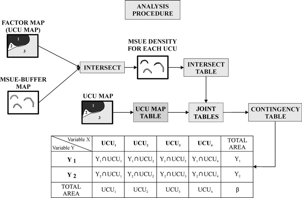
Procedure used in the Python program to build the contingency tables. A very simple case with only one landslide type is considered. See the text for a detailed explanation.
Based on the contingency table shown on Fig. 4, the Pearson's χ2 was defined as follows:
| (7) |
| (8) |
3.7 Multifactor analysis and best model statistical significance
In the GIS environment, all combinations of the landslide-related factors with slope aspect (UCU maps) were computed initially. Next, the UCU maps were intersected for each landslide type with the buffer maps of the MSUEs that belonged to the pre-1975 dataset. For each UCU, the ratio of the MSUE buffer area that falls within the UCU to the total area of the UCU was calculated (UCU density). In addition, the UCUs were grouped into five density classes that were based on the mean density of the UCU (Md) (Clerici et al., 2010), including 0–0.4Md (very low), 0.4–0.8Md (low), 0.8–1.2Md (medium), 1.2–1.6Md (high) and 1.6–2.0Md (very high).
The absolute difference between the pre- and post-1975 MSUE percentages was computed for each LS class in the validation procedure. The sum of the post-1975 MSUE percentages [the validation error (VE)] was reported for each LS model to assess the predictive power of each model. This value ranged from 0 (best predictive power) to 200 (worst).
According to Clerici et al. (2010), a good model should significantly disperse around the UCU mean density (high mean deviation of the UCU density) to distinguish the different probabilities of future landslides and to provide a spatially detailed forecast. Therefore, the mean deviation (MD) of the UCU density was computed for each model and the MD/VE ratio (the best model index, BMI) was used to choose the best LS model with the greatest BMI.
The reduced Chi2 (χ2) variable was determined to evaluate how the predictive ability of the best model represented the maximum likelihood between the landslide groups that were used for model construction and validation. The χ2 value for a model defines the probability of finding a likelihood between the observed and expected probabilities of a certain event A, which is better than that defined by the model itself (Buccianti et al., 2003; Kendall and Stuart, 1979; Pugh and Winslow, 1966). The forecasting model should be made from older landslide inventories. Recent landslide information should be used to evaluate the prediction power of the model (Blahut et al., 2010; Chung and Fabbri, 2008; von Ruette et al., 2011). For each model, the percentage of landslides belonging to the validation group that fall into a susceptibility class must be considered as an expected value of the landsliding probability in that class.
Therefore, in this study the Chi2 value was calculated as follows:
| (9) |
4 Results and discussion
Regarding the connection between landslides and slope aspect, the density values reported in Table 3 show non-negligible differentiation between the minimum and maximum for the translational and rotational slides of the Milia basin and for the flows and translational slides of the Roglio basin. For these types of landslides, greater density values are concentrated on the E–SW and NW-facing slopes. This trend is similar to trends that have been observed in recent LS studies that were performed at middle latitudes in the northern hemisphere (Bednarik et al., 2010; Magliuolo et al., 2008; Piacentini et al., 2012; Regmi et al., 2010; Yalcin, 2008; Yalcin et al., 2011). In these studies, the N–NW-facing slopes are favorable for landslides due to their shadier, colder, and more humid conditions. In contrast, the east–south-facing slopes are very prone to landslides because they are affected by intense wetting and drying cycles.
Independently of landslide typology, the Pearson's χ2 values for each basin showed a spatial correlation between the geo-environmental factors and the occurrence of landslides (with a confidence level of 0.01) (Table 4). The strength of the spatial associations between the geo-environmental factors and the landslides were quantified by the value of Cramer's V (Kendall and Stuart, 1979). As reported in Table 4, the lithology, slope angle, and distance to streams had the greatest values of Cramer's V for each landslide typology. This finding confirmed that these factors played a dominant role in controlling the spatial distributions of the landslides. However, the distance to the streams in the Roglio basin had a low value of Cramer's V for the rotational slides.
Spatial correlation degree between the landslides and the geo-environmental factors, for each landslide typology and for each basin studied. The Chi2 tests were performed with 99% confidence level.
| Roglio basin | ||||||
| Translational slide | Flow | Rotational slide | ||||
| χ 2 | V | χ 2 | V | χ 2 | V | |
| Lithology | 15,164 | 0.31 | 7163 | 0.26 | 735 | 0.15 |
| Slope angle | 27,110 | 0.36 | 3822 | 0.22 | 493 | 0.13 |
| Slope aspect | 1493 | 0.17 | 312 | 0.12 | 84 | 0.09 |
| Distance to tectonic elements | 225 | 0.10 | 1284 | 0.17 | 777 | 0.14 |
| Distance to streams | 4140 | 0.22 | 2843 | 0.20 | 354 | 0.12 |
| Milia basin | ||||||
| Translational slide | Flow | Rotational slide | ||||
| χ 2 | V | χ 2 | V | χ 2 | V | |
| Lithology | 12,551 | 0.33 | 1594 | 0.20 | 3654 | 0.25 |
| Slope angle | 2648 | 0.23 | 392 | 0.14 | 1281 | 0.19 |
| Slope aspect | 147 | 0.11 | 45 | 0.08 | 622 | 0.16 |
| Distance to tectonic elements | 706 | 0.16 | 219 | 0.12 | 342 | 0.13 |
| Distance to streams | 2297 | 0.22 | 960 | 0.18 | 1242 | 0.19 |
Regarding the slope aspect, the values of Cramer's V were spatially correlated with the translational and rotational slides of the Roglio and Milia basins, respectively. For these types of landslides, the Cramer's V values were comparable to the values obtained from the lithology and flows (Milia basin) and the lithology and rotational slides (Roglio basin).
The importance of slope aspect as a landslide-predisposing factor for translational slides in the Roglio basin potentially resulted from thermal excursions and the drying of clayey sediment (Pliocene deposits). The density values reported in Table 3 show a trend that is similar to the trend that was observed for the spatial distribution of the badlands (Fig. 2). The thermal excursions and drying action in the Pliocene deposits should only affect the superficial portion of the slope (Lulli and Ronchetti, 1973; Vittorini, 1977, 1979). In addition, the translational slides of the Roglio basin have a lower average size than the other types of landslides (Table 2). These facts indicate that slope aspect is an important predisposing factor for translational slides.
According to the modeled likelihood Chi2 test of the Roglio basin, if a P-value of P(χ2 < χ2 observed) < 0.05 is considered, the best LS model for the slope aspect and the other landslide-predisposing factor combinations (Table 5) is considered as the best overall model with a high level of statistical significance (Table 6). Thus, the hypothesis that slope aspect has conditioned the spatial distribution of translational landslides in the Roglio basin is accepted at the 95% confidence level.
The five best models of landslide susceptibility obtained for each basin and each landslide type ordered by decreasing best model index (BMI) values.
| Roglio basin | |||||||||||
| Translational slide | Flow | Rotational slide | |||||||||
| FC | VE | MD | BMI | FC | VE | MD | BMI | FC | VE | MD | BMI |
| ADiDf | 6.3 | 3629 | 576.0 | SADi | 11.0 | 2079 | 189.0 | LSADi | 138.0 | 1921 | 13.9 |
| LSADi | 29.2 | 14,140 | 484.2 | LADf | 11.8 | 2050 | 173.7 | LA | 65.2 | 881 | 13.5 |
| LADi | 25.2 | 11,244 | 440.9 | LSA | 11.3 | 1950 | 172.6 | LADiDf | 131.5 | 1083 | 8.2 |
| ADi | 5.5 | 2338 | 425.1 | LSADf | 14.1 | 2194 | 155.6 | LSADiDf | 174.0 | 1410 | 8.1 |
| LADiDf | 27.9 | 10,594 | 379.7 | LSADi | 22.5 | 3232 | 143.7 | LADf | 106.4 | 688 | 6.5 |
| Milia basin | |||||||||||
| Translational slide | Flow | Rotational slide | |||||||||
| FC | VE | MD | BMI | FC | VE | MD | BMI | FC | VE | MD | BMI |
| LSA | 11.7 | 10,489 | 896.5 | ADi | 12.9 | 643 | 49.8 | LADf | 42.5 | 2395 | 56.4 |
| LADi | 13.2 | 10,659 | 807.5 | ADiDf | 19.9 | 878 | 44.1 | LSA | 50.2 | 2224 | 44.3 |
| LA | 11.8 | 8780 | 744.1 | LADi | 27.2 | 1134 | 41.7 | LADiDf | 72.0 | 3150 | 43.8 |
| LADf | 16.0 | 9528 | 595.5 | LA | 24.5 | 961 | 39.2 | LSADf | 61.8 | 2684 | 43.4 |
| LSADi | 22.7 | 13,227 | 582.7 | SADi | 24.4 | 874 | 35.8 | LA | 48.7 | 2078 | 42.7 |
Chi2 statistics of the best models. The Chi2 tests were performed with four degree of freedom and 0.05 confidence level (χ2critic = 0.177).
| Roglio basin | Model | VE | χ2obs. | P(χ2 < χ2obs.) |
| Translational slides | ADiDf | 6.3 | 0.175 | < 0.05 |
| Flows | SADi | 11.0 | 0.615 | > 0.05 |
| Rotational slides | LSADi | 138.0 | 7.675 | > 0.05 |
| Milia basin | Model | VE | χ2obs. | P(χ2 < χ2obs.) |
| Translational slides | LSA | 11.7 | 0.422 | > 0.05 |
| Flows | ADi | 12.9 | 0.673 | > 0.05 |
| Rotational slides | LADf | 42.5 | 3.125 | > 0.05 |
Based on the bivariate analysis of the Milia basin, the role that the landslide rotational slide-predisposing factor plays is ambiguous. The rotational slides have a large average size (Table 2), which implies an average rupture surface that is too deep for determining the influences of shade and sun on their development. In addition, although the maximum rotational density values are concentrated on the NW-facing slopes (Table 3), it is difficult to prove that shadier, colder, or humid conditions affected the stability of the slope at depths of more than 10 m.
In the likelihood Chi2 test model of the Milia basin, the introduction of the slope aspect factor in the multifactor analysis did not maximize the likelihood of the best model until a high level of statistical significance (Table 6). Thus, the assertion that slope aspect has conditioned the spatial distribution of the rotational slide type landslides in the Milia basin cannot be accepted at a confidence level of 95%.
Based on the model likelihood Chi2 test results, slope aspect is a significant landslide-predisposing factor for the superficial landslides of the Roglio basin (i.e., translational slides).
When comparing the results obtained from the multifactor and bivariate analysis with the different studies that were performed over the last two decades (e.g., Blahut et al., 2010; Cevik and Topal, 2003; He et al., 2012; Komac, 2006; Van Den Eeckhaut et al., 2006; Yalcin et al., 2011), raises suspicion that only rarely slope aspect can be a landslide-predisposing factor. More detailed, slope aspect can be correlated with one or more of the geo-environmental factors that have really affected the landslide development, and that are usually not considered in the statistical analysis. Over the last decade, the statistical correlation between the slope aspect and other landslide-predisposing factors has been pointed out by some works (Regmi et al., 2010; Van Den Eeckhaut et al., 2009), whereas some studies postulated an influence of local factors on the evolution of slope aspect (Ayalew and Yamagishi, 2005; Fernandes et al., 2004; Gao and Maro, 2010; Ghosh et al., 2011). For example, Fernandes et al. (2004) determined how hillslope orientation is inherited from bedrock structure, especially metamorphic foliation. In the Milia basin, the fracture systems that were associated with the axial plane folds of the Ligurian formations potentially played an important role in the predisposition of rotational slides when the hydrographic network was rapid sinking. Because most of the higher order streams in the Milia basin were generated in the NE–SW direction, the occurrence of rotational slides on the NW-facing slopes supports the idea that the slope aspect is correlated with the Milia fracture systems. This correlation reveals an apparent landslide-predisposing power in the bivariate analysis. However, the fracture system study represents an analysis with a high cost/benefit value, which is generally not performed in the definition of an LS at the basin level (Soeters and van Westen, 1996; van Westen et al., 2008).
5 Conclusions
The general aim of this study was to highlight considerations that could be useful for understanding the roles played by slope aspect in predicting the spatial distribution of landslides. Slope aspect only functioned as a landslide-predisposing factor when the landslides were superficial and in clayey deposits. Conversely, a large value of Cramer's V did not indicate that slope aspect is a landslide-predisposing factor in the general case.
Previous and current results indicate the presence of a correlation between slope aspect and other (normally unconsidered) geo-environmental factors. This correlation may affect the actual weight of slope aspect as a landslide-predisposing factor, potentially leading to a wrong interpretation of the slope instability causes.
Acknowledgements
This research was supported by the Tuscany Region Project CIPE/Regione Toscana: Carta Geologica Regione Toscana e geo-tematiche derivate (Leaders Prof. P.R. Federici, Prof. A. Puccinelli), and the Italian MIUR Project (PRIN 2010–11): “Response of morphoclimatic system dynamics to global changes and related geomorphological hazards” (national and local coordinator Prof. C. Baroni). The authors would like to thank Prof. Aldo Clerici and Prof. Birgit Terhorst for their comments, which improved the paper. We would also like to acknowledge the professional English editing services of the American Journal Experts.