F-layer formation in the outer core with asymmetric inner core growth

Renaud Deguen; Peter Olson; Evan Reynolds

doi:10.1016/j.crte.2014.04.003

Internal geophysics

F-layer formation in the outer core with asymmetric inner core growth

Renaud Deguen ¹ ; Peter Olson ² ; Evan Reynolds ²

¹ LGL, Laboratoire de géologie de Lyon – terre, planète, environnement, CNRS, Université Lyon-1, Villeurbanne, France
² Department of Earth and Planetary Sciences, Johns Hopkins University, Baltimore, MD, USA

Comptes Rendus. Géoscience, Volume 346 (2014) no. 5-6, pp. 101-109.

Résumé

Numerical calculations of thermochemical convection in a rotating, electrically conducting fluid sphere with heterogeneous boundary conditions are used to model effects of asymmetric inner core growth. With heterogeneous inner core growth but no melting, outer core flow consists of intense convection where inner core buoyancy release is high, weak convection where inner core buoyancy release is low, and large scale, mostly westward flow in the form of spiraling gyres. With localized inner core melting, outer core flow includes a gravity current of dense fluid that spreads over the inner core boundary, analogous to the seismic F-layer. An analytical model for gravity currents on a sphere connects the structure of the dense layer to the distribution of inner core melting and solidification. Predictions for F-layer formation by asymmetric inner core growth include large-scale asymmetric gyres below the core-mantle boundary and eccentricity of the geomagnetic field.

Métadonnées

Reçu le : 2014-03-11
Accepté le : 2014-04-12
Publié le : 2014-05-01

DOI : 10.1016/j.crte.2014.04.003

Mots clés : Seismic F-layer, Inner core melting, Inner core translation, Geodynamo

Affiliations des auteurs :

Renaud Deguen ¹ ; Peter Olson ² ; Evan Reynolds ²

@article{CRGEOS_2014__346_5-6_101_0,
     author = {Renaud Deguen and Peter Olson and Evan Reynolds},
     title = {F-layer formation in the outer core with asymmetric inner core growth},
     journal = {Comptes Rendus. G\'eoscience},
     pages = {101--109},
     publisher = {Elsevier},
     volume = {346},
     number = {5-6},
     year = {2014},
     doi = {10.1016/j.crte.2014.04.003},
     language = {en},
}

TY  - JOUR
AU  - Renaud Deguen
AU  - Peter Olson
AU  - Evan Reynolds
TI  - F-layer formation in the outer core with asymmetric inner core growth
JO  - Comptes Rendus. Géoscience
PY  - 2014
SP  - 101
EP  - 109
VL  - 346
IS  - 5-6
PB  - Elsevier
DO  - 10.1016/j.crte.2014.04.003
LA  - en
ID  - CRGEOS_2014__346_5-6_101_0
ER  -

%0 Journal Article
%A Renaud Deguen
%A Peter Olson
%A Evan Reynolds
%T F-layer formation in the outer core with asymmetric inner core growth
%J Comptes Rendus. Géoscience
%D 2014
%P 101-109
%V 346
%N 5-6
%I Elsevier
%R 10.1016/j.crte.2014.04.003
%G en
%F CRGEOS_2014__346_5-6_101_0

Renaud Deguen; Peter Olson; Evan Reynolds. F-layer formation in the outer core with asymmetric inner core growth. Comptes Rendus. Géoscience, Volume 346 (2014) no. 5-6, pp. 101-109. doi : 10.1016/j.crte.2014.04.003. https://comptes-rendus.academie-sciences.fr/geoscience/articles/10.1016/j.crte.2014.04.003/

Version originale du texte intégral

1 Introduction

The seismic F-layer is defined by a decrease in the compression wave (P wave) velocity gradient in an approximately 150–200 km-thick layer in Earth's outer core located just above the inner core boundary (ICB). The anomalous gradient in this region is large enough that it has recently been incorporated into a number of global seismic models, as shown in Fig. 1. Most observations indicate that the F-layer is global, that is, it surrounds the entire inner core (Cormier, 2009; Cormier et al., 2011; Souriau and Poupinet, 1991; Zou et al., 2008), although lateral variations in its properties remain an open possibility (Yu et al., 2005).

Fig. 1
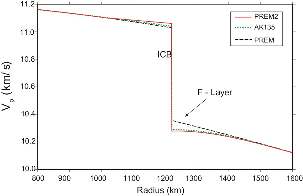
(Color online). Variation of compression wave velocity V_p versus radius through the core showing the anomalous F-layer at the base of the outer core, according to seismic models PREM (Dziewonski and Anderson, 1981), AK135 (Kennett et al., 1995), and PREM2 (Song and Helmberger, 1995); after Zhou et al. (2008). ICB denotes the inner core boundary.

Interpretations of the F-layer attribute its anomalous seismic velocity gradient to an approximately monotonic increase in the heavy element concentration (Fe and Ni) with depth, or equivalently, a corresponding decrease in the light element concentration (O, Si, S…) with depth at the base of the liquid outer core (Gubbins et al., 2008). An increase in iron content relative to light elements that accounts for the reduced P wave velocity gradient there has the opposite effect on outer core density (Badro et al., 2007), producing a density increase with depth, i.e., a stable compositional stratification.

The possibility of stable density stratification at the base of the outer core raises important questions about energy transfer and dynamics in the core. According to the standard model of core energetics (Labrosse, 2003), as the core cools, solidification at the ICB partitions heavy elements into the solid and lighter elements into the liquid, providing the primary source of buoyancy for driving convection in the liquid outer core. Under these conditions, the region above the ICB would be expected to have neutral or slightly unstable density stratification due to its elevated light element concentration. Adding a layer with stable stratification complicates this picture in several ways. First, it begs the question of how the F-layer formed. Second, it appears to limit the downward transport of light elements from the outer core to the ICB, thereby inhibiting compositional convection in the outer core.

Several mechanisms have been offered to explain the formation of the F-layer, each with far-reaching implications for the dynamics in the core. One possibility is that the F-layer is a relic of the core formation process. This mechanism is based on the idea that the light element abundances in core-forming metals evolved with time as the Earth accreted in such a way that the core was built with an initial radial stratification consisting of progressively less dense alloys (Hernlund et al., 2013). According to this scenario, the F-layer consists of the remnants of the initial stratification. Another proposal is that the F-layer is maintained by iron solidifying at the top of the layer then re-melting as it precipitates through the layer (Gubbins et al., 2008).

By far the most provocative mechanism, and the one we focus on in this study, assumes that the F-layer is maintained through the interaction of separated melting and solidifying regions distributed over the ICB (Alboussière et al., 2010). Because the ICB is a phase change boundary, substantial lateral variations in temperature must be present there for melting and freezing to occur simultaneously. The core-mantle boundary (CMB) is one possible source of these lateral temperature variations. Experiments (Sumita and Olson, 1999, 2002) and numerical simulations (Aubert et al., 2008) have shown that temperature anomalies generated by strongly heterogeneous CMB heat flux can be transmitted from the CMB to the ICB by outer core convection. Gubbins et al. (2011) demonstrated that, under proper conditions, these CMB-generated temperature anomalies can produce a pattern of simultaneous melting and freezing on the ICB.

The other possibility is convection in the solid inner core. The simplest form of inner core convection consists of melting and solidification in separate hemispheres, leading to a lateral translation of the solid material in the inner core from the freezing hemisphere to the melting one, the so-called inner core translation mode (Alboussière et al., 2010; Monnereau et al., 2010). In addition to the substantial interest in its energetics and dynamics, inner core translation offers a plausible explanation for the observed east–west variations in seismic anisotropy in the inner core (Bergman et al., 2010; Deuss et al., 2010; Niu and Wen, 2001; Sun and Song, 2008; Tanaka and Hamaguchi, 1997), thereby linking its seismic structure to its growth.

The onset of subsolidus convective instabilities in the inner core, including the translational mode, has been examined using several approaches (Buffett, 2009; Cottaar and Buffett, 2012; Deguen and Cardin, 2011; Deguen et al., 2013; Jeanloz and Wenk, 1988; Mizzon and Monnereau, 2013; Weber and Machetel, 1992). The main requirement for convective instability in the inner core is an adverse radial density gradient. Inner core translation is the preferred mode of instability at high viscosity, as it involves little or no solid-state deformation. Cellular (i.e., higher mode) convection favored at viscosities less than about 310¹⁸ Pa.s can also produce localized melting and solidification, but less efficiently than the translation mode (Deguen et al., 2013; Mizzon and Monnereau, 2013).

A systematic investigation of the influence of inner core translation on the outer core by Davies et al. (2013) examined thermal convection driven by a spherical harmonic degree and order one pattern of heat flux applied at the ICB. They found that the flow transitions from the usual columnar-style convection when the ICB is homogeneous (Sumita and Olson, 2000) to a pattern dominated by larger-scale mostly prograde (eastward) spiraling jets when the ICB heterogeneity is strong. In cases where the ICB heterogeneity was large enough to simulate melting (corresponding to negative ICB heat flux in their model) the spiral jets found by Davies et al. (2013) resulted in large hemispherical differences in azimuthal velocity everywhere in the outer core, including below the CMB.

Several previous studies have examined dynamo action with spherical harmonic degree one ICB heterogeneity. Results of these studies include dipole eccentricity (Olson and Deguen, 2012) as well as east-west asymmetry in the secular variation of the magnetic field (Aubert, 2013; Aubert et al., 2013). Aubert et al. (2013) have shown that the differences in the geomagnetic secular variation observed between Atlantic and Pacific hemispheres can be produced by a relatively small amount of hemispherically asymmetric inner core buoyancy flux, provided it is properly oriented. In particular, they found that the observed asymmetry of the geomagnetic secular variation is best explained if the buoyancy flux is maximum in the eastern hemisphere, implying westward inner core translation, which is the opposite direction from the original interpretations of the inner core anisotropy (Bergman et al., 2010; Geballe et al., 2013; Monnereau et al., 2010), though in agreement with other interpretations of the observed seismic properties of the inner core (Cormier and Attanayake, 2013; Cormier et al., 2011).

In this study we consider the effects of asymmetric inner core growth including translation in the context of thermochemical convection and dynamo action, using hemispheric variations of codensity at the ICB to represent inner core melting and solidification. First we use numerical simulations of rotating non-magnetic convection to examine the changes in flow and stratification in the outer core that accompany increasing amounts of this type of codensity heterogeneity. We then consider these effects on the geomagnetic field using numerical dynamos that include hemispherical inner core codensity variations. Lastly, we derive an analytical gravity current model for interpreting our numerical simulations and relating them to the observed F-layer structure.

2 Thermochemical convection with hemispherical inner core growth

To model the effects of hemispherically asymmetric inner core growth including melting and solidification on the ICB, we define codensity C in the outer core as the sum of temperature and light element concentration,

C = ρ_{0} (α T + β χ)

(1)

where ρ₀ is average density, T is temperature relative to the adiabat, χ is light element concentration (mixing ratio), and α and β are volumetric expansion for T and χ, respectively. Let

{\dot{χ}}_{o}

denote the time rate-of-change of the volume-average mixing ratio on the outer core, assumed to be constant, and let v and κ denote outer core kinematic viscosity and diffusivity, respectively. Further, let Ω denote angular velocity of Earth's rotation, g denote gravity and D = r_o – r_i denote the depth of the outer core, r_o and r_i being the radii of the CMB and the ICB, respectively. In dimensionless form, the equations for conservation of momentum including rotation, conservation of mass, and codensity transport with the Boussinesq approximation in a rotating spherical shell (Jones, 2007) contain the following dimensionless control parameters:

E = \frac{ν}{Ω D^{2}}, \Pr = \frac{ν}{κ}, R a = \frac{β g D^{5} {\dot{χ}}_{o}}{ν^{2} κ}

(2)

where E is the Ekman number, Pr is the Prandtl number, and Ra is the Rayleigh number. Here we have used D, D²/v and

ρ_{0} β D^{2} {\dot{χ}}_{o} / ν

to scale length, time, and codensity, respectively. An additional control parameter is the volumetric codensity sink ɛ representing the absorption of buoyancy in the outer core.

At the CMB we assume no-slip velocity conditions and a uniform positive (destabilizing) codensity flux F₀, so that

F_{o} = - κ {\frac{\partial C}{\partial r}|}_{r = r_{o}},

(3)

with $F_{o}^{*}$ denoting the dimensionless version of (3). At the ICB, we assume no-slip velocity conditions and we specify a distribution of codensity modeling the combination of uniform plus heterogeneous inner core growth. Specifically, we set

C |_{r = r_{i}} = \bar{C} + C^{'}

(4)

where $\bar{C}$ and C′(θ, ϕ) are the mean and laterally varying codensity at the ICB, θ and ϕ denoting colatitude and longitude, respectively. To represent hemispherical ICB melting and solidification, we set

C^{'} = Δ C Y_{1,1} (θ, ϕ)

(5)

where ΔC is the amplitude of the ICB heterogeneity and Y_1,1 is a spherical harmonic of order and degree one. The ICB heterogeneity is symmetric about an axis defined by the points (θ = π/2, ϕ = π/2) and (θ = π/2, ϕ = 3π/2). In what follows, we call the point (θ = π/2, ϕ = π/2) where C′ is maximum the solidification pole and we call the point (θ = π/2, ϕ = 3π/2) the melting pole if C′ is negative there.

We can now define additional dimensionless parameters to characterize the ICB heterogeneity. One new control parameter is a lateral Rayleigh number based on the amplitude of the ICB codensity heterogeneity:

R a^{*} = \frac{β g D^{3} Δ C}{ν κ} .

(6)

A parameter that measures the system response to ICB heterogeneity is the buoyancy flux ratio, $ℛ^{*}$ . Using the codensity flux at the ICB

F_{i} (θ, ϕ) = - κ {\frac{\partial C}{\partial r}|}_{r = r_{i}}

(7)

the buoyancy flux ratio can be defined as

ℛ^{*} = \frac{\int_{ICB} F_{i}^{-} d A}{\int_{ICB} F_{i}^{+} d A}

(8)

where $F_{i}^{-}$ and $F_{i}^{+}$ denote the negative and positive F_i-values and the integrals are evaluated over the ICB area. The ratios Ra^*/Ra and $ℛ^{*}$ parameterize the extent of melting regions versus solidification regions on the ICB. For large values of these ratios, melting and solidification each cover approximately one-half of the ICB. For intermediate values, the melting region is finite but covers less than one-half of the ICB. For small values of Ra^*/Ra or for $ℛ^{*} = 0$ , (4) is positive everywhere on the ICB and there is no melting. Cases with small values of Ra^*/Ra with positive codensity everywhere on the ICB are meant to simulate uneven growth of the inner core that is subcritical to the translation instability. In the other extreme, cases with very large Ra^*/Ra are meant to simulate the effects of the translation instability.

3 Non-magnetic thermochemical convection with ICB heterogeneity

We have carried out two sets of non-magnetic thermochemical convection calculations using the MAGIC code (Wicht, 2002) with Y_1,1-type ICB conditions, varying the parameters Ra and Ra^*. Fig. 2 shows the resulting structure of the convection in the equatorial plane at E = 3 × 10⁻⁵ and Pr = 1 from calculations with numerical resolution (n_r, n_θ, n_ϕ) = (129, 192, 384). From top to bottom, the images show the effects of increasing amounts of ICB heterogeneity, represented by increasing values of the ratio Ra^*/Ra. The first three columns in Fig. 2 are snapshots of codensity, axial (z-component) vorticity, and azimuthal (ϕ-component) of velocity; the last column is the time average of the streamfunction of the flow.

Fig. 2
(Color online). Equatorial sections of rotating convection with hemispherical variation of codensity (Y_1,1-type heterogeneity) on the inner core boundary. From left to right, images show codensity, z-component of vorticity, azimuthal velocity v_ϕ, and the streamfunction of the motion. The streamfunctions are time averages, whereas the other images are snapshots in time. Rows 1–3 show the effects of increasing inner core heterogeneity (increasing heterogeneity Rayleigh number Ra^* with Ra fixed). Row 4 shows the effects of inner core heterogeneity with zero codensity flux at the core-mantle boundary and Ra = 0. E = 3 × 10⁻⁵ and Pr = 1 in all cases. In each section the melting pole is on the left, the solidification pole is on the right, the solid line marks the melting equator, and the gray shading indicates inner core age increasing from light to dark.

The top row of images in Fig. 2 show a moderate amount of hemispherical asymmetry in all variables at Ra^*/Ra = 0.125. Since F_i is positive over the entire ICB in this calculation, there is no melting implied and nothing that would correspond to the F-layer. Nevertheless, convection is substantially more vigorous above the ICB in the hemisphere where C′ > 0. The azimuthal velocities are primarily retrograde (westward), are highest near the solidification pole and near the CMB there is a broad velocity minimum (CMB quiet zone) about 90° east of the solidification pole.

The two middle rows in Fig. 2 show the effects of increasing ICB heterogeneity including regions with F_i < 0, analogous to melting. At Ra^*/Ra = 0.25 (2nd row in Fig. 2) the hemispherical differences are magnified compared to the Ra^*/Ra = 0.125 case, and a thin spherical cap with positive codensity gradient (negative codensity flux) is clearly evident above the ICB in the hemisphere where C′ < 0. Convection above this stably stratified cap is noticeably attenuated, and the vorticity pattern in the cap indicates the presence of a thin gravity current just above the ICB. In addition, the region with the most intense convection and the CMB quiet zone are both shifted farther to the west. These effects are amplified in the Ra^*/Ra = 0.5 case shown in the third row of Fig. 2, where the high density gravity current covers more than half of the ICB and the CMB quiet zone is located almost directly above the solidification pole. In the extreme case with Ra^* finite and $R a = ε = F_{o}^{*} = 0$ shown in the bottom row of Fig. 2, the convection is maintained by ICB heterogeneity alone, the gravity current covers most of the ICB, convection is restricted to a localized region, and the CMB quiet zone has been shifted west of the solidification pole.

The winding of the spiral in the azimuthal flow with increasing Ra^*/Ra is most evident in the time average streamfunction in Fig. 2, as the longitude of the CMB quiet zone shifts progressively westward. The tendency for spiral tightening with increasing Ra^* and decreasing E was first reported by Davies et al. (2013). Interestingly, however, the direction of the dominant azimuthal flow in the equatorial plane of their calculations is prograde (eastward), possibly because they model thermal convection, whereas our convection is primarily compositional. Our azimuthal flows also differ somewhat from the azimuthal flows reported by Aubert (2013) who used heterogeneous codensity flux conditions on the ICB (rather than the heterogeneous codensity ICB conditions we use) and found a prograde and a retrograde spiral jet of nearly equal strength. In light of these differences, it is clear that the large-scale azimuthal flows are sensitive to the choice of boundary conditions and the type of convective forcing assumed, not to mention external factors such as angular momentum exchange with the mantle.

Nevertheless, there are qualitative similarities between our azimuthal flow patterns and the generally westward flow in the equatorial plane of the outer core inferred by Pais and Jault (2008) and Gillet et al. (2009) from the geomagnetic secular variation. Based on the location of the CMB quiet zone, the Ra^*/Ra = 0.125 case in Fig. 2 is closest to the model preferred by Aubert et al. (2013) for explaining asymmetry in the geomagnetic secular variation, which would imply no ICB melting.

We have made a second set of non-magnetic calculations in order to determine the minimum amount of melting needed to produce the F-layer. Fig. 3 shows the correlation of the time average $ℛ^{*}$ versus Ra^* from 13 cases at E = 10⁻⁴ and various Ra^*-values. The inset shows the criterion used to identify stable stratification, namely, a sign reversal in the average codensity gradient above the ICB. Filled and open symbols denote the presence or absence of an F-layer according to this prescription. Although there is considerable scatter, the results in Fig. 3 are consistent with the interpretation that a certain minimum amount of melting, corresponding to $ℛ^{*} ≃ 0.25$ , is needed for a stable layer to form.

Fig. 3
(Color online). F-layer regime diagram in terms of inner core buoyancy flux ratio $ℛ^{*}$ versus Rayleigh Number Ra for rotating convection with Y_1,1-type codensity heterogeneity on the inner core boundary. Criterion of F-layer formation is the presence of a reverse codensity gradient as shown in the insert. Solid symbols with F-layer, open symbols without. Dashed line denotes the approximate boundary between these two regimes.

4 Dynamo action with inner core melting

The previous studies of dynamo action with hemispheric inner core growth imposed relatively modest ICB heterogeneity, generally too small in amplitude to produce negative buoyancy flux and therefore too small to simulate inner core melting. Accordingly, we consider here the influence of large amplitude ICB heterogeneity, as would produce an extensive melting region on the ICB.

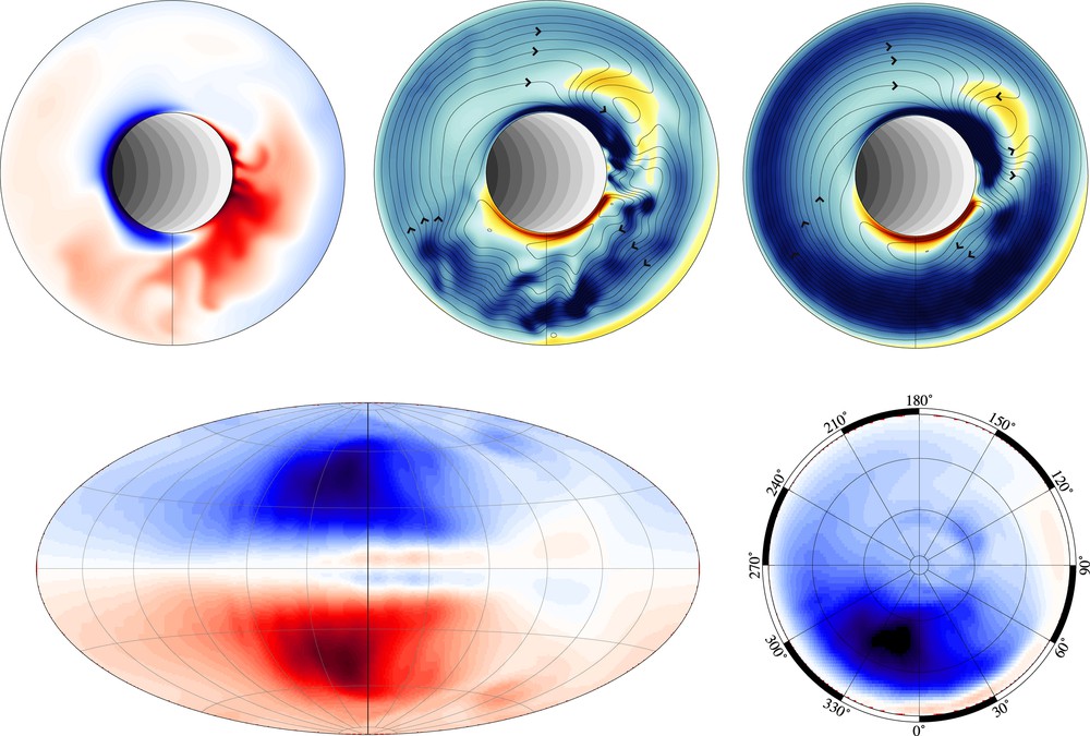
Fig. 4 shows the structure of a numerical dynamo with Ra = 4 × 10⁶, Ra^* = 2.3 ×10⁷, $F_{o}^{*} = 0$ , E = 10⁻⁴, ɛ = –1 along with Pr = Pm = 1, where Pm is the magnetic Prandtl number. The upper row of equatorial plane images are, from left to right, a snapshot of the codensity, and the corresponding snapshot of the streamfunction with z-vorticity contours, and the time average of the streamfunction with z-vorticity contours. As with previous equatorial sections, the melting pole is on the left, the solidification pole is on the right, the solid line marks the melting equator, and the gray shading indicates inner core age increasing from light to dark. The lower row shows the time average of the radial magnetic field on the CMB and a polar view of the radial magnetic field on the CMB.

Fig. 4
(Color online.) Dynamo structure with hemispherical asymmetric inner core growth. Numerical parameters are given in the text. Top images are snapshot of the codensity in the equatorial plane (left); snapshot of the streamfunction and axial (z-component) vorticity contours in the equatorial plane (middle); and time averages of the streamfunction and axial vorticity contours in the equatorial plane (right). In the equatorial sections the melting pole is on the left, the solidification pole is on the right, the solid line marks the melting equator, and the gray shading indicates inner core age increasing from light to dark. Bottom images are time average radial magnetic field on the CMB (left) and north polar view of the radial magnetic field on the CMB (right).

For this dynamo, Ra^*/Ra is large, corresponding to rapid translation, melting is extensive, and the influence of ICB heterogeneity is pervasive. The codensity pattern in the outer core in Fig. 4 reflects the hemispherical ICB codensity pattern, but in this case the contrast between the stable cap on the melting side and the fine scale convection near the solidification pole is particularly evident, and highlights the contrasting dynamics in stable versus unstable regions.

Streamlines in the snapshot and time average images show predominantly westward azimuthal flow throughout most of the outer core, with the CMB quiet zone lying slightly west of the solidification pole, as was found for large Ra^* non-magnetic convection. Note the presence of a stagnation point in the snapshot and time average streamline patterns just above the melting pole, marking the center of divergent flow in the dense layer above the ICB, with westward flow to its west and eastward flow to its east. The location of this streamline divergence marks the center of the dense gravity current that in this case extends past the melting equator, covering nearly 80% of the ICB.

The magnetic field structure shows more radial coherence than the azimuthal velocity. Fig. 4 shows the high intensity field is shifted westward by about 90° at the CMB with respect to the solidification pole. More significantly, the dipole axis is offset from the rotation axis. The best-fitting dipole axis, determined using the method of James and Winch (1967), has virtually zero tilt in this case, a consequence of the north-south mirror symmetry in the large-scale magnetic field. However, the best-fitting dipole axis is offset from the center by a distance equal to 0.2r_o in the general direction of the inner core melting equator, to the west of the solidification pole and to the east of the melting pole. In terms of offset direction, this is qualitatively consistent with the findings of Olson and Deguen (2012), although the westward shifts of the dipole axes they found were generally smaller than shown here, differences can be attributed to differences in dynamo model parameters and boundary conditions.

5 Gravity currents in the F-layer

Figs. 2 and 4 indicate that formation of the F-layer by a heterogeneous distribution of melting and solidification on the ICB can be conceptualized in terms of a thin gravity current spreading slowly over a spherical surface, subject to a heterogeneous influx of mass representing inner core melting and solidification.

To model these dynamics, we assume the density anomaly in the F-layer decreases linearly with distance above the ICB according to

δ ρ = Δ ρ (1 - z / h)

(9)

where Δρ is the (positive) density anomaly at the ICB, z is radial distance above the ICB, and h is the anomalous layer thickness. Let u denote the z-averaged fluid velocity tangent to the ICB in the F-layer. Neglecting inertial and rotation effects, the equation of motion for the F-layer can be written as the following force balance:

g^{'} \nabla h = - k u

(10)

where k is the friction coefficient,

g^{'} = g_{0} Δ ρ / 3 ρ_{0}

is the effective (negative) buoyancy in the F-layer associated with the density profile (9), and g₀ and ρ₀ denote the mean values of gravity and density in the layer, which is assumed thin, i.e. h/r_i << 1.

The particular form of the friction coefficient depends on the mechanism of resistance to flow in the layer. Resistance to flow from the geomagnetic field is likely to be most important in Earth's electrically conducting core, whereas viscosity resists the flow in our non-magnetic convection calculations. In general, the friction coefficient can be written as a sum of these two effects:

k = k_{σ} + k_{ν} .

(11)

Resistance to flow in the layer from the Lorentz force due to a uniform radial magnetic field with intensity B₀ yields

k_{σ} = \frac{σ B_{0}^{2}}{ρ_{0}}

(12)

in which σ is electrical conductivity, whereas flow resistance due to uniform viscosity in the layer with a no-slip lower and a free-slip upper boundary yields

k_{ν} = \frac{40}{11} \frac{ν}{h^{2}}

(13)

where v is kinematic viscosity. In what follows, we first consider a gravity current with

k = k_{σ}

for application to Earth's core, then we consider a gravity current with k = k_v for interpreting our non-magnetic convection calculations.

Assuming incompressible flow, conservation of mass for the layer can be written as

\frac{\partial h}{\partial t} + \nabla \cdot (u h) = 2 w

(14)

where t is time and w is the volume flux per unit area into the layer from the inner core. Positive w corresponds to a mass flux into the layer with magnitude Δρw, i.e., inner core melting, whereas negative w corresponds to a mass flux out of the layer, i.e., inner core solidification. The factor 2 appears on the r.h.s. of (14) because of the assumed linear variation of anomalous density in the layer given by (9). Combining (10) and (14) yields the following equation for the evolution of the gravity current layer thickness h:

\frac{\partial h}{\partial t} - \frac{g^{'}}{2 k_{σ}} \nabla^{2} h^{2} = 2 w

(15)

where ▿² denotes the Laplacian on the spherical surface r = r_i. Analytical steady-state solutions to (15) can be obtained by expanding the source-sink function w and the squared layer thickness h² in terms of spherical harmonics Y_l,m:

w (θ, ϕ) = \sum_{l = 1}^{\infty} \sum_{m = - l}^{l} W_{l, m} Y_{l, m} (θ, ϕ)

(16)

and

h^{2} (θ, ϕ) = \sum_{l = 0}^{\infty} \sum_{m = - l}^{l} H_{l, m}^{2} Y_{l, m} (θ, ϕ)

(17)

where W_l,m and H²_l,m are the amplitudes of individual source-sink and layer thickness harmonics, respectively. Substituting (16) and (17) into (15) and ignoring time dependence yields

H_{l, m}^{2} = \frac{4 k_{σ} r_{i}^{2}}{g^{'}} \frac{W_{l, m}}{l (l + 1)}, l > 0

(18)

with the mean (spherically averaged) layer thickness H_0,0 being arbitrary in (17) by virtue of the steady-state assumption. To determine H_0,0 it would be necessary to assume an initial layer thickness and time integrate the unsteady gravity current equation (15). The steady-state results (18) predict a linear relationship between spherical harmonics of the melting/solidification pattern and spherical harmonics of the squared thickness of the F-layer. The factor in the denominator of (18) indicates that F-layer heterogeneity is most sensitive to the l = 1 (i.e., hemispherical) pattern of inner core melting/solidification.

The inner core translation hypothesis generally assumes that the melting and solidification poles lie in the equatorial plane, in the simplest case, 180° apart in longitude. Suppose the melting pole is located at (θ_m = π/2, ϕ_m), the solidification pole is located at (θ_s = π/2, ϕ_s = ϕ_m + π), and the melting/solidification pattern is symmetric about the the axis defined by these two poles. If λ denotes the great circle angular distance from the melting pole, then according to (17) and (18),

h^{2} (λ) = H_{0}^{2} + \frac{4 k_{σ} r_{i}^{2}}{g^{'}} \sum_{l = 1}^{\infty} \frac{W_{l, 0}}{l (l + 1)} Y_{l, 0} (λ),

(19)

which reduces to, for the case of pure inner core translation

h^{2} = h_{0}^{2} + \frac{2 k_{σ} r_{i}^{2} W}{g^{'}} (\cos λ - 1)

(20)

where h₀ is the layer thickness at the melting pole λ = 0 and we have used the abbreviation W = W_1,0 for the inner core translation speed.

The seismic observations argue for a global F-layer, formed by a dense stably stratified fluid enveloping the entire inner core, including the solidifying regions. In the context of our gravity current model, the transition from partial coverage to full inner core coverage is defined by the condition h² = 0 at λ = π. According to (20), the thickness of a global layer at its melting pole λ = 0 must therefore satisfy

h_{0} \geq \sqrt{\frac{4 k_{σ} r_{i}^{2} W}{g^{'}}} .

(21)

Assuming σ = 10⁶ S/m, B₀ = 10⁻³ T, and ρ₀ = 1.2 × 10⁴ kg/m³ implies $k_{σ} ≃ 10^{- 4} s^{- 1}$ in the F-layer. Using g′ = 0.03 m²/s and assuming W = 3 × 10⁻¹⁰ m/s (equivalent to a 300-Myr inner core translation time), the critical value of h₀ based on the r.h.s. of (21) is of the order of ten meters. Even this might be an overestimate, since we have ignored the possibility of magnetic flux expulsion from the gravity current. Indeed, the seismically observed F-layer thickness greatly exceeds the minimum thickness needed for full coverage of the ICB for any plausible combination of core properties, which is consistent with its inferred global structure.

When the flow resistance is due to viscosity, as in our non-magnetic convection calculations, the friction coefficient k_v defined by (13) depends on the layer thickness h and the structure of the gravity current is slightly different than derived above assuming magnetic field resistance. For a viscous gravity current, the analog equation to (15) for the evolution of the layer thickness is

\frac{\partial h}{\partial t} - \frac{c g^{'}}{ν} \nabla^{2} h^{4} = 2 w,

(22)

where c = 33/480. In terms of the expansions (16) and (17), the spherical harmonic coefficients of the viscous layer thickness in steady-state are given by

H_{l, m}^{4} = \frac{2 v r_{i}^{2}}{c g^{'}} \frac{W_{l, m}}{l (l + 1)}, l > 0 .

(23)

For purely hemispherical melting/solidification, the layer thickness varies over the ICB according to

h^{4} = h_{0}^{4} + \frac{ν r_{i}^{2} W}{c g^{'}} (\cos λ - 1),

(24)

which can be written in terms of the non-dimensionalization used in our non-magnetic convection calculations as

h^{* 4} = h_{0}^{* 4} + \frac{r_{i}^{* 2}}{c h_{0}^{*} R a^{*}} (\cos λ - 1) .

(25)

We can use (25) to calculate the relationship between the angular coverage by the gravity current and its dimensionless thickness at the melting pole. For partial coverage, these parameters are related by

h_{0}^{* 5} = \frac{r_{i}^{* 2}}{c R a^{*}} (1 - \cos λ_{\max}),

(26)

in which λ_max marks the leading edge of the gravity current where h^* = 0.

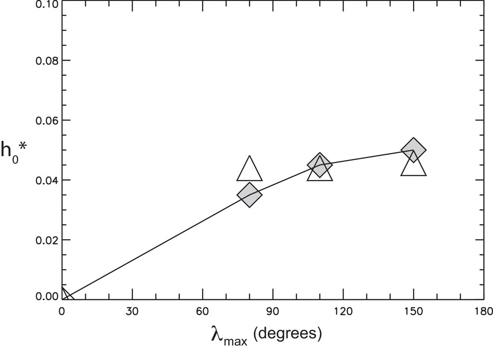
Fig. 5 shows the relationship between the angular coverage λ_max and melting pole thickness $h_{0}^{*}$ from the non-magnetic convection calculations shown in Fig. 2 compared to the gravity current model predictions using (26). The angular coverage in the convection calculations is defined as the average great circle distance at which the stable stratification vanishes, and the melting pole thickness is estimated using a straight line fit to the codensity profile there.

Fig. 5
Dimensionless gravity current layer thickness at the melting pole versus angular coverage of the ICB in degrees. Diamonds are determined from the non-magnetic convection calculations, triangles are predictions from the gravity current model.

Considering the various sources of error in these estimates, along with the highly idealized gravity current model, the rather small discrepancy in Fig. 5 is reassuring, although perhaps fortuitous. In particular, the stable layer thickness in the convection calculations is expected to differ from theoretical predictions because diffusion and entrainment effects, both of which tend to disperse the dense layer, are present in the convection calculations but are ignored in the gravity current model. Calculations with greater F-layer coverage have more extensive stably stratified regions where entrainment is presumably weak, whereas cases with less F-layer coverage have weaker, less extensive stratified regions and therefore are more prone to entrainment. Accordingly, cases with limited F-layers are more eroded relative to the non-entraining gravity current model. Finally, it needs to be emphasized that although the relative thicknesses h^* of the stable layer in our convection calculations are comparable to the observed thickness of the seismic F-layer relative to the outer core depth r_o – r_i, this is probably another fortuitous coincidence that results from the choice of the diffusivity in our convection models, which is far larger than appropriate for Earth's core.

6 Conclusions

Our calculations show that asymmetric release of buoyancy at the inner core boundary related to asymmetric inner core growth produces local and global perturbations in the core and the geomagnetic field. Moderately asymmetric inner core growth without melting produces moderate asymmetry in the core flow. In contrast, strongly asymmetric inner core growth with extensive melting, as would accompany rapid inner core translation, produces global-scale asymmetry in the core flow, and a highly eccentric magnetic field structure, perturbations that would be readily observable in the geomagnetic field, its secular variation, and probably also in the paleomagnetic field. The asymmetric structure of our numerical dynamo best conforms to the present-day dipole offset direction and the relatively quiet Pacific geomagnetic secular variation if the central longitude in Fig. 4 approximately corresponds to 180^* in the core, which would imply inner core translation from the western to the eastern hemisphere. However, this interpretation rests on very shaky ground, because the observed offset of the geomagnetic dipole is known to be time variable (Olson and Deguen, 2012) and because the longitude shifts in our models depend sensitively on poorly constrained core properties.

Inner core melting, represented in this study by negative buoyancy flux at the ICB, leads to formation of a stably stratified region above portions of the ICB, analogous to the seismic F-layer. Unlike the observed F-layer, the stable layers in our numerical calculations never entirely envelop the inner core, although they cover much of it in our most extreme cases. Our gravity current model explains this discrepancy in terms of the unrealistically high flow resistance in the numerical calculations, compared to the flow resistance expected in the outer core.

Lastly, we speculate that full coverage of the inner core by the F-layer as inferred seismically and predicted theoretically on the basis of its thickness presents conceptual problems for the long-term maintenance of the geodynamo via inner core growth. Full F-layer coverage is expected to inhibit the inward transport of light elements from the outer core to the ICB, meanwhile permitting their outward escape. Consequently, it is possible that over time the F-layer will so restrict the resupply of light elements to the ICB that the compositional buoyancy force in the outer core diminishes. Resupply of light elements could take place if portions of the ICB remain uncovered, or if the stable layer somehow remains permeable to their inward transport. Otherwise, the F-layer could eventually starve the outer core of its main source of power for convection.

Disclosure of interest

The authors declare that they have no conflicts of interest concerning this article.

Acknowledgments

This research was supported by Frontiers in Earth System Dynamics grant EAR-1135382 from the U.S. National Science Foundation.

Bibliographie

[Alboussière et al., 2010] T. Alboussière; R. Deguen; M. Melzani Melting-induced stratification above the Earth's inner core due to convective translation, Nature, Volume 466 (2010), pp. 744-747

[Aubert, 2013] J. Aubert Flow throughout Earth's core inverted from geomagnetic observations and numerical dynamo models, Geophys. J. Int., Volume 92 (2013) no. 2, pp. 537-556

[Aubert et al., 2008] J. Aubert; H. Amit; G. Hulot; P. Olson Thermo-chemical wind flows couple Earth's inner core growth to mantle heterogeneity, Nature, Volume 454 (2008), pp. 758-762

[Aubert et al., 2013] J. Aubert; C.C. Finlay; A. Fournier Bottom-up control of geomagnetic secular variation by the Earth's inner core, Nature, Volume 502 (2013) no. 7470, pp. 219-223

[Badro et al., 2007] J. Badro; G. Fiquet; F. Guyot; E. Gregoryanz; F. Occelli; D. Antonangeli; M. D’Astuto Effect of light elements on the sound velocities in solid iron: Implications for the composition of Earth's core, Earth Planet. Sci. Lett., Volume 254 (2007), pp. 233-238

[Bergman et al., 2010] M.I. Bergman; D.J. Lewis; I.H. Mying; L. Slivka; S.-I. Karato; A. Abreu Grain growth and loss of texture during annealing of alloys, and the translation of Earth's inner core, Geophys. Res. Lett., Volume 37 (2010), p. L22313

[Buffett, 2009] B. Buffett Onset and orientation of convection in the inner core, Geophys. J. Int., Volume 179 (2009), pp. 711-719

[Cormier, 2009] V.F. Cormier A glassy lowermost outer core, Geophys. J. Int., Volume 179 (2009), pp. 374-380

[Cormier et al., 2011] V.F. Cormier; J. Attanayake; K. He Inner core freezing and melting: constraints from seismic body waves, Phys. Earth Planet. Inter., Volume 188 (2011), pp. 163-172

[Cormier and Attanayake, 2013] V.F. Cormier; J. Attanayake Earth's solid inner core: seismic implications of freezing and melting, J. Earth Sci., Volume 24 (2013) no. 5.

[Cottaar and Buffett, 2012] S. Cottaar; B. Buffett Convection in the Earth's inner core, Phys. Earth Planet. Inter., Volume 198–199 (2012), pp. 67-78

[Davies et al., 2013] C.J. Davies; L. Silva; J. Mound On the influence of a translating inner core in models of outer core convection, Phys. Earth Planet. Inter., Volume 214 (2013), pp. 104-114

[Deguen and Cardin, 2011] R. Deguen; P. Cardin Thermochemical convection in Earth's inner core, Gephys. J. Int., Volume 187 (2011), pp. 1101-1118

[Deguen et al., 2013] R. Deguen; T. Alboussière; P. Cardin Thermal convection in Earth's inner core with phase change at its boundary, Gephys. J. Int., Volume 194 (2013) no. 3, pp. 1310-1334

[Deuss et al., 2010] A. Deuss; J. Irving; J. Woodhouse Regional variation of inner core anisotropy from seismic normal mode observations, Science, Volume 328 (2010), pp. 1018-1020

[Dziewonski and Anderson, 1981] A.M. Dziewonski; D.L. Anderson Preliminary Reference Earth Model, Phys. Earth Planet. Inter, Volume 25 (1981), pp. 297-356

[Geballe et al., 2013] Z.M. Geballe; M. Lasbleis; V.F. Cormier; E.A. Day Sharp hemisphere boundaries in a translating inner core, Geophys. Res. Lett., Volume 40 (2013), pp. 1719-1723

[Gillet et al., 2009] N. Gillet; M.A. Pais; D. Jault Ensemble inversion of time-dependent core flow models. Geochem, Geophys. Geosys., Volume 10 (2009) (6004D+)

[Gubbins et al., 2008] D. Gubbins; G. Masters; F. Nimmo A thermochemical boundary layer at the base of Earth's outer core and independent estimate of core heat flux, Geophys. J. Int., Volume 174 (2008), pp. 1007-1018

[Gubbins et al., 2011] D. Gubbins; B. Sreenivasan; J. Mound; S. Rost Melting of the Earth's inner core, Nature, Volume 473 (2011), pp. 361-363

[Hernlund et al., 2013] J. Hernlund; D.C. Rubie; S. Labrosse Primordial Stratification of the Earth's Core. Fall AGU abstract, 2013

[James and Winch, 1967] R.W. James; D.E. Winch The eccentric dipole, Pure Appl. Geophys., Volume 66 (1967), pp. 77-86

[Jeanloz and Wenk, 1988] R. Jeanloz; H.-R. Wenk Convection and anisotropy of the inner core, Geophys. Res. Lett., Volume 15 (1988), pp. 72-75

[Jones, 2007] C.A. Jones (Treatise on Geophysics), Volume vol. 8, Elsevier B.V (2007), pp. 131-186 (ch. 4)

[Kennett et al., 1995] B.L.N. Kennett; E.R. Engdahl; R. Buland Constraints on seismic velocities in the Earth from travel times, Geophys. J. Int., Volume 122 (1995), pp. 108-124

[Labrosse, 2003] S. Labrosse Thermal and magnetic evolution of the Earth's core, Phys. Earth Planet. Inter., Volume 140 (2003), pp. 127-143

[Mizzon and Monnereau, 2013] H. Mizzon; M. Monnereau Implication of the lopsided growth for the viscosity of Earth's inner core, Earth Planet. Sci. Lett., Volume 361 (2013), pp. 391-401

[Monnereau et al., 2010] M. Monnereau; M. Calvet; L. Margerin; A. Souriau Lopsided growth of Earth's inner core, Science, Volume 238 (2010), pp. 1014-1017

[Niu and Wen, 2001] F. Niu; L. Wen Hemispherical variations in seismic velocity at the top of the Earth's inner core, Nature, Volume 410 (2001), pp. 1081-1084

[Olson and Deguen, 2012] P. Olson; R. Deguen Eccentricity of the geomagnetic dipole caused by lopsided inner core growth, Nature Geosci., Volume 5 (2012) no. 8, pp. 565-569

[Pais and Jault, 2008] A. Pais; D. Jault Quasi-geostrophic flows responsible for the secular variation of the Earth's magnetic field, Geophys. J. Int., Volume 173 (2008) no. 2, pp. 421-443

[Song and Helmberger, 1995] X. Song; D.V. Helmberger A P wave velocity model of Earth's core, J. Geophys. Res, Volume 100 (1995), pp. 9817-9830

[Souriau and Poupinet, 1991] A. Souriau; G. Poupinet The velocity profile at the base of the liquid core from PKP(BC + Cdiff) data: an argument in favor of radial inhomogeneity, Geophys. Res. Lett., Volume 18 (1991), pp. 2023-2026

[Sumita and Olson, 1999] I. Sumita; P. Olson A laboratory model for convection in Earth's core driven by a thermally heterogeneous mantle, Science, Volume 286 (1999), pp. 1547-1549

[Sumita and Olson, 2000] I. Sumita; P. Olson Laboratory experiments on high Rayleigh number thermal convection in a rapidly rotating hemispherical shell, Phys. Earth Planet. Inter., Volume 117 (2000), pp. 153-170

[Sumita and Olson, 2002] I. Sumita; P. Olson Rotating thermal convection experiments in a hemispherical shell with heterogeneous boundary heat flux: implications for the Earth's core, J. Geophys. Res., Volume 107 (2002), p. 2169

[Sun and Song, 2008] X. Sun; X. Song Tomographic inversion for three-dimensional anisotropy of Earth's inner core, Phys. Earth Planet. Inter., Volume 167 (2008), pp. 53-70

[Tanaka and Hamaguchi, 1997] S. Tanaka; H. Hamaguchi Degree one heterogeneity and hemispherical variation of anisotropy in the inner core from PKP(BC)--PKP(DF) times, J. Geophys. Res., Volume 102 (1997), pp. 2925-2938

[Weber and Machetel, 1992] P. Weber; P. Machetel Convection within the inner-core and thermal implications, Geophys. Res. Lett., Volume 19 (1992), pp. 2107-2110

[Wicht, 2002] J. Wicht Inner-core conductivity in numerical dynamo simulations, Phys. Earth Planet. Inter., Volume 132 (2002), pp. 281-302

[Zhou et al., 2008] Z. Zhou; K.D. Koper; V.D. Cormier The structure of the base of the outer core inferred from seismic waves diffracted around the inner core, J. Geophys. Res., Volume 113 (2008) (5314D+)

Commentaires - Politique

Ces articles pourraient vous intéresser

Seismic response and anisotropy of a model hcp iron inner core

Ainhoa Lincot; Renaud Deguen; Sébastien Merkel; ...

C. R. Géos (2014)

Thermal and compositional stratification of the inner core

Stéphane Labrosse

C. R. Géos (2014)

Deformation of directionally solidified alloys: Evidence for microstructural hardening of Earth's inner core?

Michael I. Bergman; Yahya Al-Khatatbeh; Daniel J. Lewis; ...

C. R. Géos (2014)