

1 Introduction
Over several decades, the atmospheres of planets (Venus, Mars, Jupiter and Saturn) have been monitored by numerous spacecraft (orbiters, landers and rovers in the case of Mars). Over the years, these missions have provided us with impressive datasets regarding the planetary atmospheric composition, thermal and cloud structure, and seasonal evolution. Still, ground-based imaging spectroscopy can provide important supplementary information. Indeed, ground-based instruments, being more sophisticated than space-borne instruments, can achieve a higher resolving power, essential for probing the tenuous molecular lines of the Martian atmosphere or the stratospheric emissions in the giant planets’ atmospheres. In addition, the development of high-resolution imaging spectrometers now allows us to record instantaneous maps of minor species over the planetary disks, which gives a unique opportunity for studying daily variations or transient phenomena.
Over the past ten years, we have been using the Texas Echelon Cross Échelle Spectrograph (TEXES), mounted at the 3-m Infrared Telescope Facility (IRTF) at Mauna Kea Observatory, to monitor the atmosphere of Mars and, more recently Venus and Jupiter. In the case of Mars, our first objective was to search for hydrogen peroxide H2O2, a key molecule possibly responsible for the lack of organics at the Martian surface. After its detection in 2003, we have monitored its abundance (as well as HDO, simultaneously recorded as a proxy for water vapor) until 2014 as a function of latitude and season, and we have used these results to constrain global climatic photochemical models. Starting in 2012, we have used the same facility to monitor the behavior of sulfur dioxide and water vapor at the H2SO4 cloud-top (z = 65 km) and within the clouds (z about 60 km). In addition, in November 2011, we have used the Atacama Large Millimeter Array (ALMA) to obtain maps of SO, SO2, HDO and CO in the submillimeter range. These data probe the upper mesosphere of Venus, at an altitude of about 90 km. Finally, since February 2014, we have started a program on Jupiter to monitor two key tracers of its tropospheric dynamics, ammonia and phosphine, at different atmospheric levels, with pressures ranging from 0.1 bar to a few bars. This program will continue over the coming years as a support to the forthcoming Juno space mission, launched in August 2011 for an encounter of Jupiter in July 2016.
In this paper, we first present our results on the Martian atmosphere (Section 2), then on the Venus mesosphere using both ALMA (Section 3.1) and TEXES (Section 3.2). In Section 4, we briefly describe the Jupiter program and we discuss the perspectives of this work.
2 The atmosphere of Mars
Since the Mariner 9 and Viking era in the 1970s, the atmosphere of Mars has been repeatedly monitored by orbiters, landers and rovers. We now have a very good knowledge of the seasonal atmospheric evolution (chemical composition, thermal and cloud structure, dynamics, photochemistry). Global climatic models have been developed, especially at the Laboratoire de météorologie dynamique (LMD, Paris; Forget et al., 1999); they generally provide very good data fitting, at least below an altitude of about 50 km.
After the negative results of Viking regarding the presence of organics at the surface of Mars, the question was raised about the nature of the agent responsible for the oxidation of the surface. Hydrogen peroxide was suggested (Atreya and Gu, 1995; Clancy and Nair, 1996), although the amounts predicted by photochemical models appeared by far insufficient to destroy all organics (in particular those of meteoritical origin). Hydrogen peroxide was unsuccessfully searched for (Encrenaz et al., 2002; Krasnopolsky et al., 1997) until it was discovered through two ground-based experiments in 2003, first in the submillimeter range (Clancy et al., 2004), then by imaging spectroscopy (Encrenaz et al., 2004). The latter dataset is described below.
TEXES (Texas Echelon Cross-Échelle Spectrograph) is a high-resolution imaging spectrometer (Lacy et al., 2002), operating between 5 and 25 μm, that combines both very high spectral resolution (R = 80,000 at 8 μm in the high-resolution mode) and good spatial resolution (about 1 arcsec). At 8 μm, the 1.1 × 8 arcsec slit of the instrument, aligned along the north–south celestial axis, is moved from west to east with 0.5 arcsec steps. The size of Mars typically ranges between 6 and 15 arcsec. Two scans (north and south) are usually necessary to map the whole planet, which takes about 15 min. We choose an interval of about 7 cm−1 of bandwidth, centered at 1240 cm−1, which contains several transitions of the strong ν6 H2O2 band. In June 2003, the areocentric longitude was 206° (southern spring), corresponding to a high H2O2 content according to photochemical models. All H2O2 transitions were detected, together with CO2 transitions (both strong and weak) and a couple of HDO transitions.
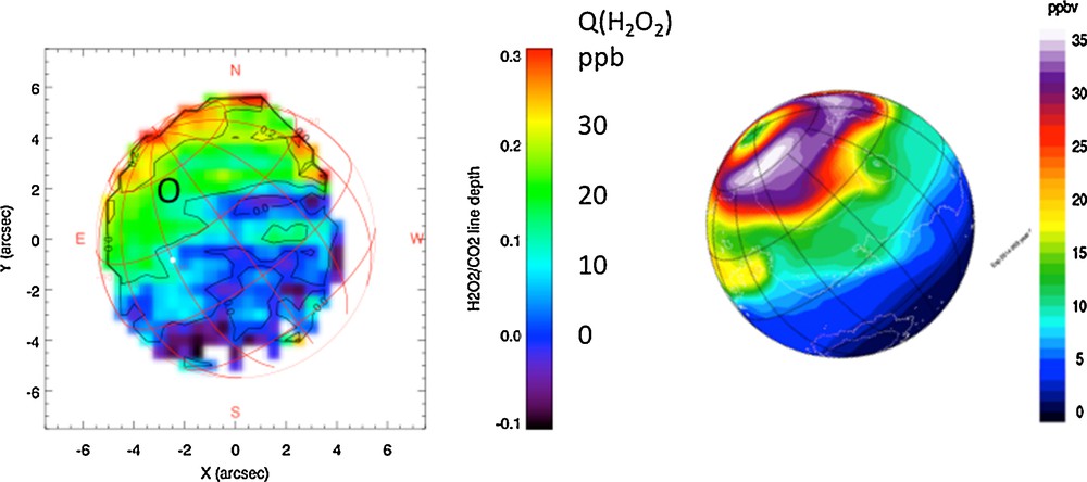
In order to map the H2O2 mixing ratio on the Martian disk, we selected a H2O2 doublet which brackets a weak CO2 line at 1241.6 cm−1, and we simply compute the ratio of the line depths of the H2O2 transitions versus the CO2 transitions. Radiative transfer calculations show that this line depth ratio is a very good indicator of the H2O2/CO2 mixing ratio as it eliminates, to first-order, effects due to geometry and thermal structure. Fig. 1 shows the spectrum of the H2O2 doublet observed in June 2003 (Ls = 206°) at the time of the first detection, and the first H2O2 map recorded for this season.

(Color online.) Top: the TEXES spectrum of Mars (black curve) around 1241.6 cm−1 showing a doublet of H2O2 transitions (at 1241.53 and 1241.61 cm−1) bracketing a CO2 transition (at 1241.58 cm−1). Line positions correspond to rest frequencies. Models: [H2O2] = 20 ppb (green), 40 ppb (red, best fit), and 80 ppb (blue). The spectrum is integrated in a region of the Martian disk where the H2O2 abundance is maximum. Bottom: left: map of the line depth ratio of H2O2/CO2 retrieved from the TEXES data recorded in June, 2003 (Ls = 206°). Right: GCM synthetic map of the H2O2 mixing ratio under the same observing conditions.
The figure is adapted from Encrenaz et al., 2004.
Since 2003, we have been observing H2O2 in November 2005, June 2008, October 2009 March 2014, and July 2014, to monitor its behavior as a function of time and season (Encrenaz et al., 2005, 2008, 2012a,b). As an example, Fig. 2 shows the H2O2 map retrieved with this method in March 2014 (Ls = 96°), compared with the H2O2 map calculated using the LMD-GCM (Forget et al., 1999), including a photochemical model developed at LATMOS (Lefèvre et al., 2008). It can be seen that the H2O2 distribution over the disk is far from being uniform, and globally well fitted by the model. The disk-integrated H2O2 mixing ratio typically ranges between a few ppb and about 30 ppb. The conclusion of these observations is that the H2O2 behavior is well reproduced by the models. In particular, Fig. 3 shows the evolution of the H2O2 content as a function of Ls, compared with various photochemical models. It can be seen that the observations favor the LMD-IPSL model including heterogeneous chemistry on water ice grains (Encrenaz et al., 2012a,b, 2015a; Lefèvre et al., 2008). The same behavior is observed for the seasonal distribution of ozone on Mars, as well as in the terrestrial atmosphere, where the loss of polar ozone in the Earth's stratosphere has been explained by interactions between gaseous chemical species and ice cloud particles (Lefèvre et al., 2008).
(Color online.) Left: map of the line depth ratio of H2O2/CO2 retrieved from the TEXES data recorded on 1 March 2014 (Ls = 96°). Right: GCM synthetic map of the H2O2 mixing ratio under the same observing conditions. Note that the color scales of the two maps are different: the maximum mixing ratio of H2O2 is 35 ppb in both cases.
The figure is adapted from Encrenaz et al. (2015a).
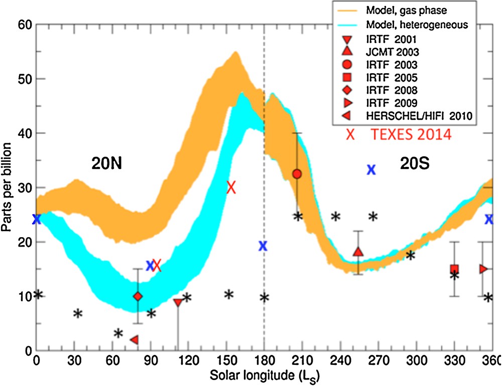
(Color online.) The seasonal cycle of the H2O2 mixing ratio on Mars. TEXES observations refer to 20 N latitudes for Ls = 0–180° and to 20S latitudes for Ls = 180–360°, in order to match as best as possible the observing conditions induced by the axial tip of the planet. Submillimeter observations refer to the entire disk. GCM simulations ignore (yellow) or include (light blue) heterogeneous chemistry. Other 1-D photochemical models are shown for comparison (black stars: Krasnopolsky, 2009; blue crosses: Moudden, 2007). The Herschel point at Ls = 77° corresponds to an upper limit. The two red crosses correspond to the TEXES 2014 observations.
The figure is adapted from Lefèvre et al. (2008).
Using weak HDO transitions in the 1237–1244 cm−1 range, we have simultaneously retrieved maps of water vapor, using HDO as a tracer of H2O. We made the assumption that D/H was constant over the Martian disk, with a value of 5.0 times the terrestrial value (Krasnopolsky et al., 1997). This is actually a first-order approximation, as theoretical calculations predict variations associated, in particular, with condensation (Montmessin et al., 2005). We assume a constant D/H value in the lack of precise measurements. The water vapor seasonal cycle is generally well understood on Mars since the Viking measurements and, more recently, the TES monitoring aboard the MGS orbiter (Smith, 2002, 2004), and maps of the water vapor content versus latitude and areocentric longitude are well represented by GCMs. However, no information has been acquired so far on two-dimensional maps of water vapor that would give, for any season, the H2O distribution versus latitude and longitude, or versus latitude and local hour. This information requires imaging spectroscopic capabilities from some distance, as from the ground or Earth orbit, and has been obtained in the thermal regime for the first time with TEXES. In general, the agreement between the TEXES maps of HDO and H2O maps predicted by the GCM is satisfactory. An example is shown in Fig. 4 for Ls = 80°, just before the northern summer solstice, when water vapor is expected to be maximum. There is a very good agreement between the data and the model (Encrenaz et al., 2010).
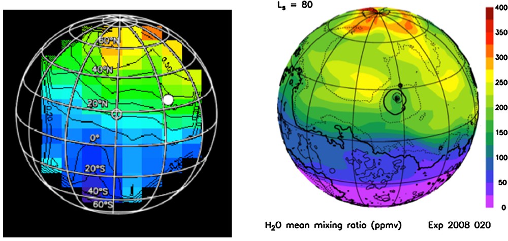
(Color online.) Comparison of TEXES maps and GCM simulations for the June 2008 data set (Ls = 80°). The water vapor mixing ratio is indicated (250 ppm at 30N–50N).
The figure is taken from Encrenaz et al. (2010).
In summary, monitoring the Martian atmosphere using high-resolution ground-based imaging spectroscopy has allowed us to monitor the seasonal variations of hydrogen peroxide and water vapor, and to give indication for H2O2 photochemical models including heterogeneous chemistry. It has also confirmed that the GCM provides a very good understanding of the Martian climate in terms of chemical composition and thermal structure.
3 The atmosphere of Venus
While both Mars and Venus have in common a CO2-dominated atmosphere, with N2, Ar, CO, H2O as minor species, the atmosphere of Venus presents, as compared to the Martian atmosphere, an extreme case with very high surface pressure (90 bar) and temperature (730 K). In addition, sulfur (most likely outgassed from the interior) plays a major role in the photochemistry and dynamics of Venus. The surface of Venus is hidden by an opaque cloud deck, rich in sulfuric acid, extending to altitudes of about 50–65 km.
In contrast with the case of Mars, the atmosphere of Venus is far from being understood in terms of vertical transport and dynamics. Even the mass budget of sulfur is not understood. Indeed, both SO2 and H2O are relatively abundant (150 ppm and 30 ppm respectively) in the lower troposphere, below the cloud deck (Bézard and de Bergh, 2007). Above the clouds, these abundances drop down to about 100 ppb and 1 ppm, respectively (Marcq et al., 2011; Zasova et al., 1993). Assuming that most of water combines with SO2 to form H2SO4, only one fifth of the total SO2 content is used in this process. So in which form is the remaining sulfur? Most likely in the form of aerosols, but their exact nature – and thus their optical and radiative properties – is not known. Above the cloud deck, another surprising result has been found. In the lower mesosphere, the SO2 mixing ratio is known to decrease with altitude, down to a few ppb above the clouds (Belyaev et al., 2012). Then, it increases again in the upper mesosphere, at a level of about 90 km, where SO and SO2 have both been detected in the submillimeter range, at a level of a few tens of ppb (Sandor et al., 2010, 2012). Thus, a second reservoir, probably also made of sulfur aerosols, must be present at these altitudes.
Since 2011, we have been observing water and sulfur species on Venus on different occasions and at different altitudes. In November 2011, we have used the Atacama Large Millimeter Array (ALMA) facility to obtain submillimeter maps of minor species in the upper atmosphere, at an altitude of about 90 km. In January and October 2012, we have used TEXES at IRTF to study the spatio-temporal variations of SO2 and H2O (through its proxy HDO) at the cloud-top and within the clouds. These observations have shown evidence of strong spatial and temporal variations of the sulfur species, both at the cloud-top and in the upper mesosphere. These variations are presently not understood by the photochemical or dynamical models.
3.1 ALMA observations the upper mesosphere
We observed Venus with ALMA in November 2011 during Cycle 0 (Early Science Phase). Alma is an international facility that, using a set of 66 antennas of 7 to 12-m diameter, provides high-resolution heterodyne spectroscopy (R > 106) in spectral atmospheric windows covering the whole millimeter–submillimeter range (80–800 GHz, corresponding to wavelengths of 500 μm–3.7 mm). At the time of our observations, 16 antennas of 12-m diameter were available. Venus was about 11 arcsec in diameter, and we obtained maps with a spatial resolution of about 2 arcsec. We chose a set of transitions near 345 GHz and we observed simultaneously CO at 345.796 GHz, HDO at 335.955 GHz, SO at 346.528 GHz, and SO2 at 346.620 GHz. Four observing runs of 30 min each were recorded on 14, 15, 26 and 27 November 2011, successively. The preliminary results are presented in Encrenaz et al. (2015a).
Fig. 5 shows the variations of SO, SO2 and HDO on 14 and 15 November. The SO map is of best quality because, although SO is less abundant than SO2, the SO transition is intrinsically much stronger. All three species show significant variations over the disk and over a timescale of a day. In the case of HDO, the variations could be associated with fluctuations of the mesospheric temperature; in the case of the sulfur species, the origin of these variations is unknown.
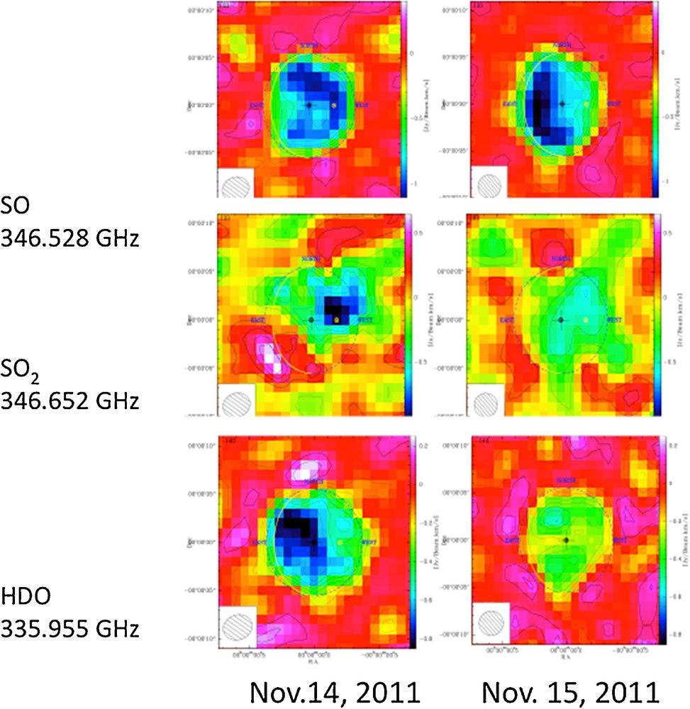
(Color online.) Maps of the intensities of SO (346.528 GHz, top), SO2 (346.652 GHz, middle) and HDO (335.955 GHz, bottom) transitions recorded with ALMA on November 14 (left) and 15 (right), 2011 with the ALMA facility. The submillimeter radiation probes the upper stratosphere (z = 90 km). All species show significant spatial and temporal variations over a timescale of a day.
The figure is adapted from Encrenaz et al. (2015b).
We have also used the disk-integrated spectra of SO, SO2 and HDO on 14 November to infer their mean mixing ratios and vertical distributions. Both sulfur species show a cut-off below the altitude level of 88 km, and mixing ratios of 8 ppb and 12 ppb, respectively, above this level. The HDO vertical distribution, in contrast, is well fitted with a constant H2O mixing ratio of about 2.5 ppm, assuming a D/H ratio of 200 times the terrestrial value in the upper mesosphere (Fedorova et al., 2008).
3.2 TEXES observations of the lower mesosphere
Fig. 6 summarizes the observations of SO2 and HDO obtained in January 2012 over a timescale of 3 days, at the cloud-top of Venus (z = 65 km), using high-resolution spectra around 1350 cm−1 (λ = 7.4 μm). It can be seen that SO2 shows strong spatial variations over the disk, and significant changes within a day; in contrast, the water distribution is much more uniform and constant with time. The maximum mixing ratio of SO2 is about 100 ppb, and the H2O mixing ratio, constant over the disk, is about 1.5 ppm (Encrenaz et al., 2012).

Upper left: maps of HDO recorded at the cloud-top of Venus on January 10 and 12, 2012. The maps show no significant variation over space and time. Upper right: the spectrum of Venus extracted around 1350 cm−1 in a region of maximum SO2 signal, showing transitions of SO2, HDO and CO2. Bottom: maps of SO2 at the cloud-top recorded on January 10, 11 and 12, 2012. Strong variations are observed over the disk and over a timescale of one day.
The figure is adapted from Encrenaz et al. (2012b, 2013).
Subsequent observations of SO2 and HDO, in October 2012, February 2014 and July 2014, have confirmed the high variability of SO2 (over a timescale as short as 2 h) and the more or less constant distribution of H2O over the disk and with time (Encrenaz et al., 2013, 2014a, b, c). In addition, spectra of SO2 have been obtained at 19 μm, where the radiation comes from within the clouds, a few kilometres below the cloud-top. Vertical distributions of SO2 and HDO have been retrieved in areas of maximum abundances. Best fits are obtained with a cut-off in the vertical distribution of SO2 at a level located a few kilometres above the cloud-top. In contrast, the HDO spectra are well fitted with a water vertical distribution constant with altitude. Another interesting result was a drop by a factor 3 of the disk-integrated mixing ratio of SO2 at the cloud-top in February 2014, as compared with the three other runs (Encrenaz et al., 2014b). All these results are globally consistent with Venus Express results taken by SPICAV and SOIR (Belyaev et al., 2012: Marcq et al., 2011), but are presently unexplained by theoretical models.
It is interesting to compare the TEXES and ALMA data, in spite of the time difference (one month) between the two data sets. The SO2 vertical distribution shows a strong depletion a few kilometres above the clouds (z = 67–70 km), then increases again above 90 km. In contrast, the H2O vertical distribution appears to be constant in the mesosphere. The SO2 spatial distribution is patchy and changes over short timescales, both in the lower and upper mesosphere. The H2O distribution is constant with space and time in the lower mesosphere; at higher altitudes where water condensation can take place, the HDO variations might be associated with temperature fluctuations.
4 The future: monitoring the dynamics of Jupiter in support of the Juno mission
In July 2016, the Juno space mission, launched by NASA in August 2011, will encounter Jupiter. One of its main objectives is the measurement of the O/H ratio in the deep interior of the planet, a key measurement for understanding the nature of the planetesimals that formed the planet (Atreya et al., 1999). This measurement will be made in the radio range where water has a major contribution to the continuum spectrum (Janssen et al., 2005). However, other minor species (NH3, PH3, H2S…) also have contributions in this spectral range; in particular, ammonia is a major radio absorber.
Ammonia and phosphine are both tracers of Jovian dynamics. PH3 is a disequilibrium species that is not expected to be observed in the Jovian spectra, as it should react with H2O in the deep troposphere to form P4O6. Its presence in the upper troposphere is due to vertical motions that carry the molecule upward on timescales shorter than the destruction lifetime of the molecule (Lewis, 1997). The presence of NH3, in contrast, is predicted by thermo-chemical models. Its abundance is constrained by reactions with H2O and H2S to form NH4OH and NH4SH clouds at about 2 bar, then by NH3 condensation above the 0.5 bar level (Atreya, 1986). Both ammonia and phosphine are thus tracers of Jovian dynamics; it is important to measure their abundances in the troposphere of Jupiter, and to monitor their possible temporal variations.
In February 2014, we have started an observing program to monitor the abundances of NH3 and PH3 at different atmospheric levels of the Jovian troposphere (with pressure levels ranging from 0.1 bar to a few bars). Using the same technique as that developed for our Mars and Venus observations, we have mapped the Jovian disk in three different spectral ranges probing different pressure levels: 4.64 μm (P = 3–5 bar); 8.83 μm (P = 0.3–0.5 bar); 10.47 μm (P = 0.1–0.3 bar). Preliminary results are given in Fig. 7, which shows maps of the line depths of two specific transitions of NH3 and PH3 at the 0.3–0.5 bar pressure level. It can be seen that both maps are distinctly different, illustrating that both molecules are sensitive to different dynamical mechanisms; in addition, the PH3 abundance seems to be enhanced at high northern latitudes, a trend that is also observed at other pressure levels (Encrenaz et al., 2015b). This work will be pursued in 2015 and beyond, with the objective of mapping the abundances of these two species as a function of time, longitude, and latitude at the time of the Juno mission.

(Color online.) Maps of NH3 and PH3 transitions recorded at 1134.0 cm−1 and 1133.2 cm−1 respectively, probing the 0.5-bar pressure level near the ammonia condensation level. The two maps show significant differences, associated with different transport mechanisms. The PH3 shows a trend for enrichment toward high northern latitudes, also observed at other altitude levels.
The figure is adapted from Encrenaz et al. (2014c).
Acknowledgements
This is an invited contribution to the special issue “Invited contributions of 2014 geoscience laureates of the French Academy of Sciences”. It has been reviewed by Françoise Combes and Editor Vincent Courtillot. The author is most grateful to T. Greathouse, M. Richter and J. Lacy, who have developed and are operating the TEXES instrument, and to A. Tokunaga, Director of IRTF, for the support of the IRTF staff. She is also most grateful to R. Moreno and to the Alma Regional Center in Grenoble for the reduction of the ALMA data. She wants to thank her friends and colleagues from LESIA (B. Bézard, P. Drossart, T. Fouchet, E. Lellouch, R. Moreno, T. Widemann) and from IPSL (F. Forget, F. Lefèvre, F. Montmessin) who have participated in these programs. This work was supported by the Programme national de planétologie, CNRS/INSU.