The reduction of hydrological models for less tedious practical applications

Frederick Delay; Philippe Ackerer

doi:10.1016/j.crte.2015.08.002

Hydrology, Environment (Hydrology–Hydrogeology)

The reduction of hydrological models for less tedious practical applications

Présenté par : Handled by Michel Campillo

Frederick Delay ¹ ; Philippe Ackerer ¹

¹ LHyGeS, université de Strasbourg/EOST – CNRS, 1, rue Blessig, 67000 Strasbourg, France

Comptes Rendus. Géoscience, Volume 348 (2016) no. 2, pp. 89-98.

Résumé

This work evidences that inconsistencies may persist between the complexity of hydrological models and available data for model documentation and application. For example, the integrated hydrological models handle the whole water dynamics over a watershed, but are only conditioned on data that incompletely record the dimensions of the flow. It is suggested to reduce this type of model by aggregating the physical background to diminish its Euclidean dimension. Paradoxically, the complexity in the physics of a model may also result in some reduction. For example, handling a flow by relying upon a dual continuum approach conceals the structural heterogeneity of the reservoir in the model equations. The parameterization at the scale of the aquifer becomes much simpler and the model reduction is here associated with diminishing the effort to condition the model onto data.

Métadonnées

Reçu le : 2015-08-06
Accepté le : 2015-08-28
Publié le : 2015-12-10

DOI : 10.1016/j.crte.2015.08.002

Mots clés : Integrated hydrological model, Flow dimension, Single and dual continua, Inverse problem, Parameterization

Affiliations des auteurs :

Frederick Delay ¹ ; Philippe Ackerer ¹

¹ LHyGeS, université de Strasbourg/EOST – CNRS, 1, rue Blessig, 67000 Strasbourg, France

@article{CRGEOS_2016__348_2_89_0,
     author = {Frederick Delay and Philippe Ackerer},
     title = {The reduction of hydrological models for less tedious practical applications},
     journal = {Comptes Rendus. G\'eoscience},
     pages = {89--98},
     publisher = {Elsevier},
     volume = {348},
     number = {2},
     year = {2016},
     doi = {10.1016/j.crte.2015.08.002},
     language = {en},
}

TY  - JOUR
AU  - Frederick Delay
AU  - Philippe Ackerer
TI  - The reduction of hydrological models for less tedious practical applications
JO  - Comptes Rendus. Géoscience
PY  - 2016
SP  - 89
EP  - 98
VL  - 348
IS  - 2
PB  - Elsevier
DO  - 10.1016/j.crte.2015.08.002
LA  - en
ID  - CRGEOS_2016__348_2_89_0
ER  -

%0 Journal Article
%A Frederick Delay
%A Philippe Ackerer
%T The reduction of hydrological models for less tedious practical applications
%J Comptes Rendus. Géoscience
%D 2016
%P 89-98
%V 348
%N 2
%I Elsevier
%R 10.1016/j.crte.2015.08.002
%G en
%F CRGEOS_2016__348_2_89_0

Frederick Delay; Philippe Ackerer. The reduction of hydrological models for less tedious practical applications. Comptes Rendus. Géoscience, Volume 348 (2016) no. 2, pp. 89-98. doi : 10.1016/j.crte.2015.08.002. https://comptes-rendus.academie-sciences.fr/geoscience/articles/10.1016/j.crte.2015.08.002/

Version originale du texte intégral

1 Introduction

It is duly acknowledged today that subsurface hydrological systems are in essence hard to survey despite the promising results brought by near-surface geophysics imaging (e.g., Hinderer et al., 2009; Mari and Porel, 2008; Mari et al., 2009). Subsurface systems remain usually under-sampled when a key question regarding water resources is to foresee with reasonable confidence how water quality and quantity will evolve under various natural and anthropic stresses.

Very early in the modern history of hydrological sciences, numerical models became alternative solutions filling in the blanks due to lack of data to better understand the dynamics of hydrosystems. Therefore, in the early 1980s, a few numerical spatially distributed models appeared with the aim of simulating groundwater flow. Research efforts rapidly translated into operational tools for practical applications in the public domain (e.g., Ledoux et al., 1989; McDonald and Harbaugh, 1980; Thiery, 1990). These tools were first used as frameworks interpreting the few available data. The raise of various requests from stakeholders and decision-makers in the eighties encouraged the development of modeling tasks aimed at large regional aquifers. A few studies at the local scale came out, but they were built as some kind of specific refinements hosted by the models at the large scale (e.g., Stockle et al., 1994). In any case and until the early 2000s, the focus was put on groundwater flow (and to a less extend on mass transfers); hydro-meteorological fluxes, surface flow and the vadose zone behavior being concealed in very simple inlet-outlet terms of the groundwater system (e.g., Kholghi et al., 1996).

Probably triggered by the research activity on climate changes, works on the continental water cycle rediscovered that surface and subsurface compartments of the cycle were tightly linked together (e.g., Fleckenstein et al., 2010; Winter et al., 1998). The physics of the simple water mass exchanges between surface and subsurface compartments revealed a poor explanation to observation data. In the meantime, the evolutions of stresses on hydrosystems, such as irrigation of the intensive agriculture, have generated new difficulties for the water resources management. One observes that deeper aquifers are rapidly depleted and, in return, severe droughts occur in valleys of large rivers. The accelerated cycling of water also increases groundwater contamination and excess of water mineralization (e.g., Skaggs et al., 1994; Yadav et al., 2002). All the above features were conducive to the development of revisited hydrological models.

The second generation of hydrological models appeared recently. They are also called “integrated” models because they handle three compartments of the water cycle, namely, the surface, the vadose zone, and the subsurface of a watershed (e.g., Frei et al., 2010; Furman, 2008; Goderniaux et al., 2009; VanderKwaak and Loague, 2001; Weill et al., 2013). The hydro-meteorological part in these models is still rough, probably because the identification of meteorological parameters and fluxes at the local scale are yet a fertile research domain with many unanswered questions (local radiative budget, separation between evaporation and vegetation transpiration, etc.; Mirus et al., 2011; Sophocleous, 2002).

While the first generation of groundwater flow models has mostly dealt with large-scale studies and partly homogenized systems (or assumed as such), the integrated models often handle problems at a smaller scale over heterogeneous domains. It must be acknowledged that the dynamics of water fluxes is very contrasted between the surface, the soil, and the aquifer; the characteristic travel time of water being roughly on the order of a few days, a few weeks to a few months, a few months to several years, in the respective compartments. In addition, numerous applications of integrated models target high resolution over small to mid-scale systems (1–1000 km²). The strong structural heterogeneity of the reservoirs (e.g., fractured porous aquifers, soil with multiple porosities…) cannot be overlooked.

The main features evoked above make that the integrated models have become more and more complex and consequently less and less conditioned onto available data. Even if more data are available today, this is mostly because local variables are monitored in time to obtain long histories, regarding for example the flow rates in rivers, the hydraulic head in aquifers, the major dissolved chemical elements. Except for the very specific cases of research experimental sites, some oil fields or underground repositories (e.g., Mari et al., 2009), the “routine” investigations about for instance underground heterogeneity or exchange rates between rivers and aquifers did not evolve very much. Finally, one has at reach, on the one hand, precise three-dimensional and multi-physics models, and on the other hand, very few high-resolution data to document any practical application. In general, complex models are not ensured to escape from the so-called intrinsic equifinality making that the same model outputs may stem from different processes. The consequence is that model predictions become flawed because they rely upon irrelevant settings. The point is not to undermine the technical and scientific advances brought by the integrated models, but their application must pass through a preliminary stage of “reduction” that adjusts the model complexity to conditioning data and expected objectives.

A couple of examples illustrating the notion of model reduction are proposed in the following. Within the framework of calculating surface and subsurface flow and their coupling in small- to mid-size catchment areas, the first example rests on the argument that usual flow data do not distinguish all the flow geometries. For example, flow rate measurements or water levels in rivers provide us with averaged values that do not really see the three-dimensionality of free-surface flow in a draining network. In the same vein, the hydraulic heads in aquifers are often measured as water levels in open boreholes where the hydraulic potential equilibrates at a mean value quite uniform over the wetted thickness of the aquifer. The head sees neither the heterogeneity of the aquifer along the vertical direction nor the vertical component of flow (Delay et al., 2011, 2012). We propose to reduce the surface draining system (ditches, river…) to a connected network of one-dimensional bonds with simplified cross-sections. The subsurface flow is handled over a continuum vadose zone saturated zone via the integration along the vertical direction of both the soil-aquifer hydrodynamic parameters and heads (or capillary pressures). Therefore, the vadose zone and the aquifer are modeled as a single deformed two-dimensional layer (with some thickness), the deformation accounting for the variations in elevation of both the soil surface and the aquifer bottom.

The second example focuses on the aquifer compartment, especially that of fractured porous and/or karstified systems. We mentioned already that the vertical heterogeneity and the vertical fluxes were hardly identifiable on the basis of classical hydraulic head measurements. In the presence of strong heterogeneity, as observed in fractured porous media, a classical approach depicting the geometry of both the fracture network and the porous matrix will be hampered by the lack of information on the fractures. In opposite, a single-continuum approach (a unique porous medium) should be carefully and accurately discretized to show high contrasts of hydrodynamic properties over short distances that allow the occurrences of channeled flows. By keeping a two-dimensional approach to the aquifer but introducing a more complex physics of flow, it becomes possible to reduce the groundwater model. The local heterogeneity of the flow is merged into a dual continuum that depicts explicitly the fluxes in an open network of fractures and the fluxes in the porous matrix. An example at the scale of an experimental site is discussed by solving the inverse problem on the basis of hydraulic interference data between open wells. A single-continuum approach needs highly variable local hydrodynamic properties and a huge model parameterization. Conversely, the more complex physics of flow in a dual continuum depicts the local heterogeneity and only needs a rough spatial resolution on the model's parameters. Incidentally, the model reduction here associated with lighter parameterizations is prone to the so-called “Monte Carlo” uncertainty evaluations of various forecasts by diminishing the calculation efforts for both forward and inverse modeling (e.g., Ginsbourger et al., 2013; Josset et al., 2015).

2 Reduction of dimensionality in an integrated hydrological model

2.1 Flow in the surface draining network

The integrated model is here restricted to flow in the surface draining network and subsurface flow in the vadose and saturated zones. Usually, free-surface flow in draining networks and rivers is handled by means of the Saint-Venant equations (e.g., Panday and Huyakorn, 2004), which will be rewritten hereafter as a one-dimensional equation of diffusive-wave propagation (Govindaraju and Kavvas, 1990). It is assumed that each river segment is of trapezoidal cross section and defined by two main parameters, l [L], the width of the river bottom, and α [–], the slope of the river banks. One also assumes that a mean unit flux (velocity) u_x [LT⁻¹] in the direction x normal to the flow section can be defined. The x direction is not fixed in space and follows the main slope of the riverbed. Under the above conditions, the system of equations associated with the water flux conservation (Eq. (1a)) and the momentum conservation (Eq. (1b)) can be rewritten in the form:

\frac{\partial A}{\partial t} + \nabla_{x} (A u_{x}) = l' q

(1a)

\frac{\partial u_{x}}{\partial t} + u_{x} . \frac{\partial |u_{x}|}{\partial x} + |g| \nabla_{x} h = - |g| (\nabla_{x} z + s_{f}) - \frac{q}{h} u_{x}

(1b)

A [L²] is the surface of water normal to the main flow direction x in the river, h [L] is the water level in the river, l’ [L] is the width of the water surface in the river, z [L] is the elevation, q [LT⁻¹] is the source term of the lateral inlets/outlets along the banks and the bottom of the river,

|g|

[LT⁻²] is the scalar component of the gravity acceleration, s_f [–] is the vector of the so-called “friction” slope of the river.

A major simplification can be applied to the momentum conservation equation by assuming slow variations in the flow regime (a pseudo steady-state flow) that cancel out the term $d / d t = \partial / \partial t + u \partial / \partial x$ . The lateral fluxes q are also assumed negligible compared with fluxes along the main direction of the river bed. Eq. (1b) is rewritten as:

\nabla_{x} (h + z) = - s_{f}

(2)

Even though the velocity u_x has apparently disappeared in Eq. (2), the friction slope s_f reintroduces this velocity by means of the Manning formula:

u_{x} = \frac{R_{h}^{2 / 3}}{N_{man}} s_{f}^{1 / 2}

(3)

with N_man [L^−1/3T] the Manning coefficient, and R_h [L] the hydraulic radius of the river (see below).

For a trapezoidal section of the flow, one easily identifies the width of the water surface l’ and the flow section A as functions of the water level h and the parameters l and α:

l' = l + \frac{2 h}{tan α}; A = \frac{l + l'}{2} h = (l + \frac{h}{tan α}) h

(4)

The hydraulic radius R_h corresponds to the ratio of the section A to the wetted perimeter of the riverbed:

R_{h} = \frac{(l + l') h}{2 (l + 2 h / sin α)}

(5)

Substituting s_f (Eq. (2)) in the Manning formula (Eq. (3)) results in the expression of the mean unit flux along the main flow direction:

u_{x} = - \frac{R_{h}^{2 / 3}}{N_{man} {|\nabla_{x} (h + z)|}^{1 / 2}} \nabla_{x} (h + z)

(6)

Introducing u_x in the flux conservation (Eq. (1a)) yields:

\frac{\partial A}{\partial t} - \nabla_{x} \cdot (A \frac{R_{h}^{2 / 3}}{N_{man} {|\nabla_{x} (h + z)|}^{1 / 2}} \nabla_{x} (h + z)) = l' q

(7)

Noting that the differentiation of A with respect to time can be rewritten as:

\frac{\partial A}{\partial t} = \frac{\partial}{\partial t} (h (l + \frac{h}{tan α})) = (l + \frac{2 h}{tan α}) \frac{\partial h}{\partial t} = l' (h) \frac{\partial h}{\partial t}

(8)

the flux conservation takes the form of a non-linear one-dimensional diffusion equation for the water level h in the river.

l' (h) \frac{\partial h}{\partial t} - \nabla_{x} (T_{R} (h) \nabla_{x} (h + z)) = l' (h) q; T_{R} (h) = \frac{(l + l' (h)) h R_{h}^{2 / 3}}{2 N_{man} {|\nabla_{x} (h + z)|}^{1 / 2}}

(9)

2.2 Flow in the vadose and saturated zones

The subsurface compartment bounded between the soil surface and the bottom of the aquifer is handled as a single continuum. For the sake of simplification, we overlook the eventual existence of gravitational flow in the form of thin water layers at the topographic surface (Hortonian flow) and of shallow underground water layers favored by weakly permeable soil horizons (hypodermic flow). These features could also be handled in the same way as for the draining network, but this time relying upon two-dimensional diffusion-wave propagation. Fluxes in the vadose and saturated zones are ruled by Darcian flow and the mass conservation principle. Assuming a weakly deformable porous medium and a constant fluid mass density (i.e. negligible fluid compressibility and absence of large variations in solute content), the equation of flow becomes (e.g., Huyakorn and Pinder, 1983):

\frac{\partial θ}{\partial t} + S s S w (θ) \frac{\partial h}{\partial t} - \nabla \cdot (K (θ) \nabla h) = q_{w}

(10)

θ [–] is the volumetric water content, i.e., the ratio of the water volume to the bulk volume of the medium (pores + solid), Sw [–] is the water saturation, i.e., the ratio of the water volume to the pore volume, Ss [L⁻¹] is the specific storage capacity of the medium, K [LT⁻¹] is the hydraulic conductivity of the medium, h [L] is the hydraulic head (or the capillary head), and q_w [T⁻¹] is a source term (in inlet/outlet water volume per unit volume of medium and unit of time).

The reduction in the flow dimension is performed by the integration of Eq. (10) along the vertical direction z or, in the case of sloping watersheds, along z taken as the direction normal to the aquifer bottom. This procedure may appear awkward, especially in the vadose zone, where for instance infiltration mostly occurs along the vertical direction. The integration of the flow equation will hide the vertical components of flow but not the saturation–desaturation of the system. Because vertical transfers in the vadose zone develop over a few meters when lateral transfers in a watershed occur over several hundred meters, the simplification holds at the scale of the whole hydrological system.

To simplify the integration (namely, to avoid the complete development of a Leibnitz integration), we state that the flow is mainly parallel to the aquifer bottom $(\nabla_{z} h = 0)$ , and that the integration bounds $z_{b}, z_{s}$ corresponding to the elevations of the aquifer bottom and the soil surface, respectively, are of negligible gradients. Finally, the integration along the z direction is split in two components by introducing the integration bound z_w that is the elevation of the saturated–non-saturated interface (or the top of a semi-confined aquifer). The integration of Eq. (10) yields:

\begin{array}{l} \frac{\partial h}{\partial t} \int_{z_{b}}^{z_{w}} S s \cdot S w (θ) d z + \int_{z_{b}}^{z_{w}} \frac{\partial θ}{\partial t} d z + \frac{\partial h}{\partial t} \int_{z_{w}}^{z_{s}} S s \cdot S w (θ) d z + \int_{z_{w}}^{z_{s}} \frac{\partial θ}{\partial t} d z \\ - \nabla_{x, y} \cdot (\nabla_{x, y} h \int_{z_{b}}^{z_{w}} K (θ) d z + \nabla_{x, y} h \int_{z_{w}}^{z_{s}} K (θ) d z) = Q \end{array}

(11)

The splitting allows separating the different behaviors of the hydrodynamic parameters between the vadose and saturated zones. It is obvious that the water content θ does not vary in time in the saturated zone and the water saturation Sw is one. The term in Eq. (11) including the specific storage capacity is negligible compared with the variations of water content in the vadose zone, and finally, the hydraulic conductivity does not depend on the water content in the saturated zone. With these simplifications, Eq. (11) can be rewritten as:

\frac{\partial h}{\partial t} \int_{z_{b}}^{z_{w}} S s d z + \int_{z_{w}}^{z_{s}} \frac{\partial θ}{\partial t} d z - \nabla_{x, y} \cdot (\nabla_{x, y} h \int_{z_{b}}^{z_{w}} K d z + \nabla_{x, y} h \int_{z_{w}}^{z_{s}} K (θ) d z) = Q

(12)

The mean value theorem allows us to express the integrals concealing Ss and K in the form $\int S s d z = S_{Sat} h, \int K d z = K_{Sat} h$ . The term in θ is transformed by introducing the capillary capacity C (h) corresponding to the derivative of the water content with respect to the capillary pressure (or head):

\int_{z_{w}}^{z_{s}} \frac{\partial θ}{\partial t} d z = \int_{z_{w}}^{z_{s}} \frac{\partial θ}{\partial h} \frac{\partial h}{\partial t} d z = \frac{\partial h}{\partial t} \int_{z_{w}}^{z_{s}} C (h) d z

(13)

Finally, the integration along the z direction yields a single two-dimensional flow equation common to both the vadose and saturated zone in the form:

\begin{array}{l} \bar{S} (h) \frac{\partial h}{\partial t} - \nabla_{x, y} \cdot (\bar{T} (h) \nabla_{x, y} h) = Q \\ \bar{S} (h) = S_{Sat} h + \int_{z_{w}}^{z_{s}} C (h) d z; \bar{T} (h) = K_{Sat} h + \int_{z_{w}}^{z_{s}} K (θ) d z \end{array}

(14)

The mean parameters $\bar{S} and \bar{T}$ are calculated by numerical integration. In the vadose zone, this calculation between z_w and z_s assumes that we prescribe the state equations linking the conductivity K with the water content θ and the capillary capacity C with the head h. In addition, these state equations assume that the capillary pressure profile along z is known, when Eq. (14) merely calculates a single mean head value along z. To overcome the problem and to be consistent with the depth-averaged calculation, it is stated that the calculation of $\bar{S} and \bar{T}$ is based on a hydrostatic profile in the vadose zone yielding a linear evolution of the capillary head between zero in z_w and $- (z_{s} - z_{w})$ in z_s. Notably, by assuming a hydrostatic profile that equilibrates instantaneously with the variations of saturated heads (the capillary profile starts at zero in z_w, i.e., the head in the saturated zone), the vertical component of flow in the vadose zone “naturally” cancels out. But as stated earlier, it does not mean that the vadose zone in not sensitive to infiltration and other sink-source terms.

It must also be noted that the flow equation (Eq. (14)) calculates a positive mean head value h whenever the medium is locally saturated (presence of a water table). A negative h value can only be obtained when the whole profile along z is unsaturated (absence of water table). Usually, the lateral fluxes (in the plane normal to z) are such that the hydraulic head gradients and the capillary pressure (h negative) gradient trigger water motion in the saturated zone and the vadose zone, respectively. With only a single value of h per location (x, y), the total lateral fluxes are partly flawed; for example the fluxes in the vadose zone can be the consequence of the head gradient (h positive) in the aquifer. Several tests over various configurations of the medium heterogeneity have been performed. They show that the errors stemming from the integration over the z direction of the flow parameters and head values stay small and non-significant at the scale of the whole watershed. For example, comparing a three-dimensional approach to the flow and the reduced model over hilly catchment areas (see the example of the Strengbach watershed, below) yields errors of 3–5% on heads and water fluxes in the subsurface compartment. Errors in arrival times of, e.g., a rainfall event into a draining network barely exceed 5–10%.

To complete the model reduction, the coupling between the surface drainage network and the subsurface system is carried out by exchanging local fluxes between compartments. These fluxes are assigned via the source terms $l' (h) q$ in Eq. (9) and Q in Eq. (14). They are stated as being proportional to the difference between the water level in the river and the hydraulic head in the aquifer (Gunduz and Aral, 2005). This assumption is reasonable whenever the head in the aquifer is above the elevation of the river bottom. When the water table is lower, the exchange flux simply becomes proportional to the water thickness in the river.

The model reduction in its Euclidean dimension obviously diminishes the computation costs and also simplifies the linearization of the equations in the vadose zone and the draining network. One may reasonably foresee that the calculation costs are at least decreased proportionally to the number of unknowns eliminated by the dimension reduction. For example, a three-dimensional model with 10 “layers” (a minimum for a 3D view on the flow problem) will be calculated at least ten times quicker in its two-dimensional approach (depending on the solver used).

2.3 Example

For the sake of concision, we will not discuss here the comparison between different modeling approaches. We only focus on the model with reduced dimensionality depicted above to show that it behaves correctly, even when handling complex watershed geometry and very transient flow. The example is built on a realistic geometry that borrows the main characteristics of a small water catchment in a hilly region (Le Strengbach, Vosges Mountains, France). The initial geometry is slightly modified in the present exercise to build a reactive system amplifying the responses for easier interpretations. The surface draining network is made of 72 segments, 1 m in width, 1 m in depth, and with vertical banks. The small catchment (0.8 km²) is of stiff slope (about 20–30%), passing in less than 1 km from 1148 m at the highest elevation down to 883 m at the lowest elevation (Fig. 1). This characteristic favors flows mainly controlled by gravity, even in the shallow aquifer of 8 m in thickness over the whole domain. Because of the stiff slopes, the two-dimensional meshing of the subsurface compartment is refined close to the draining network to improve the calculation of surface–subsurface exchanges. Nevertheless, the minimal mesh size never drops below 5 m (Fig. 1).

Fig. 1
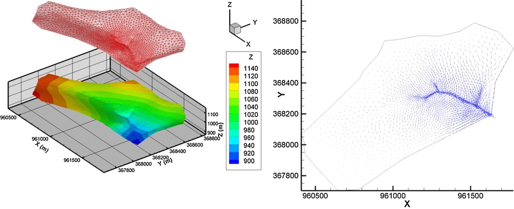
Left, topography and meshing of a small hilly watershed. Right, map of the unit fluxes after 12 h of draining.

The rapid draining from high to low elevations is simulated over 120 h knowing that the initial water table varies linearly between depths of –8 and –4 m below the topographic surface from the highest to the lowest elevations. It is only reported on the evolution of the subsurface compartment. The progressive draining is accurately depicted in space and time. The high elevation areas dry when the valleys collect water, especially those with a river in their bottom, the highly permeable drain making fluid transfers much easier. Overall, for all the simulation times, the fluxes converge toward the surface draining network (Fig. 1) and the size of drained areas shrinks with time since the aquifer dewaters. The maps of hydraulic heads (Fig. 2) confirm the rapid evolution in time of the catchment with a gravity driven flow because of the stiff slopes.

Fig. 2
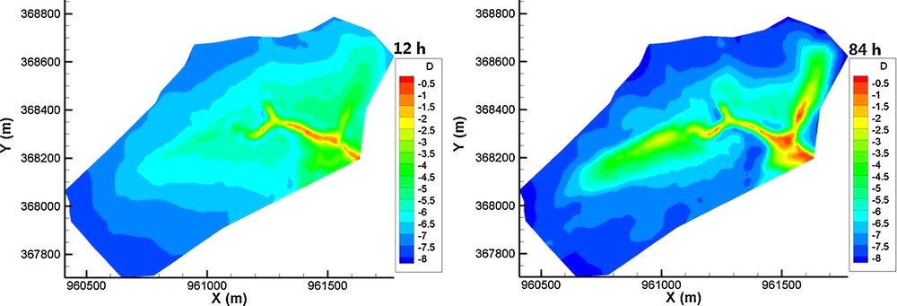
Maps of hydraulic heads during the draining of a small hilly watershed. The heads are expressed as the depth of the water-saturated interface below the topographic surface.

As told above, when discussing the technique reducing the dimensionality of the model, errors at the scale of transfers over the whole watershed are small compared with a fully dimensioned (3D) approach. However, it must be mentioned that the simulation exercise does not include contrasted heterogeneities within the subsurface compartment. This characteristic is purposely set up because one deals with a thin companion aquifer of a small river network. Accounting for significant heterogeneity in the subsurface flow can be done at a larger scale. Regarding the structural heterogeneity of deeper aquifers, the proposal of model reduction by means of an enhanced physics of flow reveals well suited.

3 Model reduction for highly heterogeneous subsurface flow

As already mentioned in the introduction, underground reservoirs may conceal structural heterogeneities hardly visible on hydraulic data. This is the case of limestone aquifers mixing hydrodynamic characteristics of both porous and fractured media over very short distances. The diffusive behavior of Darcian flow smooths out the hydraulic head spatial distribution, making that passing from spread flow in the matrix to channeled flow in fractures is not evidenced by significant head variations (e.g., Kaczmaryk and Delay, 2007a). It becomes very difficult to identify hydraulic property contrasts on the basis of hydraulic head measurements. The flow model must be highly refined and parameterized, which results in cumbersome manipulations for various tasks such as inversion, prediction, and uncertainty evaluation.

Most operational subsurface models deal with complex systems by resorting to a single continuum that is finely spatially discretized and associated with mesh-to-mesh contrasted properties to simulate the structural heterogeneity. The flow is simulated by a single equation merging Darcian fluxes into a mass balance principle. Dropping the initial and boundary conditions, and overlooking references to time and space for lighter writing, the flow model is based on the following equation (e.g., De Marsily, 1996):

S s \frac{\partial h}{\partial t} - \nabla \cdot (K \cdot \nabla h) = q

(15)

h [L] is the hydraulic head in the aquifer, K [LT⁻¹] is the hydraulic conductivity, Ss [L⁻¹] is the specific storage capacity, and q [T⁻¹] a source term per unit volume of the medium. Disparity in space (and eventually in time) of the parameter values Ss and K depicts the structural heterogeneity.

One can also translate the hydrodynamic contrasts in a porous and fractured medium by stating that, in each location, it exists a fracture continuum, highly conductive but weakly capacitive, and a matrix continuum, weakly conductive but highly capacitive (e.g., Barrenblatt et al., 1960; Delay et al., 2007; Warren and Root, 1963). Flow is then ruled by two equations:

\begin{array}{l} S s_{f} \frac{\partial h_{f}}{\partial t} - \nabla \cdot (K_{f} \cdot \nabla h_{f}) + α (h_{f} - h_{m}) = q_{f} \\ S s_{m} \frac{\partial h_{m}}{\partial t} - \nabla \cdot (K_{m} \cdot \nabla h_{m}) + α (h_{m} - h_{f}) = q_{m} \end{array}

(16)

The definitions of h, Ss, K, and q are similar to that formulated in Eq. (15), knowing that specifically, the indexes f and m refer to fracture and matrix continua, respectively. α [L⁻¹T⁻¹] is the flux exchange rate between continua. Several model configurations are possible. Assuming that both media are present everywhere, the Eqs. (16) are documented regarding their parameters in each mesh discretizing the domain. One may also assert that only one medium can exist at a given location and therefore, the parameters of the other medium and the exchange α are set to zero. Nevertheless, this configuration has few interest because the model becomes similar to a single-continuum approach (Eq. (15)), eventually showing a bimodal distribution of the parameters. Finally, it is also frequently assumed (as we do in the following example) that the matrix has a negligible hydraulic conductivity K_m compared to that of the fractures (Landereau et al., 2001). The matrix continuum becomes stagnant, similar to a static reservoir feeding (fed by) the fracture medium via first-order kinetics:

S s_{m} \frac{\partial h_{m}}{\partial t} + α (h_{m} - h_{f}) - q_{m} = 0

(17)

Operational flow models usually do no rely upon a dual continuum because: (1) the parameterization per mesh is larger, with five parameters (excluding the source term) instead of 2 for a single continuum; (2) the very similar form of both flow equations results in equifinalities on the model outputs, except in the case of very contrasted properties between the fracture and matrix continua. It is also true that the heads h_f and h_m are of very different sensitivity with respect to parameters (several orders of magnitude). For example, it is almost impossible to fit the rate α if the other parameters are not prescribed or their sensitivity strongly reduced (Delay et al., 2007; Kaczmaryk and Delay, 2007b). Nevertheless, the example below shows that the dual continuum approach has some advantages regarding model reduction, especially within the exercise of model parameterization and inversion.

The example discussed here is grounded in the inversion of both a single and a dual continuum with reference data drawn from hydraulic interference testing performed at the Hydrogeological Experimental Site (HES) in Poitiers (France). The general depiction of the site and details on interference data can be found in several references, in particular Kaczmaryk and Delay (2007b), Audouin et al. (2008), and Bodin et al. (2012). Interference testing consists in pumping at a constant flow rate in a given well and monitoring the evolution in time of the hydraulic head drawdowns in one or several other distant wells. As stated in the introduction, the mean hydraulic heads measured in open boreholes over the whole thickness of the aquifer poorly record the vertical components of the flow. Therefore, the two models (single and dual continua) assume that the flow is mostly planar horizontal, yielding a two-dimensional discretization of the model equations. The dual continuum also assumes that (1) the matrix is a static reservoir in which the head-gradient-triggered flow is negligible (the hydraulic conductivity K_m is set to zero, see above), (2) heads observed in open boreholes over the whole thickness of the aquifer equilibrate to the mean heads in the fracture continuum. In the specific case of the HES, the limestone aquifer is karstified along four horizontal layers of 2–4 m in thickness at depths 30, 50, 80, and 110 m, approximately. Preferential flow in these layers generates very rapid responses to interference testing.

To better inform the models, one generates interference data sets that add sequentially in time the response of the observed well to each stress generated by each pumped well. The response in each observed well corresponds then to head drawdowns generated by n wells pumped in sequence. Each pumping stress period is followed by a relaxation period allowing the water table to come back to its initial level before pumping (Fig. 3). The data sets at each observed well are used to identify the hydrodynamic parameters of the flow models. One calculates an objective function F(h(p),h*,p) as the sum of the squared errors between the model outputs h(p) and the observations h*. The parameters p are fitted with an optimization algorithm that seeks the best values of p to minimize F. This optimization needs for the calculations of the gradient components $d F / d p$ of the objective function. These components are calculated relying upon an adjoint state method that an interested reader can find in Ackerer and Delay (2010) and Ackerer et al. (2014).

Fig. 3
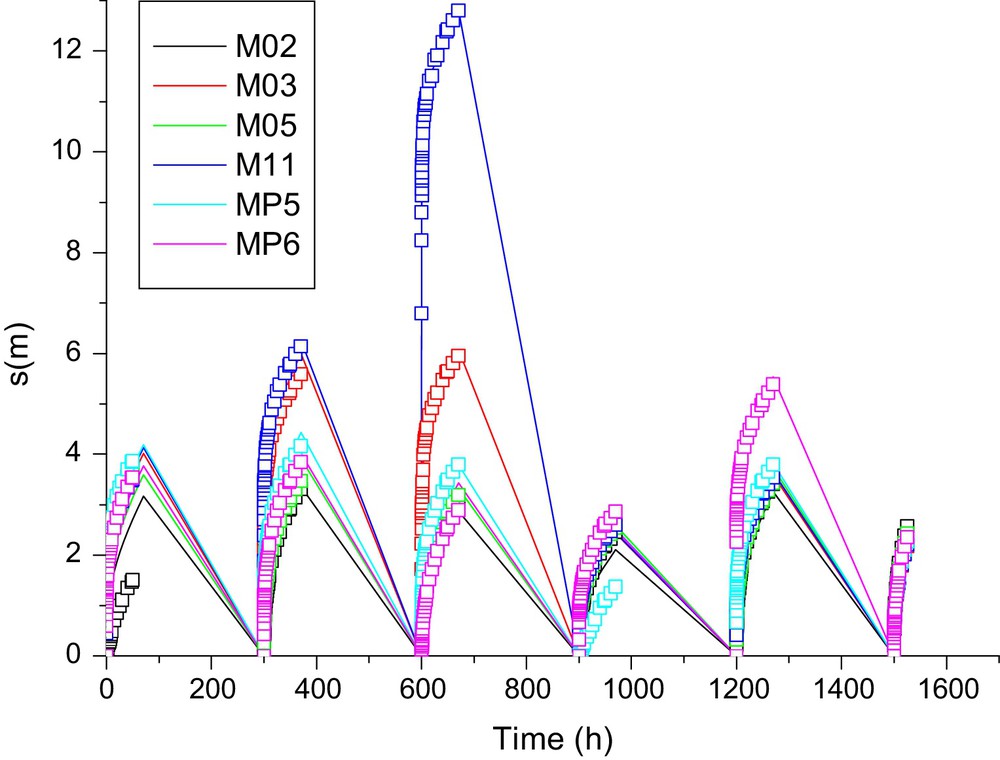
Example of drawdowns from interference testing held in the Hydrogeological Experimental Site (HES) in Poitiers, France. The multiple-peak curves stem from adding sequentially in time the responses in a well to stresses generated by several pumping wells. Dots = observation data, solid lines = outputs of a dual continuum model after inversion.

Provided that both models are coded with the same numerical technique and the same level of space and time discretization, the model reduction is here in the parameterization. One seeks the number and the value of spatially distributed parameters to depict the medium heterogeneity identifiable on interference data. To avoid any influence of the user on the number, the spatial and the statistical distributions of parameters, a specific evolutionary parameterization technique is used (Ackerer and Delay, 2010; Ackerer et al., 2014; Trottier et al., 2014). Local parameter values are set at the nodes of a coarse grid superimposed to the calculation domain. There is no relationship between the parameter grid and the computation grid of the flow equations. Assigning local parameter values to the computation grid is performed by simply interpolating linearly the node values of the parameter grid. Within the convergence iterations minimizing the objective function F, the parameter grid can be refined, thus increasing the number of sought parameters to fit the model (Fig. 4). This refining is local, increasing the number of parameters over areas that show too large local errors $h (p, x, y, t) - h^{*} (x, y, t)$ and/or too large components $d F / d p (x, y)$ . Finally, the successive steps of parameter grid refinements result in a set of local parameter values (at the nodes of the parameter grid) serving as seeds to interpolate the whole parameter field used in the forward model. Because there is no prior guess either on the structure of this parameter field or on the number of seeds requested to calculate it, the parameterization technique provides us with the minimal number of seeds for getting parameter fields that allow model outputs to fit the data. This number is therefore only conditioned by available data, by the physics of the model, and, to a lesser extent, by the interpolation technique between the parameter grid and the computation grid. In the example discussed here, all types of parameters (e.g., K and S_s) have been inverted, each type having its own parameter grid, a priori independent of that of the others.

Fig. 4
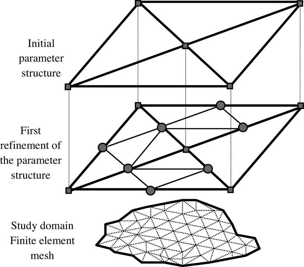
Parameter grid and its refinement steps used in the parameterization of flow models. Prescribing parameter values to the calculation grid (below) rests on a linear interpolation of the seed values at the nodes of the parameter grid.

Regarding the hydraulic interferences mentioned above, Fig. 5 shows as an example of two maps of hydraulic conductivity K (single continuum), K_f (dual continuum) obtained on the computation grid after inversion (Ackerer and Delay, 2010; Trottier et al., 2014). With the flow in the matrix of a dual continuum being negligible, it is reminded that the fracture hydraulic conductivity K_f becomes comparable to the conductivity K of a single continuum. While model fittings on data are of the same quality (usually, less than a one-centimeter error for each head between models and data), the spatial distributions of K and K_f are completely different. At the scale of the whole modeled domain, both approaches identify quite similar variation ranges of parameters. Local conductivity values are usually log normally distributed. The spatial delineation of high versus low conductivity sub-areas may vary between models. However, the parameterization technique depicted above is stochastic in essence and can duplicate the number of equiprobable parameter fields sought by inversion. The ensemble of solutions are relatively narrow and show that on average, the single and dual continua identify similar areas of low and high conductivity. The main difference between the approaches is in the refinement degree required to obtain a model fitting accurately the data. The single continuum has to discretize finely the local heterogeneity to account for results from interference testing. The hydraulic conductivity map may show high contrasts of values between neighbor locations to mimic the contrasted hydraulic behavior of the aquifer. In practice, a large number of local parameters serving as seeds for the interpolation are required to produce the conductivity field. In opposite, the dual continuum encloses in its equations the capability to account for local contrasts in hydraulic behavior. The conductivity map looks like a simple patchwork putting side-by-side large areas of quite uniform values. The map is built with few seed points, i.e., few parameters to identify. For the example above, a single continuum with two types of parameters K and Ss requires between 2 × 1036 = 2072 and 2 × 4108 = 8216 parameters for a valuable inversion. The dual continuum is far less greedy and an inverse solution for the four types of parameters K_f, Ss_f, α, and Ss_m, is found with 4 × 41 = 124 to 4 × 89 = 356 parameter values.

Fig. 5
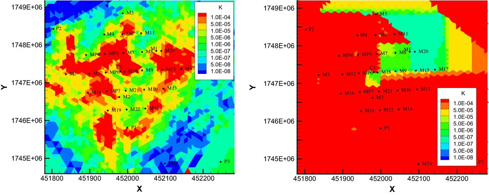
Examples of hydraulic conductivity fields K (single continuum, left), K_f (dual continuum, right) sought by inversion handling of hydraulic interference data. The single continuum needs much more details in the spatial resolution of the conductivity field to provide a valuable inverse solution.

When the numerical resolution of the flow equations is well coded, the calculation cost of a simulation with the dual continuum is barely heavier than that of a single continuum. Although the refinement procedure on the parameter grid party depends on the “randomization” seeking several equiprobable solutions, one may roughly consider that the total computation time is proportional to the number of parameters to identify. In the present case, a dual continuum approach reveals 6 to 66 times quicker to invert than a single-continuum approach. In the end, the enhanced physics of flow results in a drastic model reduction in terms of parameterization and inversion. Regarding the capabilities to provide better forecasts with a reduced model, the answer is not straightforward. Faster computations allow an easier duplication of simulations and perhaps a better assessment of bounds on parameter uncertainty and model outputs. However, in the present case both models return very similar joint-parameter distributions. Therefore, in a Bayesian context, the credibility of model forecasts is mainly associated with the sensitivity of the model to parameters, or stated differently, with the likelihood of model outputs knowing the parameters. Along this line, and provided that models with different physics are comparable, both single and dual continua have similar sensitivities to conductivity and storage capacity.

4 Conclusion

It is acknowledged that detailed investigations on the water cycle are relevant topics for many research works and practical applications. This activity generates more complex physically-based hydrological models. For instance, the so-called “integrated” models enclose in the same framework the complexity of a watershed from hydro-meteorological inlets, surface drainage, and infiltration in soils, to subsurface flow. This being said, a model is still a generic tool that must be documented to become applicable.

The chronic undersampling of hydrosystems, especially the subsurface compartment, does not help to the model documentation, knowing that the need for data is all the more urgent that the model is complex and of high resolution. Even worse, most of the observed variables weakly discriminate the subtle mechanisms occurring in the hydrosystem. We took the example of the flow rates and water levels in rivers that do not see the three-dimensionality of flow.

These considerations led us to degrade a hydrological model, while avoiding ruining the enclosed physics. The latter is preserved because it is simply “aggregated” to diminish the flow dimensions in the hydrological system. There is no conception error between the dimension reduction, the variables, and the model parameters. Specifically regarding the parameters, the obtained mean values are the strict consequence of the aggregation and not empirical estimates or algebraic manipulations without relationship with the way the model is reduced. Since the idea of model reduction is motivated by the fact of rendering the model variables compatible with observation data, one avoids facing the model outputs with irrelevant data. This feature may become a key point to success in the exercise of model inversion.

Even though multiplying the mechanisms in a model may increase complexity, a sharper physics may also help to model reduction. A simple approach will lump on its own mechanisms the effects of the missing mechanisms that are absent, but partly witnessed by data. Therefore, a model–data comparison may reveal flawed and generate cumbersome model parameterization with unrealistic parameter values. By taking the example of channeled flows in a karstified limestone aquifer, we show that the model parameterization is strongly reduced by relying upon a physics including the local dichotomy between flow in a fracture continuum and a matrix continuum. Inversion exercises become affordable, especially within a stochastic framework duplicating the search of equiprobable parameter fields.

In general, model reduction also goes with lighter parameterizations. This association may reveal useful when assessing the credibility of model forecasts. Lighter forward and inverse modeling tasks favor the classical procedure of duplicating scenarios to foresee how systems could behave when faced with uncertain constraints. However, it does not mean that a reduced model will result in better (less uncertain) forecasts. For example, if after inversion complex and reduced models render similar values of parameter probability density functions, the forecasts become mainly dependent on the sensitivity of the model to the parameters. It is not sure at all that a reduced model is less sensitive to parameters than a complex model. Nevertheless, a reduced model that adapts its outputs to available data lowers “artificial” errors between data and model outputs, with the well-known incidence of reducing uncertainty in the sought parameters sets of inversion exercises. Also, in the presence of limited available data, the lighter parameterization of reduced models is prone to provide better scores with respect to model selection criteria that compare the parameterization effort to the mass of data conditioning the model.

With no doubt, numerical models have to progress by following the advances on the understanding of how natural systems behave. One ought to also question the compatibility between the model's complexity and the capability to document it, especially in the comparison model outputs–observation data. An idealized view that would build any experimentation or collect information with the full knowledge of the model capabilities and requirements is in practice never fulfilled. Therefore, seeking tangible progress in model developments is probably a problem with two entrances: on the one hand, increasing the complexity to ameliorate the system depiction, on the other hand reducing in full knowledge, the complexity according to the needs and/or available data.

Bibliographie

[Ackerer and Delay, 2010] P. Ackerer; F. Delay Inversion of a set of well-test interferences in a fractured limestone aquifer by using an automatic downscaling parameterization technique, J. Hydrol., Volume 389 (2010), pp. 42-56

[Ackerer et al., 2014] P. Ackerer; N. Trottier; F. Delay Flow in double porosity aquifers: parameter estimation using an adaptive multiscale approach, Adv. Water Resour., Volume 73 (2014), pp. 108-122

[Audouin et al., 2008] O. Audouin; J. Bodin; G. Porel; B. Bourbiaux Flowpath structure in a limestone aquifer: multi-borehole logging investigations at the Hydrogeological Experimental Site of Poitiers – France, Hydrogeol. J., Volume 16 (2008) no. 5, pp. 939-950

[Barrenblatt et al., 1960] G. Barrenblatt; I. Zheltov; I. Kochina Basic concepts in the theory of seepage of homogeneous liquids in fissured rocks, J. Appl. Math. Mech., Volume 24 (1960), pp. 852-864

[Bodin et al., 2012] J. Bodin; P. Ackerer; A. Boisson; B. Bourbiaux; D. Bruel; J.-R. de Dreuzy; F. Delay; G. Porel; A. Pourpak Predictive modeling of hydraulic head responses to dipole flow experiments in a fractured/karstified limestone aquifer: insights from a comparison of five modeling approaches to real-field experiments, J. Hydrol., Volume 454–455 (2012), pp. 82-100

[Delay et al., 2012] F. Delay; P. Ackerer; B. Belfort; A. Guadagnini On the emergence of reciprocity gaps during interference pumping tests in unconfined aquifers, Adv. Water Resour., Volume 46 (2012), pp. 11-19

[Delay et al., 2011] F. Delay; P. Ackerer; A. Guadagnini Theoretical analysis and field evidence of reciprocity gaps during interference pumping tests, Adv. Water Resour., Volume 34 (2011), pp. 592-606

[Delay et al., 2007] F. Delay; A. Kaczmaryk; P. Ackerer Inversion of interference hydraulic pumping tests in both homogeneous and fractal dual media, Adv. Water Resour., Volume 30 (2007) no. 3, pp. 314-334

[De Marsily, 1996] G. De Marsily Quantitative hydrogeology: groundwater hydrology for engineers, Academic Press, San Diego, CA, 1996

[Fleckenstein et al., 2010] J.H. Fleckenstein; S. Krause; D.M. Hannah; F. Boano Groundwater–surface water interactions: new methods and models to improve understanding of processes and dynamics, Adv. Water Resour., Volume 33 (2010) no. 11, pp. 1291-1295

[Frei et al., 2010] S. Frei; G. Lischeid; J.H. Fleckenstein Effects of microtopography on surface-subsurface exchange and runoff generation in a virtual riparian wetland: a modeling study, Adv. Water Resour., Volume 33 (2010) no. 11, pp. 1388-1401

[Furman, 2008] A. Furman Modeling coupled surface-subsurface flow processes: a review, Vadose Zone J., Volume 7 (2008) no. 2, pp. 741-756

[Ginsbourger et al., 2013] D. Ginsbourger; B. Rosspopoff; G. Pirot; N. Durrande; P. Renard Distance-based kriging relying on proxy simulations for inverse conditioning, Adv. Water Resour., Volume 52 (2013) no. 2, pp. 275-291

[Goderniaux et al., 2009] P. Goderniaux; S. Brouyere; H.J. Fowler; S. Blekinsop; R. Therrien; P. Orban; A. Dassargues Large scale surface-subsurface hydrological model to assess climate change impacts on groundwater reserves, J. Hydrol., Volume 373 (2009), pp. 122-138

[Govindaraju and Kavvas, 1990] R. Govindaraju; M. Kavvas Approximate analytical solutions for overland flow, Water Resour. Res., Volume 26 (1990) no. 12, pp. 2903-2912

[Gunduz and Aral, 2005] O. Gunduz; M.M. Aral River networks and groundwater flow: a simultaneous solution of a coupled system, J. Hydrol., Volume 301 (2005) no. 1–4, pp. 216-234

[Hinderer et al., 2009] J. Hinderer; C. De linage; J.-P. Boy; P. Gegout; F. Masson The GHYRAF (Gravity and Hydrology in Africa) experiment: description and first results, J. Geodyn., Volume 48 (2009) no. 3–5.

[Huyakorn and Pinder, 1983] P.S. Huyakorn; G.F. Pinder Computational methods in subsurface flow, Academic Press, Orlando, FL, 1983

[Josset et al., 2015] L. Josset; D. Ginsbourger; I. Lunati Functional error modeling for uncertainty quantification in hydrogeology, Water Resour. Res., Volume 51 (2015) no. 2, pp. 1050-1069 | DOI

[Kaczmaryk and Delay, 2007a] A. Kaczmaryk; F. Delay Improving dual-porosity-medium approaches to account for karstic flow in a fractured limestone. Application to the automatic inversion of hydraulic interference tests, J. Hydrol., Volume 347 (2007), pp. 391-403

[Kaczmaryk and Delay, 2007b] A. Kaczmaryk; F. Delay Interpretation of interference pumping test in fractured limestone by means of dual-medium approaches, J. Hydrol., Volume 337 (2007), pp. 133-146

[Kholghi et al., 1996] M. Kholghi; M. Razack; W. Treichel Modeling and quantitative management of river-aquifer systems with the use of unit response functions, Hydrogeol. J., Volume 4 (1996), pp. 11-20

[Landereau et al., 2001] P. Landereau; B. Noetinger; M. Quintard Quasi-steady two equation models for diffusive transport in fractured porous media: large-scale properties for densely fractured systems, Adv. Water Resour., Volume 24 (2001) no. 6, pp. 863-876

[Ledoux et al., 1989] E. Ledoux; G. Girard; G. de Marsily; J.-P. Villeneuve; J. Deschene Spatially distributed modeling: conceptual approach coupling surface water and groundwater (H.J. Morel-Seytoux, ed.), “Flow in Hydrologic Modeling”, 275, NATO ASI Series, 1989, pp. 435-454

[Mari and Porel, 2008] J.-L. Mari; G. Porel 3-D seismic imaging of a near-surface heterogeneous aquifer: a case study, Oil Gas Sci. Technol., Volume 63 (2008) no. 2, pp. 179-201

[Mari et al., 2009] J.-L. Mari; G. Porel; B. Bourbiaux From 3D seismic to 3D reservoir deterministic model thanks to logging data: the case study of a near surface heterogeneous aquifer, Oil Gas Sci. Technol., Volume 64 (2009) no. 2, pp. 119-131

[McDonald and Harbaugh, 1980] M.G. McDonald; A.W. Harbaugh (1980), pp. 83-875

[Mirus et al., 2011] B.B. Mirus; B.A. Ebel; C.S. Heppner; K. Loague Assessing the detail needed to capture rainfall-runoff dynamics with physics-based hydrologic response simulation, Water Resour. Res., Volume 47 (2011), p. W00H10

[Panday and Huyakorn, 2004] S. Panday; P.S. Huyakorn A fully coupled physically-based spatially-distributed model for evaluating surface/subsurface flow, Adv. Water Resour., Volume 27 (2004) no. 4, pp. 361-382

[Skaggs et al., 1994] R.W. Skaggs; M.A. Breve; J.W. Gilliam Hydrologic and water quality impacts of agricultural drainage, Crit. Rev. Env. Sci. Tec., Volume 24 (1994) no. 1, pp. 1-32

[Sophocleous, 2002] M.A. Sophocleous Interactions between groundwater and surface water: the state of the science, Hydrogeol. J., Volume 10 (2002), pp. 52-67

[Stockle et al., 1994] C.O. Stockle; S.A. Martin; G.S. Campbell CropSyst, a cropping systems simulation model: water/nitrogen budgets and crop yields, Agr. Sys., Volume 46 (1994) no. 3, pp. 335-359

[Thiery, 1990] D. Thiery Logiciel MARTHE. Modélisation d’aquifère par maillage rectangulaire en régime transitoire pour un calcul hydrodynamique des écoulements – version 4.3. BRGMR32210EAU, 1990

[Trottier et al., 2014] N. Trottier; F. Delay; O. Bildstein; P. Ackerer Inversion of a dual-continuum approach to flow in a karstified limestone: insight into heterogeneity revealed by well-test interferences, J. Hydrol., Volume 508 (2014), pp. 157-169

[VanderKwaak and Loague, 2001] J.E. VanderKwaak; K. Loague Hydrologic-response simulations for the R-5 catchment with a comprehensive physics-based model, Water Resour. Res., Volume 37 (2001) no. 4, pp. 999-1013

[Warren and Root, 1963] J.E. Warren; P.J. Root The behavior of naturally fractured reservoirs, Soc. Petrol. Eng. J., Volume 3 (1963) no. 3, pp. 245-255

[Weill et al., 2013] S. Weill; M. Altissimo; G. Cassiani; R. Deiana; M. Marani; M. Putti Saturated area dynamics and streamflow generation from coupled surface-subsurface simulations and field observations, Adv. Water Resour., Volume 59 (2013), pp. 196-208

[Winter et al., 1998] T.C. Winter; J.W. Harvey; O.L. Franke; W.M. Alley Ground water and surface water: a single resource. US Geological Survey, Circular 1139, Denver, CO, USA, 1998

[Yadav et al., 2002] R.K. Yadav; B. Goyal; R.K. Sharma; S.K. Dubey; P.S. Minhas Post-irrigation impact of domestic sewage effluent on composition of soils, crops and ground water: a case study, Environ. Int., Volume 28 (2002) no. 6, pp. 481-486

Commentaires - Politique

Ces articles pourraient vous intéresser

Is subsurface geophysics as seismic and acoustic investigations a rescue to groundwater flow inversion?

Frederick Delay; Jean-Luc Mari; Gilles Porel; ...

C. R. Géos (2023)

Contribution of geophysical surveys to groundwater modelling of a porous aquifer in semiarid Niger: An overview

Marie Boucher; Guillaume Favreau; Marc Descloitres; ...

C. R. Géos (2009)

Hydrodynamic relationships between gravel pit lakes and aquifers: brief review and insights from numerical investigations

Anne Jost; Shuaitao Wang; Thomas Verbeke; ...

C. R. Géos (2023)