A numerically efficient technique of regional gravity field modeling using Radial Basis Functions

Anahita Shahbazi; Abdolreza Safari; Ismael Foroughi; Robert Tenzer

doi:10.1016/j.crte.2015.08.003

Internal Geophysics

A numerically efficient technique of regional gravity field modeling using Radial Basis Functions

Présenté par : Handled by Philippe Cardin

Anahita Shahbazi ¹ ; Abdolreza Safari ¹ ; Ismael Foroughi ² ; Robert Tenzer ³

¹ School of Surveying and Geospatial Engineering, University of Tehran, Tehran, Iran
² Department of Geodesy and Geomatics Engineering, University of New Brunswick, Fredericton, Canada
³ The Key Laboratory of Geospace Environment and Geodesy, School of Geodesy and Geomatics, Wuhan University, Wuhan, China

Comptes Rendus. Géoscience, Volume 348 (2016) no. 2, pp. 99-105.

Résumé

Radial Basis Functions (RBFs) have been extensively used in regional gravity and (quasi)geoid modeling. Reliable models require the choice of an optimal number of RBFs and of their parameters. The RBF parameters are typically optimized using a regularization algorithm. Therefore, the determination of the number of RBFs is the most challenging task in the modeling procedure. For this purpose, we design a data processing scheme to optimize the number of RBFs and their parameters simultaneously. Using this scheme, the gravimetric quasi-geoid model can be validated without requiring additional information on the quasi-geoidal geometry obtained from GPS/leveling data. Furthermore, the Levenberg–Marquardt algorithm, used for regularization, is modified to enhance its numerical performance. We demonstrate that these modifications guarantee the convergence of the solution to the global minimum while substantially decreasing the number of iterations. The proposed methodology is evaluated using synthetic gravity data and compared with existing methods for validating the RBF parameterization of the gravity field.

Métadonnées

Reçu le : 2015-07-21
Accepté le : 2015-08-03
Publié le : 2015-12-10

DOI : 10.1016/j.crte.2015.08.003

Mots clés : Regional gravity field modeling, Gravimetric quasi-geoid model, Radial Basis Functions, Levenberg–Marquardt algorithm

Affiliations des auteurs :

Anahita Shahbazi ¹ ; Abdolreza Safari ¹ ; Ismael Foroughi ² ; Robert Tenzer ³

@article{CRGEOS_2016__348_2_99_0,
     author = {Anahita Shahbazi and Abdolreza Safari and Ismael Foroughi and Robert Tenzer},
     title = {A numerically efficient technique of regional gravity field modeling using {Radial} {Basis} {Functions}},
     journal = {Comptes Rendus. G\'eoscience},
     pages = {99--105},
     publisher = {Elsevier},
     volume = {348},
     number = {2},
     year = {2016},
     doi = {10.1016/j.crte.2015.08.003},
     language = {en},
}

TY  - JOUR
AU  - Anahita Shahbazi
AU  - Abdolreza Safari
AU  - Ismael Foroughi
AU  - Robert Tenzer
TI  - A numerically efficient technique of regional gravity field modeling using Radial Basis Functions
JO  - Comptes Rendus. Géoscience
PY  - 2016
SP  - 99
EP  - 105
VL  - 348
IS  - 2
PB  - Elsevier
DO  - 10.1016/j.crte.2015.08.003
LA  - en
ID  - CRGEOS_2016__348_2_99_0
ER  -

%0 Journal Article
%A Anahita Shahbazi
%A Abdolreza Safari
%A Ismael Foroughi
%A Robert Tenzer
%T A numerically efficient technique of regional gravity field modeling using Radial Basis Functions
%J Comptes Rendus. Géoscience
%D 2016
%P 99-105
%V 348
%N 2
%I Elsevier
%R 10.1016/j.crte.2015.08.003
%G en
%F CRGEOS_2016__348_2_99_0

Anahita Shahbazi; Abdolreza Safari; Ismael Foroughi; Robert Tenzer. A numerically efficient technique of regional gravity field modeling using Radial Basis Functions. Comptes Rendus. Géoscience, Volume 348 (2016) no. 2, pp. 99-105. doi : 10.1016/j.crte.2015.08.003. https://comptes-rendus.academie-sciences.fr/geoscience/articles/10.1016/j.crte.2015.08.003/

Version originale du texte intégral

1 Introduction

The Earth's gravity field and (quasi)geoid can be represented by a superposition of fields produced by the Radial Basis Functions (RBFs) (Barthelmes and Dietrich, 1991). RBFs are functions of the spherical distance between two points. They have a quasi-compact support and their response decreases rapidly with the distance from their centre. Due to the characteristics of RBFs, they show flexible treatment in the regional modeling. Many studies have been done to evaluate the performance of RBF approximation of the gravity field. The point-mass kernel (Barthelmes and Dietrich, 1991; Lin et al., 2014), radial multi-poles (Foroughi and Tenzer, 2014; Marchenko, 1998; Safari et al., 2014), Poisson wavelet (Tenzer et al., 2012), and Poisson kernel (Klees et al., 2008) are examples of applicable types of RBFs in gravity field modeling. The quality of the gravity field and of (quasi)geoid models parameterized by RBFs depends on the choice of the RBF parameters and their number, and on the applied procedure for solving the problem.

The RBF parameters include centres of RBFs, RBF bandwidths (or depths), and scaling coefficients. Barthelmes and Dietrich (1991) used a non-linear optimization algorithm to fix the position of RBFs in a stable approach. They claimed that optimization of the 3D configuration of RBFs and their magnitudes at the same time minimized the number of required RBFs for modeling. Weigelt et al. (2010) and Safari et al. (2014) used the non-linear regularization algorithm of Levenberg–Marquardt to optimize the 3D position of RBFs. Weigelt et al. (2010) demonstrated that they avoided an over-parameterization and yielded stable observation equations by applying minimum number of base functions. Safari et al. (2014) claimed that they improved the model quality while reducing the number of RBFs significantly. Since RBF bandwidths have a more important effect on their spatial behavior, in many studies, centres and bandwidths of RBFs were determined separately by using different solver methods. Hardy and Göpfert (1975) estimated the best depth of base functions based on the number of RBFs and the extent of the study area on a sphere. Marchenko (1998) located the radial multi-poles below data points and optimized their horizontal locations using the sequential multi-pole algorithm. He determined the depth and order of each radial multi-pole whenever the covariance function of the signal in the vicinity of data point was rather matched to the shape of base functions. Klees and Wittwer (2007) and Klees et al. (2008) designed a data adaptive method to fix the centres and depths of RBFs. They located the RBFs in equiangular grids and used the generalized cross-validation technique to evaluate the depths as a function of signal variation and data distribution. Tenzer and Klees (2008) investigated the performance of the RMS minimization technique as an alternative to the generalized cross-validation technique in the optimization of the RBF depths. They found that both techniques provide very similar results; however, they showed that the generalized cross-validation technique is less efficient than the RMS minimization technique in the processing of large datasets.

The determination of the optimal number of base functions is a fundamental task in the gravity field approximation with RBFs. Selecting too many RBFs causes an over-parameterization, while a low number of RBFs cannot model the signal variations properly. The number of RBFs depends on the applied procedure for solving the unknown parameters; optimizing the 3D position of RBFs simultaneously by using a non-linear solver method can reduce their number (see Barthelmes and Dietrich, 1991; Safari et al., 2014) while using different solver methods for optimizing the centres, depths, and magnitudes requires more RBFs (see Klees et al., 2008; Tenzer and Klees, 2008). Almost in all studies related to RBF parameterization of the gravity field, the focus was given only to the optimization of unknown parameters, while the number of RBFs was determined empirically or with the use of different types of gravimetric data. Tenzer and Klees (2008) suggested that the number of RBFs should be at least 20–30% of the number of observations in flat to hilly regions. In mountainous regions, Tenzer et al. (2012) found a typical number of 70% for this ratio. However, they demonstrated that applying topographic corrections to the gravity data reduces this number to about 30%. They also claimed that after finding a suitable number of RBFs, adding more RBFs does not have a significant effect on the model's accuracy. Safari et al. (2014) used different types of gravimetric data at the same time to find the optimal number of RBFs. They claimed that in gravity field modeling with RBFs using gravity anomalies as input data, the number of RBFs can be considered as a function of the RMS of residual height anomalies. However, they did not offer an empirical methodology, but the disadvantage of this method is that it requires different types of gravimetric data for validation of the obtained results, which might not be always available.

In the inversion of gravity data to the quasi-geoid model using RBFs, a systematic bias between the geometric height anomalies (observed at GPS/leveling points) and gravimetric height anomalies (modeled by RBFs) is inevitable (Foroughi and Tenzer, 2014). Klees et al. (2008), for instance, reached a large bias of about 0.5 m. This bias might be the result of achieving a local minimum solution on gravity data and not the global one, and can be minimized by applying a reliable data processing approach. In this study, a data processing scheme is designed to justify the 3D position of RBFs and their magnitudes, while it simultaneously optimizes the number of base functions. This strategy is proposed based on the direction of the changes in parameters and spectral content of gravimetric signal. In this methodology, the Levenberg–Marquardt algorithm is chosen as the non-linear optimization method that was proposed by Marquardt (1963). The solution of this algorithm might converge to a local minimum and may not necessarily be the global minimum. However, most of the iterative regularization methods are sensitive to the initial values of unknown parameters and appropriate initial values can minimize this effect (Ortega and Rheinboldt, 1970). For this purpose, the RMS minimization technique is utilized to find the proper initial values of RBF depths, while the RBF centres are initialized in equiangular grids. It is worth mentioning that the Levenberg–Marquardt algorithm has been widely used in the gravity field modeling with RBFs (for instance, see Foroughi et al., 2013; Safari et al., 2014; Weigelt et al., 2010). In these studies, the regularization parameter was initialized with an arbitrary constant value and sequentially updated by a constant factor, which increased the number of iterations significantly. In order to improve the performance of the proposed data processing scheme, we modify the Levenberg–Marquardt algorithm by providing an appropriate formula for the initialization of the regularization parameter and suggesting a specific updating rule for this parameter. In order to evaluate the performance of the proposed methodology, synthetic gravity anomaly data are utilized for the implementations. For the localization of the gravity observations required for a regional modeling, the Remove-Compute-Restore (RCR) technique is applied to subtract the global effect of the gravity field before computations and restore it after finding the solution. Based on the numerical experiments, the following refinements are achieved due to the proposed data processing strategy and applied modifications to the optimization algorithm:

• achieving a reliable approach on choosing the optimal RBF parameters and their optimal number;
• obtaining an accurate approximation of the quasi-geoid model;
• reducing the systematic bias between geometric and gravimetric height anomalies to a few centimeters;
• obtaining all the results after several iterations.

This paper is organized in six sections. In Section 2, the RBF parameterization is described in the context of gravity field modeling. The optimization algorithm and suggested modifications are described in Section 3. In Section 4, a data processing scheme is designed to optimize the solution of the ill-posed problem. Section 5 presents results of numerical experiments. The summary and conclusions are given in Section 6.

2 RBF parameterization of the Earth's gravity field

The disturbing potential is a harmonic function outside the Earth's surface. Based on the Runge–Krarup theorem, a regular harmonic function outside the Bjerhammar sphere with the radius R can be expanded into a linear combination of non-orthogonal base functions. In other words, instead of the main fundamental solution of Laplace's equation, the superposition of a set of non-central fundamental solutions can represent the disturbing potential (Marchenko, 1998):

T (x) = \sum_{n = 1}^{N} α_{n} ψ (x, y_{n})

(1)

where T(x) is the disturbing potential evaluated at the observation point x, α_n are the scaling coefficients,

ψ (x, y_{n})

are the non-central fundamental solutions called Radial Basis Functions (RBFs), and y_n denotes the 3D position of RBFs with spherical coordinates (r, φ, λ). The horizontal coordinates of RBFs (φ, λ) are called RBF center, their vertical coordinate (r) is called RBF bandwidth, and d = R – r is known as the depth below the Bjerhammar sphere. The Legendre polynomial expansion of RBF kernels is expressed as follows (Klees et al., 2008):

ψ (x, y_{n}) = \sum_{k = 0}^{\infty} ψ_{k} \frac{2 k + 1}{4 Π R^{2}} {(\frac{R}{|x|})}^{k + 1} P_{k} (\begin{array}{c} x^{T} & y_{n} \end{array})

(2)

where P_k is the Legendre polynomial of degree k, and

ψ_{k}

specifies RBF type. Different types of RBFs were described by Wittwer (2009).

Any linear functional of the disturbing potential can be expressed in terms of RBFs. The gravity anomaly Δg is a linear functional of the disturbing potential that is frequently used in regional gravity field modeling (Moritz, 1980):

Δ g (x) = \frac{\partial T (x)}{\partial |x|} - \frac{2}{|x|} T (x)

(3)

3 Modification of the Levenberg–Marquardt algorithm

Gravity field modeling with RBFs is a non-linear ill-posed problem that requires a regularization method to obtain a reliable solution. The Levenberg–Marquardt algorithm is an efficient damping method for finding an optimal least-squares solution for non-linear problems. The solution of this algorithm, which is obtained in an iterative procedure, is expressed as follows (Tyagi, 2011):

Δ x_{k} = - {(H + μ d i a g (H))}^{- 1} J (x_{k}) T_{r} (x_{k})

(4)

where x_k is the vector of unknown parameters,

Δ x_{k}

is the vector of changes in parameters at the kth iteration, J(x_k) is the Jacobian matrix, H = J(x_k)^TJ(x_k) is the Hessian matrix, r(x_k) is the vector of residuals defined as the difference between observations and their predicted values, and μ is the regularization parameter. At each step, the regularization parameter must be updated. The updating rule is based on the output errors. In general, if the error goes down following an update, μ is decreased by a specific constant factor. Otherwise, if the error increases following an update, μ is enlarged by the same factor. In order to enhance the numerical performance of the Levenberg–Marquardt algorithm, this optimization method is modified by means of suitable initialization of the regularization parameter and suggesting a specific updating rule for this parameter. The initial value of the regularization parameter can be determined as follows (Gavin, 2013):

μ = μ_{0} \max (diag (J {(x_{0})}^{T} J (x_{0})))

(5)

where J(x₀) is the Jacobian matrix evaluated with the initial parameters x₀, and the factor μ₀ is an arbitrary constant value. In the Levenberg–Marquardt algorithm, the amount of damping affects the behavior of the system of observation equations. Therefore, a specific updating rule for the regularization parameter is proposed as follows. If the error of the outputs decreases following an update, the regularization parameter is updated according to the following formula (Gavin, 2013):

μ_{k + 1} = μ_{k} \max [β_{0}, 1 - {(2 P_{k} - 1)}^{3}]

(6)

where β₀ < 1 and α₀ are user-specified constant values, and:

P_{k} = \frac{e (x_{k}) - e (x_{k - 1})}{σ_{k}^{2}}

(7)

where e(x_k) is the summation of the squares of residuals, and

σ_{k}^{2}

denotes the summation of changes in parameters and residuals defined as follows:

σ_{k}^{2} = 2 Δ x_{k}^{T} (μ Δ x_{k} + J {(x_{k})}^{T} r (x_{k}))

(8)

On the other hand, if the output error increases following an update, the regularization parameter is updated as follows:

μ_{k + 1} = ρ_{k} μ_{k}; ρ_{k + 1} = α_{0} ρ_{k}

(9)

4 Data processing scheme

The data processing strategy is designed based on the spectral content of the gravimetric signal and on the variations of the RBF parameters. The signal variations have a direct effect on the number of base functions; obviously, high-frequency signal variations require more RBFs. In addition, the non-linear solver method must be stopped at the right moment, that is, whenever the error of parameters starts to increase (Engl and Kugler, 2005). According to this fundamental task, it can be concluded that the minimum value of parameters’ error corresponds to the optimal set of base functions. This optimal set consists of the optimum 3D positions of RBFs and their magnitudes, and the optimal number of base functions. For this purpose, Eq. (8), which is defined as the summation of changes in parameters and residuals, is proposed as a special criterion to control the process of RBF selection. Data processing starts with a coarse grid network of RBFs, and this network becomes denser gradually until the optimal solution is attained. Therefore, the approximation technique is not only done by optimizing the 3D positions and magnitudes of RBFs, but also by selecting a sufficient number of base functions according to the signal contents and parameters. The proposed scheme consists of the following four steps.

Step 1: The residual gravity anomaly is considered to set the system of observation equations. The residual gravity anomalies are obtained after subtracting the reference gravity field up to degree/order of L.

Step 2: For a RBF network of N grids, the Levenberg–Marquardt solution is computed in an iterative procedure via Eq. (4). The stopping condition for the iterative algorithm is defined according to $σ_{k}^{2}$ in Eq. (8). If this criterion goes down following a step of iteration, the regularization algorithm is repeated with the same RBF network. Otherwise, if it increases in the following iteration, the optimization algorithm stops and the process will continue to step 3.

Step 3: In this step, the number of grids in the RBF network is increased to N + 1 and the Levenberg–Marquardt solution is computed iteratively. Then, $σ_{k}^{2}$ related to the last iteration of this step and the previous one are compared to each other. If the value of $σ_{k}^{2}$ is decreased, step 3 will be repeated with a denser RBF network. Otherwise, the solution related to the network with a lesser number of RBFs is chosen as the optimal solution, and the optimization procedure stops. Finally, the obtained optimal solution is applied to start step 4.

Step 4: In this step, the quasi-geoid heights at the observations points are computed. First, the residual disturbing potential of the observation points are computed using the optimal least-squares solution obtained in step 3. Then, the reference disturbing potential is computed up to degree/order of L at the same points. Finally, the disturbing potential is computed as a sum of the residual and reference disturbing potential, and quasi-geoid heights are computed via the Bruns formula.

5 Numerical experiments

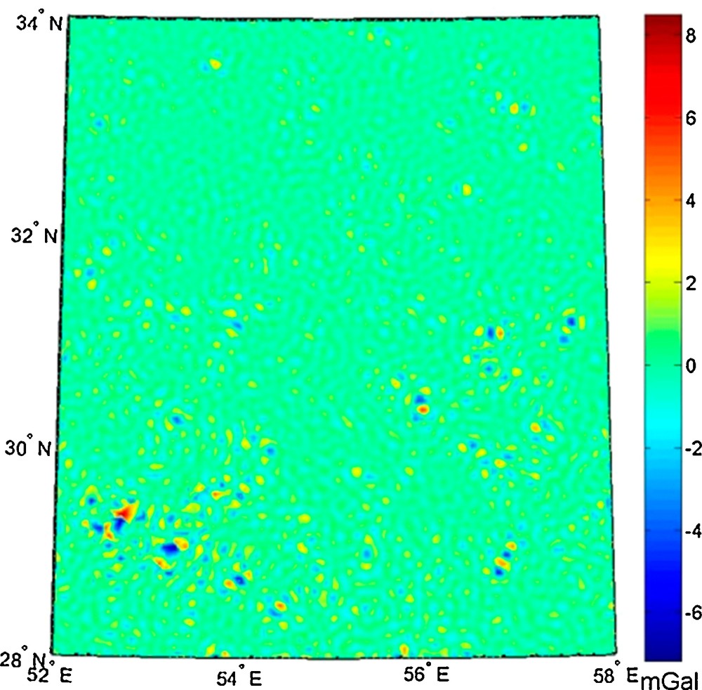
The optimal gravity field and quasi-geoid modeling with RBFs is investigated based on the proposed data processing scheme and on the modifications applied to the Levenberg–Marquardt algorithm. The study area is situated between 52° < λ < 58° and 28° < φ < 34° in Iran. The topographic heights are retrieved from the ACE2 Global Digital Elevation Model (SRTM 2) dataset with a spatial resolution of 2.5 × 2.5 arcmin. The topographic heights at the study area vary from 152.56 to 3963.09 m (Fig. 1). The gravimetric dataset consists of 21,006 synthetic surface gravity anomalies computed with a spectral resolution complete to degree/order of 2160 using the EGM2008 harmonic coefficients. The residual gravity anomalies are obtained after removing the long-wavelength part of the gravity field from the original data (see Fig. 2). The reference gravity field is computed up to degree/order of 360 using the same geo-potential model. All the residual gravity anomalies are disturbed by the white Gaussian noise with the STD of about 0.5 mGal. Nine hundred and seventy-six independent points are considered as the gravity control points for the implementation of RMS minimization technique and avoiding over-parameterization. In addition, the gravimetric height anomalies at 40 independent points are synthesized using the EGM2008 up to degree/order of 2160. These height anomalies are used to evaluate the accuracy of the gravimetric quasi-geoid model parameterized by RBFs.

Fig. 1
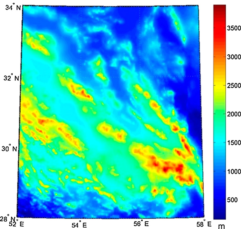
Topographic map of the study area.

Fig. 2
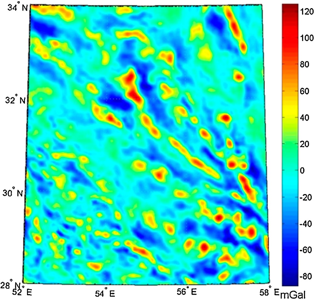
Residual gravity anomaly map of the study area.

Due to numerical simplicity of the Newtonian point-mass kernel for gravitational potential, this kernel is chosen as RBF to investigate the capability of the proposed methodology. The analytical form of point-mass kernel is expressed as follows (Wittwer, 2009):

ψ (x, y_{n}) = \frac{1}{|x - y_{n}|}

(10)

where

|x - y_{n}|

is the Euclidean distance between the observation point x and the nth point-mass y_n. In the spherical coordinate system, this Euclidean distance is defined as follows (Lin et al., 2014):

|x - y_{n}| = \sqrt{{|x|}^{2} + {|y_{n}|}^{2} - 2 |x| |y_{n}| \cos θ}

(11)

where θ is the spherical distance between the observation point and point-mass that is defined as:

\cos θ = \sin φ \sin φ_{n} + \cos φ \cos φ_{n} \cos (λ - λ_{n})

(12)

where

(|x|, φ, λ)

is the spherical coordinates of the observation point (radius, latitude and longitude), and

(φ_{n}, λ_{n})

is the center and

|y_{n}|

is the bandwidth of RBF localized at the nth point-mass.

In order to solve the non-linear problem of gravity field modeling parameterized with RBFs, the unknown parameters are initialized as follows:

• RBF centers: the positions of the RBF centres depend on the size of the study area, the spectral content of gravimetric data, the distribution and density of the observations. For a homogeneous data distribution, the initial locations of RBF centres can be set in an equiangular grid network;
• RBF bandwidths or depths: the depths of RBFs depend on the type of RBFs, the horizontal configuration of RBFs, the spectral content of gravimetric data and the variation of topographic heights. Larger depths are expected for the coarser RBF grids. Areas with high altitudes that have high-frequency signal variations can be recovered by localizing smaller depths. The numerical experiments show that the accuracy of the gravimetric models depends on the choice of the initial values of the depths. For a specific RBF network, depths vary less than several millimeters during the iterative optimization procedure. The initial values of the RBF depths can be considered the same and chosen based on the RMS minimization technique (Tenzer and Klees, 2008). In this method, the RMS of the differences between the observed and predicted gravity data is computed at the control points. If initial values of the RBF depths are chosen properly, the minimum RMS is obtained at these control points. In this study, the proper initial value of the depth is about 6.5 km below the Bjerhammar sphere;
• Scaling coefficients: these parameters specify the magnitude and contribution of each RBF in the recovery of gravity observations. If the initial 3D positions of RBFs are chosen, the initial values of the scaling coefficients can be determined using a linear least-squares adjustment.

The data processing scheme starts with a coarse grid network of RBFs with the 10 arcmin grid size consisting of 1369 base functions. Then, the RBF grid is gradually made denser. Due to the modifications applied to the optimization algorithm, the number of iterations reduces significantly and all the results are obtained after at most 33 iterations (Table 1). Based on the designed data processing strategy, it is expected that adding more RBFs yields smaller values of $σ_{k}^{2}$ in Eq. (8), but after selecting a specific number of RBFs, adding more RBFs causes this quantity to start to increase. This specific number of RBFs corresponds to the optimal number of base functions and optimal RBF parameters. As seen in Fig. 3 (see also Table 1), a network of 1764 RBFs provides the optimal solution. In order to validate the results of the proposed approach, it is compared to the existing methods. Based on the trial-and-error approach proposed by Safari et al. (2014), the minimum RMS of residual height anomalies is the result of an optimal number of RBFs. Fig. 4 shows the RMS of residual height anomalies as a function of the number of RBFs. The corresponding numerical results are shown in Table 1. As can be seen, the use of 1764 RBFs gives the minimum RMS at the height control points. Therefore, the reliability of the proposed optimization methodology is confirmed by the approach of Safari et al. (2014). An important advantage of the proposed methodology is, however, that the validation of the parameterized gravity field model does not require different types of data, namely the GPS/Leveling information. If we define the least-squares residual gravity anomaly as the difference between the observed and predicted residual gravity anomalies with RBFs, it can be seen that after selecting the optimal number of RBFs, adding more RBFs has no significant effect on the RMS of the least-squares residuals, and the RMS changes are less than 0.1 mGal (see Fig. 5 and Table 1). Based on the optimal solution, the residual gravity anomalies are approximated with the accuracy of 0.9 mGal. The least-squares residual gravity anomaly map is presented in Fig. 6. The gravimetric quasi-geoid model is determined with the accuracy of 2.2 cm at the height control points, and no-significant bias is observed in these points (Table 2). The gravimetric quasi-geoid model of the study area is shown in Fig. 7.

No. of RBFs	1369	1444	1521	1600	1764	1849	1936	2025	2116	2209	2304
No. of iterations	28	32	33	29	31	32	32	33	28	31	29
$σ^{2}$ (×10⁻⁶)	12.730	6.546	0.727	0.382	0.026	0.081	0.194	0.477	0.606	0.869	2.302
RMS of residual height anomalies (m)	0.125	0.069	0.066	0.034	0.022	0.043	0.047	0.063	0.066	0.072	0.075
RMS of least-squares residual gravity anomalies (mGal)	5.103	3.147	1.953	1.366	0.901	0.842	0.792	0.773	0.740	0.710	0.671

Fig. 3
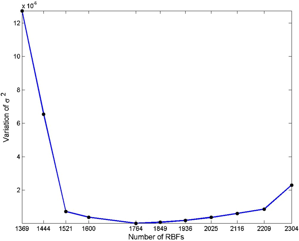
Variation of $σ_{k}^{2}$ as a function of the number of RBFs.

Fig. 4
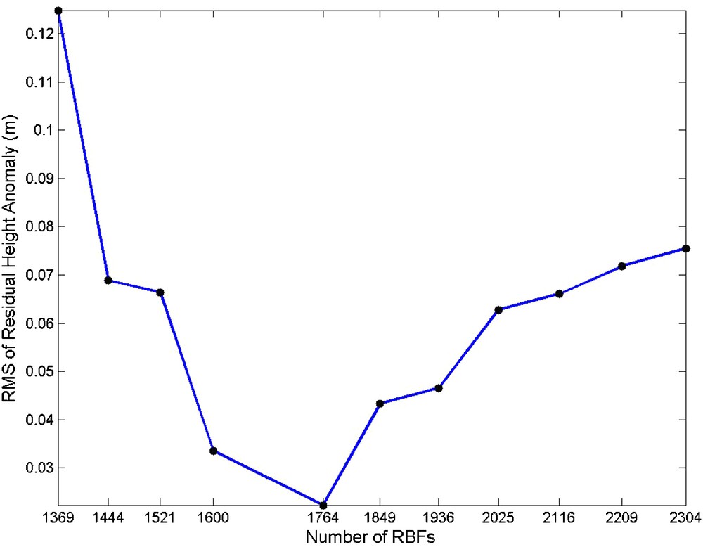
RMS of residual height anomalies (m) as a function of the number of RBFs.

Fig. 5
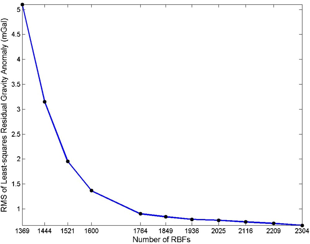
RMS of least-squares residual gravity anomalies (mGal) as a function of the number of RBFs.

Fig. 6
Least-squares residual gravity anomalies (mGal); min = –7.44, max = 8.73, mean = –0.0005, STD = 0.901.

	Min	Max	Mean	STD
Quasi-geoid height (m)	–17.130	–2.980	–8.943	3.994
Height anomalies modeled using RBFs (m)	–17.101	–2.918	–8.928	3.993
Residual height anomalies (m)	–0.092	0.017	–0.016	0.022

Fig. 7
Gravimetric quasi-geoid model of the study area (m).

6 Summary and conclusion remarks

In order to optimize the non-linear problem of gravity field and quasi-geoid modeling with RBFs, we designed a specific data processing scheme using the Levenberg–Marquardt algorithm as the regularization method. Due to the simplicity of the point-mass kernel, this kernel was chosen as RBF to investigate the performance of the proposed strategy. In order to improve the performance of the designed processing scheme, we considered some issues: two modifications were applied to the Levenberg–Marquardt algorithm, and proper initial values of RBF parameters were provided. We modified the Levenberg–Marquardt algorithm through suggesting a novel formula to initialize the regularization parameter, and proposing a specific updating rule for this parameter. Proper initial values of the RBF centres were selected in an equiangular grid. The RBF bandwidths were initialized based on the RMS minimization technique, in which the minimum RMS of least-squares residual gravity anomalies at control points is the result of properly selected depths. Considering the initial values of the 3D positions of RBFs, the initial values of scaling coefficients were determined by applying a linear least-squares adjustment. The reliability of the proposed data processing strategy was confirmed with previous methods for finding the best number of RBFs. Finally, we found the regional gravity field model with a standard deviation of 0.9 mGal, and the gravimetric quasi-geoid model with a standard deviation of 2.2 cm.

Compared to the previous methods, some of the most important advantages of the methodology proposed in this study are that:

• we found that 8.4% is the ratio between the number of RBFs and the number of observations in our study area, which comprises a rough mountain terrain. This low number of applied RBFs improved the time efficiency of computations significantly;
• we provided a novel approach to initializing the RBF and regularization parameters. Therefore, the probability of convergence of the solution to the global minimum was enhanced while reducing the number of iterations significantly, and thus, increasing numerical efficiency;
• we proposed a reliable validation technique based on our data processing scheme in which the gravimetric quasi-geoid model is validated without requiring any external information about the Earth's geoid, such as the GPS/leveling data that might not be always available.

Bibliographie

[Barthelmes and Dietrich, 1991] F. Barthelmes; R. Dietrich Use of point masses on optimized positions for the approximation of the gravity field, Int. Assoc. Geod. Symp., Volume 106 (1991), pp. 484-493

[Engl and Kugler, 2005] H. Engl; P. Kugler Nonlinear inverse problems, theoretical aspects and some industrial applications, Math. Indust., Volume 6 (2005), pp. 3-47

[Foroughi and Tenzer, 2014] I. Foroughi; R. Tenzer Assessment of the Direct Inversion Scheme for the Quasigeoid Modeling based on applying the Levenberg–Marquardt algorithm, Appl. Geomatics, Volume 6 (2014), pp. 171-180

[Foroughi et al., 2013] I. Foroughi; R. Tenzer; A. Safari Application of the Levenberg–Marquardt Algorithm in Local Gravity Field Modeling using Radial Basis Functions, Proc. IAG Scientific Assembly, GFZ German Research Centre for Geosciences, 2013

[Gavin, 2013] H.P. Gavin The Levenberg–Marquardt method for nonlinear least squares curve fitting problems, Department of Civil and Environmental Engineering Duke University, 2013

[Hardy and Göpfert, 1975] R. Hardy; W. Göpfert Least squares prediction of gravity anomalies, geoidal undulations, and deflections of the vertical with multiquadric harmonic functions, Geophys. Res. Lett., Volume 2 (1975), pp. 423-426

[Klees et al., 2008] R. Klees; R. Tenzer; I. Prutkin; T. Wittwer A data-driven approach to local gravity field modeling, J. Geod., Volume 82 (2008), pp. 457-471

[Klees and Wittwer, 2007] R. Klees; T. Wittwer A Data-adaptive design of a spherical basis function network for gravity field modeling. Dynamic planet, International Association of Geodesy Symposia, 2007, p. 130

[Lin et al., 2014] M. Lin; H. Denker; J. Muller Regional gravity field modelling using free positioned point mass, Stud. Geophys. Geod., Volume 58 (2014), pp. 207-226

[Marchenko, 1998] A.N. Marchenko Parameterization of the Earth's gravity field. Point and line singularities, Lviv Astronomical and Geodetic Society, 1998

[Marquardt, 1963] D.W. Marquardt An algorithm for least squares estimation of nonlinear parameters, J. Soc. Ind. Appl. Math., Volume 11 (1963), pp. 431-441

[Moritz, 1980] H. Moritz Advanced Physical Geodesy, Abacus Press Tunbridge Wells Kent, 1980

[Ortega and Rheinboldt, 1970] J. Ortega; W. Rheinboldt Iterative Solution of Nonlinear Equations in Several Variables, Academic Press, New York and London, 1970

[Safari et al., 2014] A. Safari; M.A. Sharifi; H. Amin; I. Foroughi; R. Tenzer Determining the Gravitational Gradient Tensor Using Satellite-Altimetry Observations over the Persian Gulf, Mar. Geod., Volume 37 (2014), pp. 404-418

[Tenzer and Klees, 2008] R. Tenzer; R. Klees The choice of the Spherical Radial Basis Functions in Local Gravity Field Modelling, Stud. Geophys. Geod., Volume 52 (2008), pp. 287-304

[Tenzer et al., 2012] R. Tenzer; R. Klees; T. Wittwer Local Gravity Field Modeling in Rugged Terrain Using Spherical Radial Basis Functions: Case Study for the Canadian Rocky Mountains, Geod. Planet Earth Int. Assoc. Geod. Symp., Volume 136 (2012), pp. 401-409

[Tyagi, 2011] K. Tyagi Second Order Training Algorithms For Radial Basis Function Neural Network, The University of Texas, 2011

[Weigelt et al., 2010] M. Weigelt; M. Antoni; W. Keller Regional Gravity Field Recovery from GRACE Using Position Optimized Radial Base Functions. Gravity, Geoid and Earth Observation, Int. Assoc. Geod. Symp., Volume 135 (2010), pp. 139-146

[Wittwer, 2009] T. Wittwer Regional Gravity Field Modelling With Radial Basis Functions, Delft University, The Netherlands Geodetic Commission, 2009

Commentaires - Politique

Ces articles pourraient vous intéresser

Local gravity field modeling using spherical radial basis functions and a genetic algorithm

Hany Mahbuby; Abdolreza Safari; Ismael Foroughi

C. R. Géos (2017)

A transform based local RBF method for 2D linear PDE with Caputo–Fabrizio derivative

Kamran; Amjad Ali; José Francisco Gómez-Aguilar

C. R. Math (2020)

Radial point interpolation method and high-order continuation for solving nonlinear transient heat conduction problems

Said Mesmoudi; Omar Askour; Bouazza Braikat

C. R. Méca (2020)