

1 Introduction
The series of spherical harmonics is the commonly used method for global gravity field modeling; however, Spherical Radial Basis Functions (SRBFs) can locally represent the gravity field of the Earth. The Stokes coefficients of spherical harmonics are sensitive to local signal changes, although SRBFs are often used to model the higher frequencies of the field and can be used as an alternative method for regional modeling of the Earth's gravity field and the corresponding quasigeoid models. The Earth's gravity field can be expressed by a linear combination of the SRBFs (Barthelmes and Dietrich, 1991). The kernels of SRBFs are mostly of the inverse-distance type, which can be defined in different ways; for instance, the point-mass kernel (Barthelmes, 1988; Barthelmes and Dietrich, 1991; Blaha et al., 1986; Lin et al., 2014; Shahbazi et al., 2015; Sünkel, 1981; Weightman, 1965). Later the higher order of point-mass, radial multi-poles, were introduced by Marchenko (1998) and used by Foroughi and Tenzer (2014). Poisson wavelets, were derived by Holschneider et al. (2003) and later used by Chambodut et al. (2005); Klees and Wittwer (2007); Klees et al. (2008); Panet et al. (2006); Safari et al. (2014); and Tenzer et al. (2012). The band-limited Blakman base functions were first used by Schmidt et al. (2004, 2005). Tenzer and Klees (2008) showed that there is no significant difference between different types of kernels when they are parameterized properly.
The parameterization of the gravity field using SRBFs consists in defining the type of kernel, the number of kernels, the location of the center of the kernels, and kernel bandwidths that all have a considerable effect on the predicted model. Using many kernels leads to overparameterization, while applying a low number of them can only represent the low-frequency part of the model. The SRBF kernel is defined on or within the sphere which is completely located inside the Earth's topography and is known as the Bjerhammar sphere (Moritz, 1980). SRBF kernels are typically defined as inverse distances between integration points in the target area and computation points in the data coverage. An inverse relation exists between the kernel's bandwidth and the kernel's depth into the Bjerhammar sphere. Some studies (Klees et al., 2008; Tenzer et al., 2012) consider the depth of the kernels as separate unknown parameters rather than their 2D location. However, the unknown parameters can be merged into 3D positions of the kernels on the Bjerhammar sphere and be found in one step (Shahbazi et al., 2016).
Finding the number of base functions (kernels) and the location of their centers is the first step of SRBF parameterization. Different methods have been proposed to find the optimum number with respect to the location of the observation points and the depth of kernels into the Bjerhammar sphere. Marchenko (1998) used radial multi-pole kernels below the observation points and then optimized the solution using a sequential multi-pole algorithm. The depth and order of the radial multi-pole kernels were then determined by the covariance function of the signal around the observation points. Klees and Wittwer (2007) and Klees et al. (2008) proposed a methodology that was fully based on the distribution of the data. They used an initial regular grid of the SRBFs to carry out the first adjustment; then they added local base functions to the areas where the residuals between observation and predicted anomalies were larger than a predefined tolerance. The generalized cross-validation method was also applied to approximate the optimal depth. Their method was only applicable in areas with dense gravity data coverage and smooth topography. Tenzer et al. (2012) analyzed the least squares approximation of the gravity field via Poisson wavelets of order 3 on various spherical equiangular grids, and they used the method of minimization of the RMS differences between predicted and observed gravity disturbances to find the optimal depth of the kernels. They reduced the number of the required base functions by applying topographical corrections. Foroughi and Tenzer (2014) introduced the Levenberg–Marquardt algorithm to minimize the number of base functions and find their depth based on Least Square (LS) adjustment; they suggested the use of a two-step process to find the optimal number of base functions. In the first step, the optimum number of base functions was defined based on the fitting between observed and predicted gravity anomalies and in the second step the optimum number was chosen according to best fitting between observed and predicted quasigeoidal heights. The common optimum number between the two steps was then selected as the number of kernels. The two-step method did not require adding extra local kernels manually, but it was computationally expensive and needed independent control points with two types of observations: gravity anomalies and normal heights. Later Shahbazi et al. (2016) modified this method so that the number of base functions could be chosen in one step. Their method allows one to find the optimum number based on estimated errors in the observation data as well as their distribution.
The proposed methods of parameterization of SRBFs in previous studies are limited to the initial choice of the location and depth of the kernels and some are not able to choose the number of kernels automatically. These methods might represent the “local minimum” of the parameterized solution because their final solution does not differ significantly from their initial values. They mostly use corrector surfaces to fit the final gravity model to local GNSS/Leveling data points, which simply hides the discrepancies between the predicted and the observed model. The intention of the current study is to employ the Genetic Algorithm” (GA) and let the parameters of the kernel of SRBFs be chosen based on the information provided in the observation data. The proposed method in this study can search among all the possible solutions of parameterized SRBFs and find the “global minimum” of the target function that is set to be minimized in the process. Once the parameters of SRBFs are found using GA, the system of linear equation, in the LS sense, is solved based on the Conjugate-Gradient (CG) technique, which leads to an un-biased solution, unlike the previously used approaches.
The theory of SRBFs in gravity field modeling is described in Section 2. General information on GA is provided in Section 3.1. The iterative approach of CG is presented in Section 3.2. The methodology of problem solving is explained in Section 4. The numerical results and discussion are touched on in Section 5 and Section 6, respectively. At the end, Section 7 summarizes the remarks of this contribution.
2 Theory of regional gravity field modeling using SRBFs
According to the Runge–Krarup theorem, a harmonic function can be regarded as an expansion of the non-orthogonal base functions. The disturbing potential of the Earth's gravity field is considered harmonic above the geoid (Moritz, 1980), therefore, we can represent it as a linear combination of the set of non-orthogonal base functions (Marchenko, 1998):
| (1) |
| (2) |
| (3) |
| (4) |
Eq. (3) can be parameterized with the system of linear equations where the gravity anomalies are observations and the unknown parameters consist of the location of the kernel's center, the kernel's depths, and scale coefficients.
3 Optimization of the SRBFs via genetic algorithm
3.1 Genetic algorithm
The Genetic Algorithm (GA) technique was first introduced by Holland (1975) who established a method to find the optimal solution of an optimization problem based on artificial intelligence. In this problem, a “target function” (or fitness function) is defined by the user to be minimized or maximized, depending on its definition, during the process. “Genes” are considered the unknown parameters and each set of genes is placed in one “chromosome”. Hence, each chromosome has the length of the number of unknown parameters. Based on the initial limits of chromosomes, the GA produces an initial population of the solutions which are called “offspring”. The offspring will be produced to optimize the target function and the ones which move towards the optimal solution will be selected as new chromosomes (“parents”) to participate in reproduction. Thus, the evolution process will continue until the point that the chromosomes can no longer produce “better” offspring, i.e. the value of the fitness function is smaller than a specified tolerance (noise of input data). These sets of chromosomes will be considered to be the global optimal solution to the problem (cf. Haupt and Haupt, 2004). To stop the algorithm according to the physical constraints of the problem, a criterion of producing a certain number of generations can be considered. However, the number of iterations can be different according to the choice of initial values which are introduced by the user.
In every iteration, each set of chromosomes will be regarded as one population. Each chromosome has a fitness score that is the inverse of its target function's value. The chromosomes with a higher fitness score will be more involved in the crossover process to produce new generations. During the reproduction, “mutation” will make small changes in the chromosomes (normally between 0.001 and 0.5), to avoid getting the solution trapped in local minimums. The “migration” between populations is in the forward direction, i.e. the chromosomes of population of the nth iteration migrate to the (n + 1)th iteration. To apply the GA, the Matlab original GA toolbox scripts were used and its functions were modified to fit our desired numerical problem (Chipperfield et al., 1994).
3.2 Conjugate gradient least squares method
Conjugate Gradients (CG) is an iterative method to estimate the best solution of an overdetermined badly conditioned Least Square (LS) problem, which we will here call CG–LS. CG–LS simply looks for the unknown parameters (x) where they best satisfy the equation Ax = b (Björck et al., 1988):
| (5) |
| (6) |
| (7) |
| (8) |
The unknown parameters in this algorithm are the scale coefficients (Ci in Eq. (1)).
4 Methodology
The location of base functions on or below the Bjerhammar sphere, as well as their depth, should be defined optimally to predict the local gravity field model; this is a non-linear optimization problem. The scale coefficients are the unknown parameters of a linear problem once the base functions are parameterized (the values of ϕi is known per Eq. (1)). In this study, GA as a non-linear optimization method is combined with CG–LS as a linear regularization method to locally predict the gravity field model. The following flowchart summarizes the combination of these two methods:
In this method, GA is expected to find only the optimal location and depth of kernels and not their numbers. Thus, the length of the chromosomes is fixed in GA and is three times the number of kernels (longitude, latitude, and depth are unknowns). Instead of fix-length chromosomes, variable-length chromosomes can be used. The number of kernels can be considered as an integer unknown parameter along with other unknowns. However, the location of kernels is a function of this number and so the algorithm needs longer time to converge and also the limit which GA is searching to optimize the fitness function is much larger than fix-length chromosome mode. So, to get a faster solution, the number of kernels was set to a fix value. A range of different numbers of base functions should be tried in the algorithm, and the predicted solution in terms of gravity and height anomaly will be compared with observations to find the best number (cf. Foroughi and Tenzer, 2014). Once the number of SRBFs is specified, GA can establish a population of chromosomes with the length of unknown parameters of kernels and their limits. The limit of both longitude and latitude is the data coverage area, and depth is limited between zero (on the Bjerhammar sphere) and 100 km (Klees et al., 2008). The maximum depth of the kernels can be different depending on their type. Choosing a larger limit of depth elongates the process; in our experience the depth typically is not more than 100 km.
The initial location of kernels is a regular grid on the Bjerhammar sphere (where depth is zero) and the grid spacing is defined as follows:
| (9) |
| (10) |
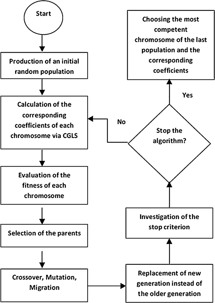
The flowchart of the combination of GA and CG–LS for local gravity field modeling using SRBFs.
The algorithm stops when the value of the fitness function (Eq. (10)) is smaller than the specified tolerance.
5 Numerical study
To evaluate the proposed method, the point-mass kernel was used to locally predict the gravity field of the Auvergne area, which is limited by longitudes of 2.5 to 3.5 degrees and latitudes of 45 to 46 degrees. The topographic heights of the study area are calculated from the DTM2006 model and they vary within the range of 269.8 to 1649.2 m, as shown in Fig. 2. The input data are synthetic surface free-air gravity anomalies and height anomalies (simulated to represent the GNSS/leveling points) which are computed up to the degree and order of 2160 using the EGM2008 model on a 1 × 1 arc-min grid (Pavlis et al., 2012).
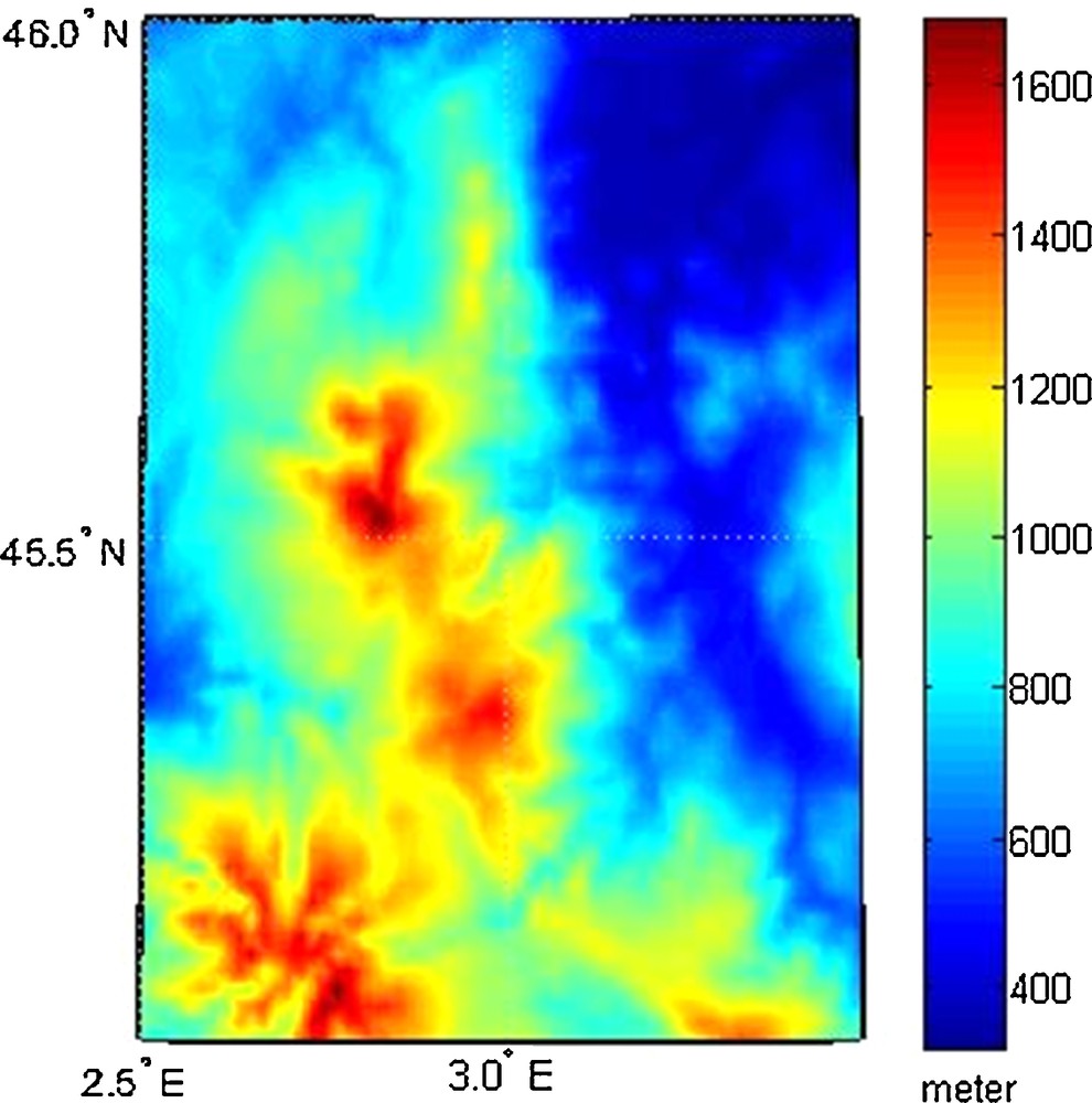
The topography over study area.
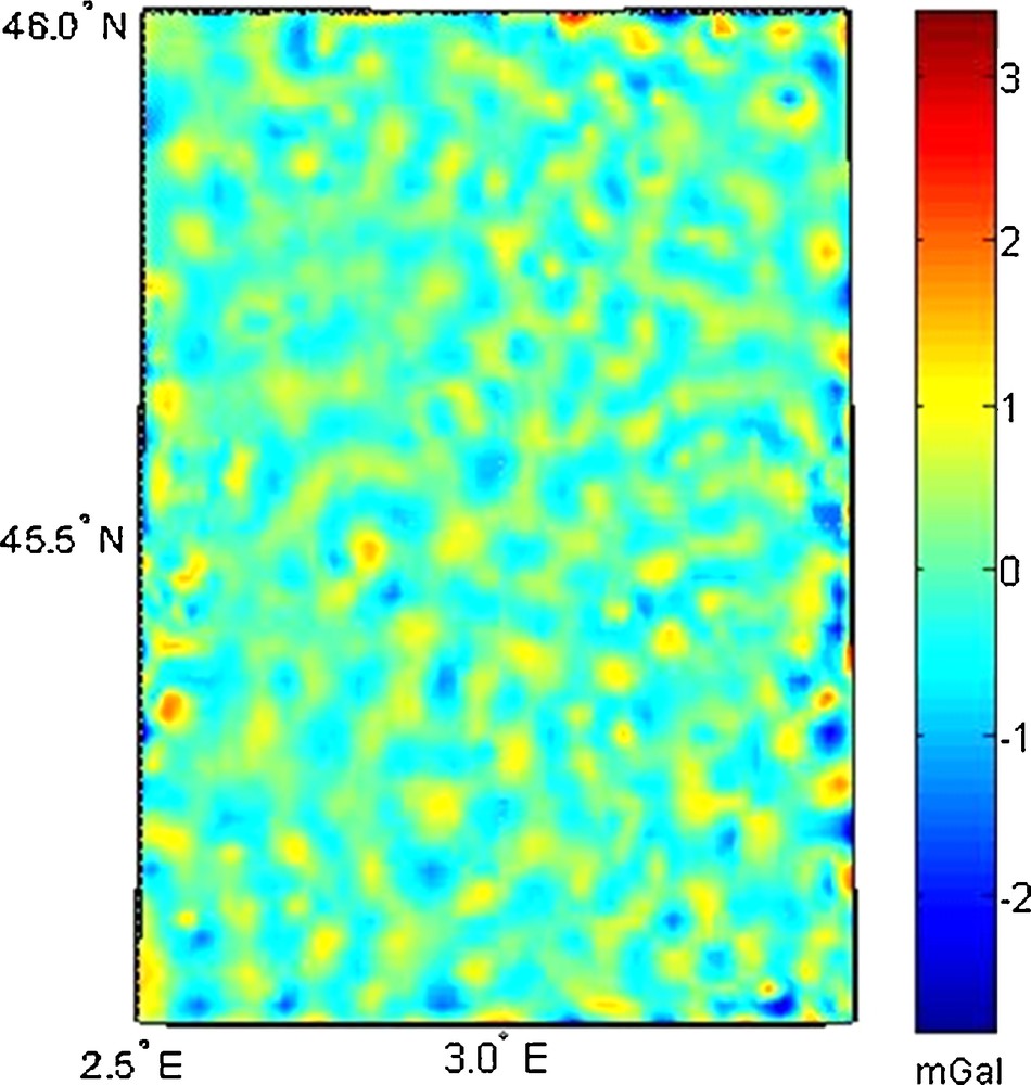
The low-frequency part of gravity anomalies (synthetic anomalies up to the degree and order of 360) were removed from the input gravity anomalies. The residual gravity anomalies were used for gravity field modeling using SRBFs. A white Gaussian noise of 0.5 mGal was also added to input data to get the process closer to reality (Fig. 3).
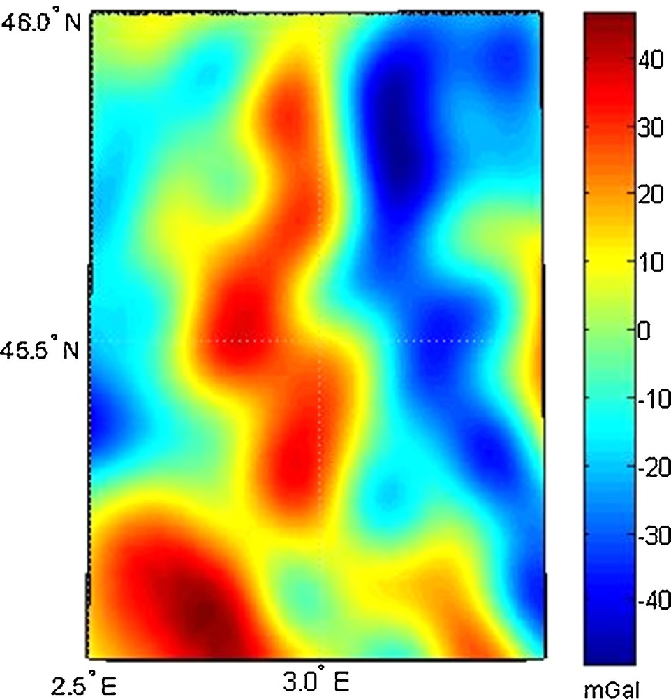
Free-air gravity anomalies over study area.
Although using a large number of SRBFs better predicts the gravity anomaly, it increases the instability of the problem and it might result in a biased solution in height anomalies. It is also computationally more time consuming, even though it does not give a better solution in terms of height anomalies. Pursuant to the two-step method introduced by Foroughi and Tenzer (2014), a limited number of kernels were used in modeling. In this study, a range of 100 mass-point kernels up to 500 with a step of 50 kernels were used for each stage, then the RMS of the differences between predicted and observed gravity and height anomalies were computed (Table 1). To show how the statistics of the residual between predicted and observed gravity and height anomalies react to the number of kernels, the test was done for a maximum of 2000 kernels, and the results are shown in Fig. 4.
Investigation of the RMS of the differences between predicted and observed gravity and height anomalies using different numbers of base functions.
| No of SRBFs | 100 | 150 | 200 | 250 | 300 | 350 | 400 | 450 | 500 |
| RMS of differences between predicted and observed gravity anomalies at observation points (mGal) | 2.62 | 1.54 | 1.33 | 0.89 | 0.59 | 0.38 | 0.35 | 0.23 | 0.2 |
| RMS of differences between predicted and observed height anomalies at GNSS/leveling points (m) | 0.12 | 0.13 | 0.12 | 0.12 | 0.11 | 0.13 | 0.12 | 0.13 | 0.13 |
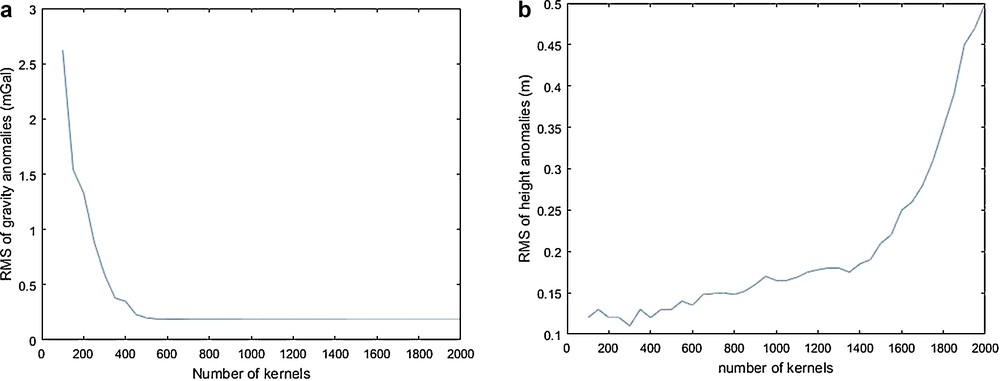
Comparison of RMS of differences between predicted and observed height anomalies to find the optimal number of base functions. a: RMS of the differences between predicted and observed gravity anomalies (mGal) as a function of the number of SRBFs; b: RMS of the differences between predicted and observed height anomalies (m).
Fig. 4a shows that RMS of differences between predicted and observed gravity anomalies decrease with the number of kernels; however, the trend is different with regard to height anomalies (Fig. 4 b). The large RMS value in residuals of height anomaly leads to a biased solution when the number of kernels is set to an unnecessarily large number. Considering this, 300 kernels is the optimal choice and more leads to an overparameterized problem.
The proposed method in Section 4 was used to find the optimal location of kernels. Two hundred and eighty-nine kernels were located on a regular grid in the data coverage area, i.e. there were 17 kernels along both the latitude and longitude sides (cf. Eq. (9)). Five percent of the input data were removed as independent control points, and 0.5 mGal of RMS of differences between predicted gravity anomalies and height anomalies on these points were used to stop the iterations. The iteration stopped after 1503 iterations, and the optimal SRBF parameterization was used to predict the residual gravity and height anomalies. The computation time using a 64-bit operation system including 8.00 Gb of RAM and 8 core of 3.7 GHz CPU was 3 h and 32 min. The average estimation of the depth of each kernel was 17.3 km below the Bjerhammar sphere, and the kernels were mostly located in high topographical areas (Fig. 5). The RMSs of 0.48 (mGal) and of 0.09 (m) were achieved for predicted gravity anomalies and height anomalies, respectively. The residuals have a random distribution and do not show any bias (Fig. 6).
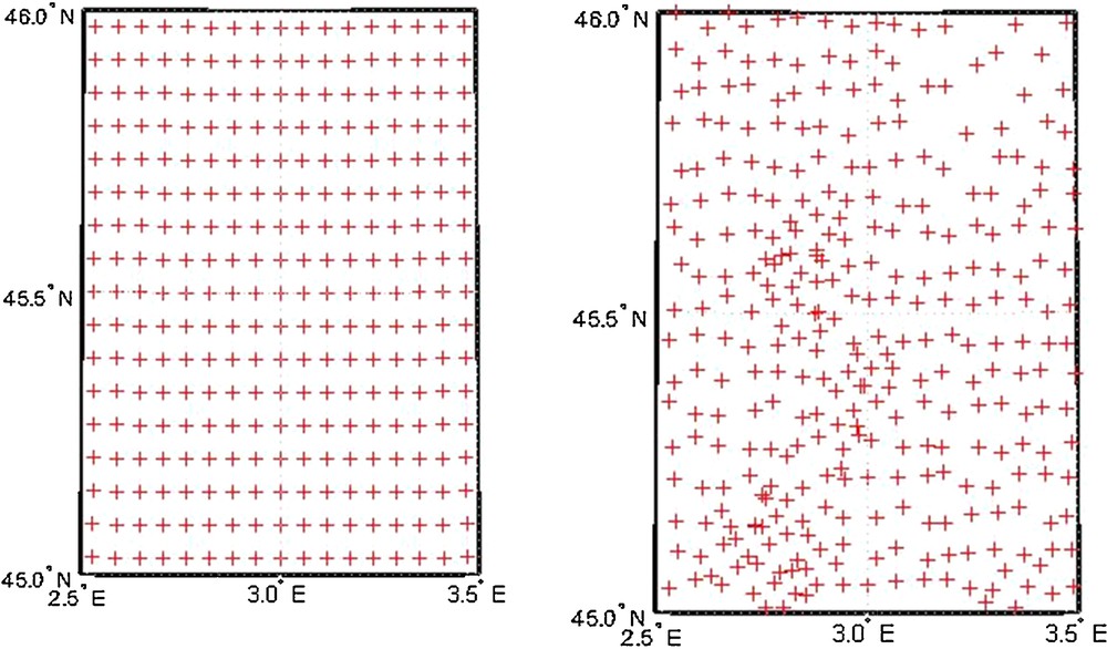
The movement of the location of kernels during the GA process. a: the initial location of kernels on regular grid; b: the optimal location of kernels after optimization.
The residuals between predicted and observed gravity anomalies.
6 Discussion
The GA along with the CG–LS method was used to find the optimal location of SRBF's kernels and scale coefficients in the parameterization of local gravity field modeling. Point-mass type of kernels was used to predict the synthetic gravity anomalies on a 1 × 1 arc-min grid in a rough topographical area of Auvergne. The number of kernels, and their longitude, latitude, and depth inside the Bjerhammar sphere were limited based on physical constraints of the gravity model in GA. The RMS of the predicted height anomaly on control points manages the number of kernels to prevent overparameterization. The fitness function for the evaluation of the chromosomes was defined such that predicted gravity anomalies shows the best conformity with the observation points in the RMS sense. The CG–LS method was applied to find preliminary scale coefficients before the evaluation of the chromosomes and was updated for each population in GA. The number of iterations of this technique was set to reduce the value of the target function to less than the specified tolerance. The convergence of the fitness function with respect to the number of iteration is shown in Fig. 7. Two hundred and eighty-nine kernels were used in the GA algorithm and around 1500 iterations were needed to achieve the desired accuracy.
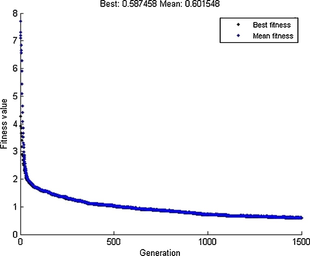
The convergence of the GA to find the optimal location of kernels.
7 Conclusion
The Genetic Algorithm was applied to regional gravity field modeling using Spherical Radial Basis Functions. Gravity anomaly and quasigeoid models can be computed using predicted models in the area of interest. The ability to optimize the positions of the base functions efficiently was the main advantage of using GA. Results showed that kernel centers and their depth do not necessarily need to be fixed. The depth or bandwidth of each kernel can be different and is computed by combining with the 3D location of the kernel. Results also revealed that with a small number of kernels the gravity model can be regionally predicted bias-free. The determination of the appropriate parameters for the crossover, mutation, and migration processes is an important point that should be considered for better application of this method. The proposed method can build the most adapted model with data for any arbitrary number of kernels; however, large numbers of kernels might need longer processing times and can produce large biases in predicting the height anomalies.