

1 Introduction
The surface temperature averaged over the whole globe has unequivocally increased over the last century (IPCC, 2013). It is plotted in Fig. 1, using the HadCRUT4 compilation (Morice et al., 2012) for illustration. There is nevertheless substantial variability around the very clear positive trend over the period 1870–2015, with decades of accelerated increase and others of decreasing tendencies. These decadal fluctuations are primarily the manifestation of the natural variability, which is related to the effect of natural external forcing of the climate system, like solar irradiance variations and volcanic eruptions, as well as to the intrinsic variability of the ocean–atmosphere–ice coupled system. The climate system indeed fluctuates, even if external forcing does not vary.
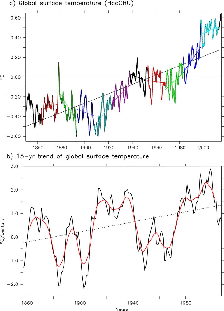
(a) Monthly mean of global surface temperature anomalies (reference period is the whole period) from HadCRUT4 until May 2015. (b) Fifteen-year trend since 1850 from HadCRU data using a one-year sliding window to compute the linear trend from monthly mean data. The red line in (b) is a three-year running mean of the black line.
The anthropogenic forcing of the climate system, mainly associated with greenhouse gas concentrations and aerosols emissions, is evolving very smoothly (Fig. 2). It can thus hardly explain such decadal fluctuations, except maybe for the rapid increase in aerosols release at the beginning of the 1960s, which may partly explain the cooling experienced at that moment (Stott et al., 2000), as well as the increase in aerosols emissions in Asia from the 1990s, which may induce complex teleconnection patterns (Smith et al., 2016). Natural variability otherwise remains the main candidate for explaining the decadal fluctuations occurring on top of the long-term warming trend.
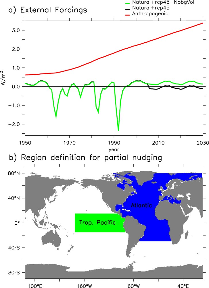
(a) External forcing applied in the different simulations (see Table 1), and (b) definition of the region where partial nudging has been applied (tropical East Pacific in green, Atlantic in blue).
The period between ∼1998 and ∼2012 experienced a particularly weak warming trend as compared to the preceding decades, while the anthropogenic forcing was as strong as during the previous decade, if not stronger. This event has been dubbed as a hiatus, given that the simple direct response to anthropogenic increase in greenhouse gases emissions should have been a quasi-linear warming over the last 30 years. Many studies have tried to attribute it either to natural variability or to anthropogenic aerosols emissions. In this sense, this fluctuation has been a stimulating test bed to evaluate our level of understanding of the sources of fluctuations of the climate system.
Several interesting hypotheses have emerged to explain this hiatus period. Santer et al. (2014) have proposed that the accumulation of small (tropospheric) volcanic eruptions over this period has led to a significant loading of aerosols in the atmosphere, which has increased its albedo and thus reflected a large amount of solar short-wave radiation. This effect may have mitigated the Earth surface temperature increase due to the increase in greenhouse gases concentrations in the atmosphere. In addition to this natural fluctuation in the external forcing, other analyses have scrutinized the specific spatial pattern of the temperature changes over this time period (Kaufmann et al., 2011; Kosaka and Xie, 2013). They have highlighted the fact that the Pacific basin, which accounts for more than a third of the Earth surface, has experienced a cooling trend in the 2000s in many locations, following a pattern resembling a well-known mode of decadal variability in this basin, the so-called Pacific Decadal Oscillation (PDO, Mantua et al., 1997). Meehl et al. (2011) showed that, in climate models projections of the 21st century, periods with small decadal warming trends are typically characterized by a negative phase of the PDO. Indeed, during such phases, the equatorial upwelling of cold deep water is enhanced, while warm waters from the western warm pool subduct. Consequently, the additionnal heat received in the Earth system due to increased greenhouse effect is buried in subsurface, while the deeper ocean is providing cold water at the surface, which cools a large part of the upper Pacific basin (Balmaseda et al., 2013; Douville et al., 2015). This specific state in the Pacific Ocean in the 2000s has been related with abnormally strong easterly winds in the western part of the tropical Pacific Ocean, which may ultimatly explain the adjustment of this basin (England et al., 2014) and the negative phase of the PDO. Nevertheless, the origin of this extreme anomalous wind remains unknown.
Kosaka and Xie (2013) have shown that restoring a climate model towards the observed sea surface temperature (SST) trend in a small region of the eastern equatorial Pacific only representing 8.2% of the Earth surface is sufficient to reproduce most of the spatial features of the anomalies of the hiatus period over the whole Pacific, including wind variations. Indeed, the change in the zonal temperature gradient of the tropical basin activates the Bjerknes feedback, a mechanism by which the east–west SST gradient in the tropical area drives the surface winds, which then feed back positively on the temperature gradient. Furthermore, the associated modification of the Walker cell, the zonal longitude-altitude atmospheric large-scale rotating tropical cell, can also impact the deep atmospheric convection zone in the western Pacific. This provides a vorticity source to excite Rossby waves, that lead to teleconnection patterns towards the high latitudes. This notably explains the cooling pattern observed in the Northeast Pacific during the hiatus (similarly to what happens during a La Niña event). Kosaka and Xie (2013) thus showed that activating a key aspect of this chain of coupled mechanisms can be sufficient to reproduce most of the observed pattern. In this context, a continuum of stochastic perturbations of the wind field fed by teleconnection and then oceanic adjustment in the high latitudes can be sufficient to induce low-frequency variability in the Pacific basin (Newman et al., 2016).
Another idea that has been proposed to explain the increase of easterly wind in the Pacific is based on inter-oceanic basin interactions in the tropical band. McGregor et al. (2014) argued that the Pacific basin may have been influenced by the large warming experienced in the tropical Atlantic in the 2000s, which would have strongly increased the atmospheric deep convection over the Atlantic Ocean, and thereby modified remotely the Walker circulation over the Pacific. Nevertheless, the experimental design they used to test this hypothesis was based on atmospheric-only model simulations or simulations partially coupled with a mixed layer oceanic model. These simplifications may significantly affect the exact representation of the mechanisms at play, and notably the ocean-atmosphere coupling at the root of these mechanisms. Thus, while McGregor et al. (2014) argued that the Atlantic could be the general pacemaker of the multidecadal variability over the globe, Trenberth et al. (2014) showed that variations in the Pacific Ocean could also very well impact the Atlantic Ocean, notably through Rossby waves, highlighting the inherent coupling between the different basins.
Finally, Smith et al. (2016) recently showed that the hiatus period was also related to the delayed recovery of the climate system from the eruption of Mount Pinatubo that occurred in 1991, and to the more recent effect of regional changes in the distribution of anthropogenic aerosols which likely influenced the PDO (see Takahashi and Watanabe, 2016).
Some of the different sources of multidecadal variability described above have been shown to add up in order to quantitatively represent the recent hiatus (Huber and Knutti, 2014; Marotzke and Forster, 2014), but the exact origin of the Pacific variations is still not clear and requires further analysis to decipher and quantify the best hypotheses to explain it.
In this paper, we attempt to reproduce the hiatus characteristics using classical nudging techniques of SST anomalies applied in various versions, and using different representations of the external forcing in the IPSL–CM5A–LR model. This allows us to evaluate the robustness of the different mechanisms proposed to explain the hiatus period in an independent state-of-the-art climate model.
2 Data, model and methods
2.1 Description of the model
The ocean–atmosphere coupled model used in this study is the IPSL-CM5A (Dufresne et al., 2013) in its low-resolution (LR) version as developed for CMIP5. The atmospheric model is LMDZ5 (Hourdin et al., 2006) with a 96 × 96 × L39 regular grid (horizontal resolution around 2.5° in latitude and 3.75 in longitude) and the oceanic model is NEMO (Madec, 2008) with an 182 × 149 × L31 non-regular grid (horizontal resolution around 2°, with refinement up to 0.5° notably at the equator), in version 3.2, including the LIM-2 sea ice model (Fichefet and Morales Maqueda, 1997) and the PISCES (Aumont and Bopp, 2006) module for oceanic biogeochemistry.
2.2 Simulations
The historical simulations use a prescribed external radiative forcing deduced from the observed increase in greenhouse gases and aerosol concentrations as well as the ozone changes (Fig. 2a) and the land-use modifications (not shown, see Dufresne et al., 2013). They also include estimates of solar irradiance variations and of tropical stratospheric volcanic eruptions, represented as a decrease in the total solar irradiance (depending on the intensity of the volcanic eruptions, Fig. 2a, cf. Dufresne et al., 2013), over the historical period, here defined as [1850–2005]. We have run an ensemble of five historical simulations, differing by their initial conditions, taken from different dates of a 1000-year control simulation under pre-industrial conditions, each separated by 10 years. This control pre-industrial simulation is itself starting after thousands of years of spin-up procedure.
Each historical simulation is extended after 2005 following a RCP4.5 emission scenario. These simulations are projections aiming at evaluating the potential impact of future anthropogenic emissions on climate until 2100. To account for possible future volcanic eruptions, which may cool the climate, a constant background volcanic forcing has been added to the external forcing starting in year 2006. It represents the average of volcanic forcing over the period 1860–2000, and is equal to −0.25 W/m2 of global radiative forcing. This anomalous forcing due to background volcanic eruption is not aimed to be realistic on the 2006–2012 period and does not include any information on the timing of the observed forcing effect from volcanic eruptions over this time frame, as described in Santer et al. (2014). Nevertheless, the cumulative radiative forcing over the analysed period is of the same order of magnitude, since Santer et al. (2014) evaluated the radiative impact of tropical eruptions to be around 0.25 W/m2 per decade for a trend computed over January 2001 to December 2012. The historical plus RCP45 scenario including background volcanic forcing ensemble is called HisRbg in the following (cf. Table 1) and comprises five members. These are the historical simulations that have been included in the CMIP5 database. To test the effect of the recent weak volcanic eruptions on the climate variability, and also the effect of the artificial shift of radiative forcing of −0.25 W/m2 imposed in 2006, we have also performed RCP4.5 simulations where the background volcanic eruptions are not considered, named HisRnobg (cf. Table 1).
Description of the five-member ensemble simulations.
| Simulations | Name | Period | Forcing | Restoring |
| Historical + rcp45 without bg Vol. | HisRnobg | 1850–2030 | All but background volcanic eruptions from 2006 | No |
| Nudged Glob. | NudGlo | 1949–2015 | All but background volcanic eruptions from 2006 | Global SST |
| Nudged Pac. | NudPac | 1991–2012 | All but background volcanic eruptions from 2006 | Tropical East Pacific SST |
| Nudged Atl. | NudAtl | 1991–2012 | All but background volcanic eruptions from 2006 | Whole Atlantic |
| Historical +rcp45 with bg Vol. | HisRbg | 1850–2030 | All including background volcanic eruptions in 2006 | No |
The five-member ensemble of nudged simulations over the whole ocean (except below sea ice), called NudGlo, has the same forcing as HisRnobg, and includes a nudging term towards the observed anomalous monthly SST (Smith et al., 2008). Each simulation starts on the 1st of January 1949 from one of the historical simulations presented above (Fig. 2). The nudging technique consists in adding a heat flux term Q to the SST equation under the form Q = −γ (SST’mod−SST’obs), where SST’mod stands for the modelled anomalous SST at each time step and grid point, and SST’obs for the anomalous observed SST (Smith et al., 2008). Anomalies are computed with respect to the monthly climatology of SST over the period 1949–2005 in the corresponding historical simulation and in the observations, respectively. We use a restoring coefficient γ of 40 W·m−2·K−1 corresponding to a physically based (Frankignoul and Kestenare, 2002) relaxing timescale of around 60 days over a 50 m-deep mixed layer (see Swingedouw et al., 2013 or Ortega et al., 2017 for further details). Stronger values of γ, as used in many other studies (Keenlyside et al., 2008; Kosaka et and Xie, 2013; Luo et al., 2005; Pohlmann et al., 2009) have the potential to distort the higher-frequency ocean–atmosphere interaction (Cassou, pers. comm.) or to create spurious water masses in the ocean. In that sense, this study allows the evaluation of new model results obtained with this choice of γ as will be used in upcoming intercomparison projects (cf. Boer et al., 2016).
We also consider partially nudged simulations where we use similar experimental setup as in NudGlo, but imposing the restoring only in limited oceanic areas. We first perform a similar experiment as Kosaka and Xie (2013), where SST nudging is only applied in the tropical East Pacific (called NudPac). The restoring constant used here (40 W·m−2·K−1, as in NudgGlo) is nevertheless six times lower than the one used in Kosaka and Xie (2013). To evaluate the potential impact of the Atlantic basin, we also produce simulations (called NudAtl) with similar external forcing and partial nudging, but only applied in the Atlantic basin (cf. Fig. 2b). Both NudPac and NudAtl types of simulations are mainly designed to reproduce the hiatus period. Therefore, they start in 1990 from global nudged simulations. The area of the Earth surface concerned by the restoring term in the different experiment is around 70% of the globe in NudGlo, 8% in NudPac and 15% in NudAtl.
We perform a five-member ensemble for each type of simulation. This is designed to remove most of the remaining internal variability from the model simulations. Indeed, even though our partially nudged simulations are trying to capture the natural and internal variability from the real system, each simulation is also affected by its own internal variability, arising from the atmosphere, the deep ocean, and non-nudged regions, which are not the ones of interest here.
2.3 Observational data products
To compare our simulations with recent trends, we use the HadCRUT4 surface temperature reconstruction (Morice et al., 2012). This reconstruction uses Sea Surface Temperature from HadSST3 (Kennedy et al., 2011) and atmospheric temperature over land at around 2 m from CRUTEM4 (Osborn and Jones, 2014). These datasets have been developed by the Climatic Research Unit (University of East Anglia) in conjunction with the Hadley Centre (UK Met Office). They are given on a 5° × 5° grid, where grid points where not enough data are available are assigned to the “unknown” value. To assess the uncertainty of this reconstruction, we use a five-member ensemble provided by HadCRUT4.
To analyse the atmospheric circulation changes during the hiatus period, we use the recent 20th-century reanalysis (20CR) Project version 2 (Compo et al., 2011), consisting of an ensemble of 56 reconstructions with 2° × 2° gridded 6-hourly weather data from 1871 to 2010. Producing such a large ensemble is aimed at removing the internal variability from the model and better stick to the observed signals. Each ensemble member was performed using the NCEP/GFS (National Center for Environmental Prediction/Global Forecast System) atmospheric model, prescribing the monthly sea surface temperature and sea ice changes from HadISST as boundary conditions, and assimilating sea level pressure data from the International Surface Pressure Databank version 2 (http://www.rda.ucar.edu/datasets/ds132.0). We use the ensemble mean to perform all the analysis.
3 Results
3.1 Analysis of the global 15-year trends
To compare the simulated temperature to available temperature observations and, in particular, to correctly account for missing data in the observations in spatial average, we interpolate the model outputs on the same grid as HadCRUT4. Furthermore, since HadCRUT4 data are representative of SST when located over the ocean and atmospheric 2-meter temperature for the rest of the globe (Richardson et al., 2016), we account for this in our model data comparison. Thus, we use simulated SST when the considered grid point is located over the ocean mask and 2 m atmospheric temperature when located over the land or ice mask.
Fig. 1a shows that the global temperature at the surface of the Earth is varying at the decadal scale since 1850. The 15-year linear trend computed with a sliding window of one year (Fig. 1b) illustrates this large multi-decadal variability. Although it is clear from Fig. 1b that in general, the 15-year trend of global temperature is positive, the period from the 1940s to the 1970s exhibits negative 15-year trends. This period has been analysed by Booth et al. (2012), who related it notably with large anthropogenic aerosols emissions at this time. Afterwards, the trends strongly increase and are always positive. The recent period 1998–2012 is showing the weakest 15-year trend since 1980. This is what we will define as the hiatus period in the rest of the paper. In the following, we will therefore mainly focus on the trend over this period, trying to understand the dynamical processes that can explain its low value.
The time evolution of the global mean surface temperature simulated for the ensemble mean of the different modeling set-ups is plotted in Fig. 3a. It is clear that the trend over the 1998–2012 period is largest in the free fully coupled HisRcp ensemble, while it is most reduced in the globally constrained NudGlo ensemble, enclosing in its uncertainty the HadCRUT4 dataset. Partially nudged simulations NudPac is in between while the NudAtl ensemble is very similar to the historical simulations. The hiatus period is thus best reproduced in the NudGlo ensemble, consistently with the strongest constraint on the observed SSTs imposed in this set up, while NudAtl and HisRcp reproduce it the least.
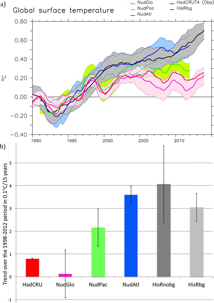
(a) Time evolution of the monthly mean global temperature centered over the period 1990–1994. In red is the HadCRUT4 observation-based dataset, in black is HisRbg ensemble, in blue the NudAtl, in green the NudPac, and in pink the NudGlo (cf. Table 1 for the name of the experiments). The error bars are computed as the spread of the five members of each ensemble around the ensemble mean. All simulation dataset has been masked to be comparable to observations (cf. experimental design). A 24-month running mean has been applied to all time series for readability. (b) Trend in global temperature over the period 1998–2012 in the HadCRUT4 observation and in the different simulations (Table 1). The error bar is computed from the five members considered in each ensemble of experiments. To compare correctly HadCRUT4 and the simulations, we apply the same spatial mask in the simulations from that available for the data, and we consider SST when over the ocean and 2-meter temperature when over the land as surface temperature, following what has been done in HadCRUT4 dataset. Masquer
(a) Time evolution of the monthly mean global temperature centered over the period 1990–1994. In red is the HadCRUT4 observation-based dataset, in black is HisRbg ensemble, in blue the NudAtl, in green the NudPac, and in pink the ... Lire la suite
The linear trend over the 1998–2012 period is extracted for each set of simulations and shown in Fig. 3b, together with the associated error bar. It confirms the visual inspection of Fig. 3a: only the trend in the NudGlo ensemble lies within the error bar of the observations, all the others show a larger warming over this period. The NudPac ensemble is nevertheless capturing a weaker trend than the others, especially when compared with the other partially nudged NudAtl simulations. These results suggest that in the IPSL–CM5A–LR model, the equatorial Pacific partly paces the global temperature (notably through global teleconnections), while it is not the case for the Atlantic. Furthermore, NudPac simulations still overestimate the observed trend by 0.1 °C/15 years. We find that the inclusion of the background volcanic forcing precisely induces such a reduction in the trend, as illustrated by the difference HisRbg minus HisRnobg. Thus, correct variations in the eastern tropical Pacific and volcanic forcing could be sufficient, under linear assumption, to correctly reproduce the hiatus in this model.
3.2 Spatial pattern of temperature trends for the period 1998–2012.
To go one step further, we compute the 15-year trend of the target period at each grid point and compare the spatial structure of the local trends of temperature in the observation and the different simulations (Fig. 4). We first check that the spatial average of these local trends equals the trend of the spatial average discussed in Fig. 3b, since non-linearity could question the usefulness of this diagnostic. The difference amounts to less than 5% of the global trend for all the simulations and HadCRUT4 data when using annual mean value. Thus, we argue that the map of local trends is a relevant diagnostic to explain the trend of the global temperature.

Spatial map of surface temperature trend (in 0.1 °C/yr) over the period 1998–2012. The significant trends following a two-sided student test are stippled in black. (a) HadCRUT4 data, (b) NudGlo ensemble mean, (c) NudPac ensemble mean, (d) NudAtl ensemble mean, (e) HisRnobg ensemble, and (f) HisRbg ensemble mean.
The HadCRUT4 pattern (Fig. 4a) shows that the observed hiatus is primarily related to the cooling of a large portion of the Pacific Ocean as well as a large cooling over Asia. In contrast, the two different sets of historical simulations, which show very similar patterns of temperature trends (Fig. 4e and f), exhibit a large warming of the Northern Hemisphere and tropical area. They show a small warming of the Southern Hemisphere, which is even experiencing a cooling in several areas of the mid-latitudes. Such a pattern is consistent with global warming (Stocker et al., 2013) or response to solar variations (Swingedouw et al., 2011). A recent study highlighted the role of the Deacon cell in this hemispheric adjustment (Armour et al., 2016). These results show that the observed cooling in the North Pacific is generally not driven by external forcing, except perhaps for the Northeast Pacific region, which shows a slight cooling trend in these simulations.
In NudGlo, the temperature pattern is generally similar to the observed one (Fig. 4b), with a cooling in the West Pacific both in tropical and high latitudes areas, a warming in the west high latitudes Pacific, a warming in the tropical Atlantic and a cooling in the central North Atlantic. This indicates that NudGlo succeeds in capturing the main feature of SST trends for the 1998–2012 period. NudPac shows no large-scale significant warming in the eastern tropical Pacific, in agreement with NudGlo and HadCRUT4, and contrarily to NudAtl and historical ensembles. In NudAtl, the general temperature trend pattern observed in the Atlantic, where nudging is applied, is reproduced, although the cooling area in the northern mid-latitudes is not entirely captured. This may be due to the strong internal variability in this region of deep mixed layer, which can overwhelm the nudging constraint (Ortega et al., 2017). The tropical Pacific is strongly warming as compared to NudPac. This response of the tropical Pacific may explain the large warming at the global scale observed in the NudAtl ensemble of simulations (Fig. 3b).
Thus, while the tropical Pacific succeeds in attenuating the global mean surface warming (NudPac), the Atlantic is not capable of driving the observed changes in the Pacific Ocean and NudAtl is therefore not reproducing the hiatus.
3.3 Dynamical response
The trends of sea-level pressure (SLP) and surface wind velocity (Fig. 5) in the 20CR reanalysis show a clear increase in the easterlies over most of the tropical Pacific Ocean for the period 1998–2012, associated with a positive SLP trend in the southeastern Pacific. In the Atlantic and Indian sector, the SLP is anomalously negative. An anomalous easterly trend is also detected in the Indian Ocean. We notice a pattern resembling a Rossby wave emanating from the tropical Pacific towards Antarctica and up to the southern Indian Ocean, with alternate positive and negative SLP poles. In the Northern Hemisphere, such a pattern in the trends is less clear, but we note a trend towards high pressure over the Aleutian low, and over Iceland, while trends over the Azores high is rather negative. This resembles a trend towards a negative phase of the Arctic Oscillation.

Spatial map of sea-level pressure trend (in dPa/yr) over the period 1998–2012 as well as trend in wind velocity as arrows. (a) NOAA-20CR reanalysis data, (b) NudGlo ensemble mean, (c) NudPac ensemble mean, (d) NudAtl ensemble mean, (e) HisRnobg ensemble, and (f) HisRbg ensemble mean. The green box in (a) corresponds to the average area in Fig. 6.
None of the two historical ensembles, which show once again very similar patterns at all latitudes, capture the amplitude of SLP and wind anomalies in the tropical Pacific. On the other hand, they reproduce the positive SLP trend of the Aleutian low, associated with the local cooling trend seen in Fig. 4 via advection of cold Arctic air in the central Pacific. This confirms that the external forcing (most probably anthropogenic aerosols, cf. Smith et al., 2016, Takahashi and Watanabe, 2016) may have played a role in these simulations as well as in the real system.
The signs of the SLP trends in the different tropical oceanic basins are captured in NudGlo. The teleconnection with the Aleutian low is relatively well-reproduced in the Northern Hemisphere, in contrast to the teleconnection pattern in the Southern Hemisphere, where few direct observations are available. The NudPac ensemble can reproduce the positive trend in the subtropical regions of the Pacific and the negative one in the Indian Ocean. The SLP trend over the tropical Atlantic basin is less well reproduced, as well as the wave patterns towards midlatitudes in both hemispheres. At high latitudes, the response is characterized by a negative trend over the North Pole and a positive trend over the South Pole, in a fashion similar to what is found in both historical sets, but differing from the observations. SST nudging in the North Atlantic (NudAtl) leads to a SLP trend of opposite sign in all basins, while the anomaly in the southern Ocean is again as in the historical simulations.
We also find an increase in the trade winds (easterlies) in the tropical West Pacific in most of the ensembles, except NudAtl. Focusing on the box analysed in England et al. (2014, cf. fig. 5), Fig. 6 confirms this increase in zonal wind speed. Nevertheless, the amplitude of the trend over the 1990s and the 2000s is more than four times weaker in the two historical ensembles as compared to observations. This is smaller than the ratio found by Takahashi and Watanabe (2016), who were suggesting that the anthropogenic aerosols account for about one third of the wind stress trend over the same time period, but of magnitude comparable to the results of England et al. (2014). The amplitude of the trend is also underestimated in NudGlo and NudPac by about a factor of two. This may indicate that the anomalous wind changes are only partially forced by the SST gradient and that unforced stochastic variations may play for about half (according to our simulations) of the observed wind trend in the tropical area. Alternatively, an underestimation of the SST-wind coupling in this model, or a too weak constrain applied on the SST as compared to Kosaka and Xie (2013), could be at the origin of the lack of zonal wind intensification in the equatorial Pacific in our nudged simulations.
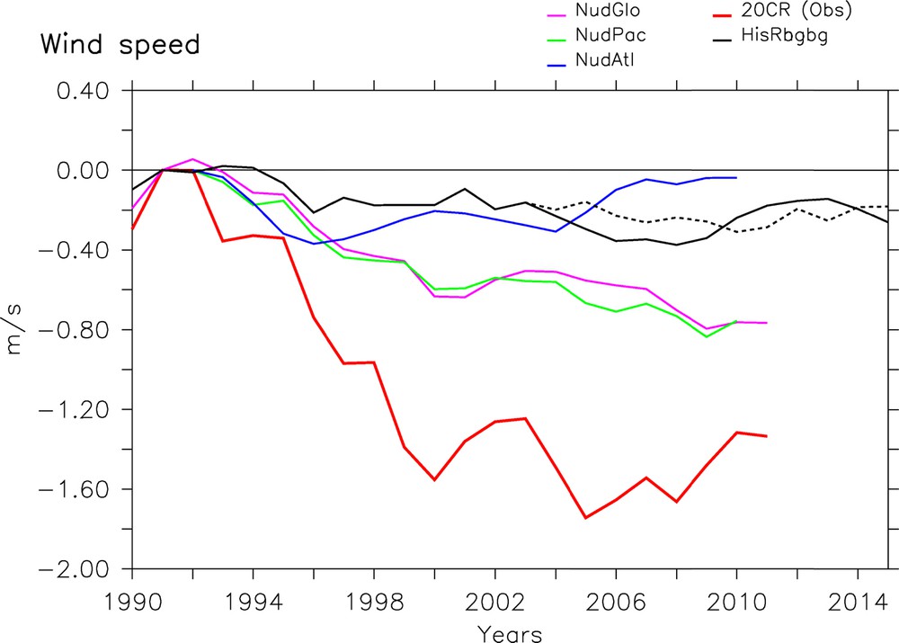
Wind velocity in the western tropical Pacific (6°S–6°N, 150°W–180°W, cf. Fig. 5a) in the different simulations, following the box definition from England et al. (2014). A 5-year running mean has been applied on all time series, and they have been centered over the mean of the years 1990–1994.
4 Discussions and conclusions
While the hiatus in global mean temperature has been analysed for different time periods in previous studies, we find here that the 1998–2012 one is the lowest 15-year trend of the last few decades, and that trends computed over 20 years show a weaker hiatus (not shown). We have therefore focused our analysis on this period. We have compared, using the IPSL–CM5A–LR model, historical simulations with different external forcing, accounting (HisRbg) or not (HisRnobg) for the effect of background volcanic eruptions from 2006, and globally (NudGlo) or partially (NudPac in the East tropical Pacific and NudAtl over the whole Atlantic) SST-nudged simulations to track the processes potentially explaining this hiatus period.
We find that historical simulations without background volcanoes overestimate the observed trend in global temperature by a factor of 4, and only of 3 if background volcanoes are incorporated from 2006 onward. Nudging over the whole ocean is sufficient to reproduce the hiatus, which is reasonable given that the ocean covers 70% of the Earth. SST nudging only imposed over the eastern Pacific (8% of the Earth) is increasing the agreement with observations (dividing the trend of HisRbg by a factor of two), so that accounting both for variability in the East tropical Pacific and including background volcanoes of similar amplitude as that observed, can succeed, under linear assumption, in reproducing the hiatus trend. On the contrary, NudAtl is similar to HisRnobg, so that nudging the Atlantic basin (15% of the Earth) has no effect on the global average representation of the hiatus in the IPSL–CM5A–LR model. In this respect, nudging over an almost twice-smaller region (NudPac as compared to NudAtl) can have very different effects on the global temperature, illustrating the complexity of the dynamics of the Earth system.
It is striking in our simulations that the Pacific adjustment in NudAtl is opposed to the one imposed in NudGlo and NudPac. The Atlantic adjustment in NudPac is also very different from the one imposed in NudAtl. One could thus suspect a biased link between the Atlantic and the Pacific in the model. The link between Atlantic and Pacific main modes of variability (AMV–Atlantic Multidecadal Oscillation–and PDO) has been analysed by Marini and Frankignoul (2014) in the observed data set. They find a significant link where a positive AMV leads by one decade a negative PDO, although this link is at the limit of statistical significance due to the short instrumental time frame. In the IPSL-CM5A-LR model, we found in the 1000-year long pre-industrial simulation a maximum correlation in phase, with a positive AMV associated with a positive PDO (not shown). This may confirm that the mechanisms relating the two basins are not well represented in this particular model, under the assumption that the observed signal is significant. In this context, we cannot conclude on the possible teleconnections between the Atlantic and the Pacific basin at play during the hiatus period.
The link between the Atlantic and the Pacific can also be modulated by the state of the Indian Ocean. Indeed, Terray et al. (2016) and Kajtar et al. (2016) showed on a shorter time frame that the influence of the Atlantic Ocean on the El Niño Southern Oscillation (ENSO) dynamics is largely dependent on the Indian Ocean state as well. Since the PDO is related with the low-frequency variations of ENSO (Newman et al., 2016), the state of the Indian Ocean may also have played a role during the hiatus period (e.g., Luo et al., 2012; Mochizuki et al., 2016). An interesting additional pacemaker experiment would thus be to drive the Indian Ocean as well, or the tropical Indian, Atlantic and Pacific oceans together, to explore if the influence on the tropical Pacific is clearer when tropical Atlantic and Indian oceans are both also constrained.
Another possibility to explain the lack of hiatus in NudAtl is the adjustment of the IPSL–CM5A–LR climate model to zonal SST gradients between the different tropical basins. The dynamics induced by the Atlantic–Pacific gradient over the last three decades has been nicely illustrated in Li et al. (2016). They showed that in simulations of the CESM–CAM climate model, a large warming in the Atlantic sector firstly induces a change in wind velocity over the tropical area through the so-called Gill (1980) response (see fig. 3 from Li et al., 2016). Indeed, as shown in Gill (1980), a diabatic heating anomaly located in the Atlantic is inducing the emission of Kelvin waves east of the anomaly, which weaken the westward wind velocity over the equatorial Indian Ocean and slightly enhance the easterlies over the western Pacific. Through changes in latent heat fluxes, this tends to warm the Indian Ocean and slightly cool the western Pacific. West of the diabatic heating, two Rossby wave packets are emitted on each side of the equator (cf. Gill, 1980). These waves tend to increase the off-equatorial westerlies and decrease the equatorial easterlies (cf. fig. 1 of Gill, 1980, and fig. 2a of Li et al., 2016). At the equator, the decrease in upwelling and latent heat flux should increase the surface temperature, while off the equator the increase in latent heat flux should lead to cooling.
Therefore, in a first phase, the response to diabatic heating in the Atlantic is complex and leads to warming in the East equatorial Pacific and cooling in the West Pacific, which would tend to activate a Niño-like response (e.g., Lengaigne et al., 2004). Nevertheless, the warming of the Indian and the cooling off equatorial East Pacific, when they propagate to West Pacific and East Pacific, respectively, should, on the opposite, favour a Niña-like response. This is the subtle interplay between these two opposing signatures that will activate in a second phase the Bjerknes feedback into one direction (Niña-like) or the other (Niño-like). While Li et al. (2016) argued that the interplay between these two effects would mostly favour a Niña-like signature, it is possible that a slight difference in the impact of the diabatic heating from the Atlantic could as well activate a Niño-like response. This seems to be what happened in our NudAtl ensemble. Consequently, the response to diabatic heating in the Atlantic may not be so straightforward, and slight differences in the background states (for instance from the Indian Ocean) can lead a response opposite to the one shown in Li et al. (2016).
The poor performance in terms of hiatus reproduction of NudAtl is thus due to an opposite link between Atlantic and Pacific Oceans as compared to the one suggested in other studies (Mcgregor et al., 2014; Takahashi and Watanabe, 2016) or in observations (Marini and Frankignoul, 2014). This shows that this supposed link is not captured in this model. Nevertheless, we insist here that the observed link between decadal variation of the AMV and PDO (Marini and Frankignoul, 2014) was found on a very short record for observations (around one century), which questions the statistical significance of this result as stated by Marini and Frankignoul (2014). Analysing the Atlantic–Pacific connections on a longer time frame than the last century will be necessary to better assess the existence of the Atlantic-Pacific link in the real system. A better characterisation of the processes at play during the hiatus, and the possible link between Pacific and Atlantic basins, will strongly benefit from on-going CMIP6 intercomparison project dedicated to pacemaker experiments (Boer et al., 2016), where either the Atlantic or the Pacific will be nudged towards observations (dcppC–pac–pacemaker and dcppC–atl–pacemaker–see Boer et al., 2016). Furthermore, the potential role played by the Indian Ocean for the hiatus period remains to be evaluated.
Acknowledgments
This research was partly funded by the ANR MORDICUS project (ANR-13-SENV-0002-02). It is also funded by the SPECS project funded by the European Commission's Seventh Framework Research Programme under the grant agreement No. 308378. This work was granted access to the HPC resources of TGCC under the allocation No. 2016-017403. We thank Patrick Brockmann for help with figure design. This paper was solicited by the Chief Editor as part of a series of invited papers from laureates of the 2015 prizes of the French Academy of Sciences.