Simulation of seismic-prospecting random noise in the desert by a Brownian-motion-based parametric modeling algorithm

Tie Zhong; Shuo Zhang; Yue Li; Baojun Yang

doi:10.1016/j.crte.2018.07.003

Internal Geophysics (Seismology)

Simulation of seismic-prospecting random noise in the desert by a Brownian-motion-based parametric modeling algorithm

Présenté par : Handled by Michel Campillo

Tie Zhong ¹ ; Shuo Zhang ¹ ; Yue Li ² ; Baojun Yang ³

¹ Northeast Electric Power University, Department of Communication Engineering, Jilin, China
² Jilin University, Department of Information Engineering, 130012 Jilin, China
³ Jilin University, Department of Geophysics, Jilin, China

Comptes Rendus. Géoscience, Volume 351 (2019) no. 1, pp. 10-16.

Résumé

Random noise has a negative impact on seismic-prospecting record processing. An important step to improve the methods aimed at the attenuation of random noise is to scientifically characterize the properties of the noise. Numerical modeling is useful to understand the nature of the random noise. In this study, we present a Brownian-motion-based parametric modeling algorithm for the simulation of seismic-prospecting random noise in the desert. The optimal Hurst exponent required to implement the method can be determined by comparing the spectral properties related to the noise data and the simulated results. The data used to analyze the properties of the noise were acquired in the Tarim Basin (Northwest of China). We verify the performance of the modeling algorithm by comparing the results obtained after the simulation with the real noise data in both the time domain and the spatio-temporal domain. The experimental results thus obtained prove the accuracy and efficiency of the proposed modeling algorithm. This study can be used as a basis to investigate the seismic-prospecting random noise characteristics and thus contribute to its mitigation.

Métadonnées

Reçu le : 2018-07-08
Accepté le : 2018-07-09
Publié le : 2018-08-08

DOI : 10.1016/j.crte.2018.07.003

Mots clés : Seismic prospecting, Random noise, Fractional Brownian Motion, Parametric modeling algorithm

Affiliations des auteurs :

Tie Zhong ¹ ; Shuo Zhang ¹ ; Yue Li ² ; Baojun Yang ³

¹ Northeast Electric Power University, Department of Communication Engineering, Jilin, China
² Jilin University, Department of Information Engineering, 130012 Jilin, China
³ Jilin University, Department of Geophysics, Jilin, China

@article{CRGEOS_2019__351_1_10_0,
     author = {Tie Zhong and Shuo Zhang and Yue Li and Baojun Yang},
     title = {Simulation of seismic-prospecting random noise in the desert by a {Brownian-motion-based} parametric modeling algorithm},
     journal = {Comptes Rendus. G\'eoscience},
     pages = {10--16},
     publisher = {Elsevier},
     volume = {351},
     number = {1},
     year = {2019},
     doi = {10.1016/j.crte.2018.07.003},
     language = {en},
}

TY  - JOUR
AU  - Tie Zhong
AU  - Shuo Zhang
AU  - Yue Li
AU  - Baojun Yang
TI  - Simulation of seismic-prospecting random noise in the desert by a Brownian-motion-based parametric modeling algorithm
JO  - Comptes Rendus. Géoscience
PY  - 2019
SP  - 10
EP  - 16
VL  - 351
IS  - 1
PB  - Elsevier
DO  - 10.1016/j.crte.2018.07.003
LA  - en
ID  - CRGEOS_2019__351_1_10_0
ER  -

%0 Journal Article
%A Tie Zhong
%A Shuo Zhang
%A Yue Li
%A Baojun Yang
%T Simulation of seismic-prospecting random noise in the desert by a Brownian-motion-based parametric modeling algorithm
%J Comptes Rendus. Géoscience
%D 2019
%P 10-16
%V 351
%N 1
%I Elsevier
%R 10.1016/j.crte.2018.07.003
%G en
%F CRGEOS_2019__351_1_10_0

Tie Zhong; Shuo Zhang; Yue Li; Baojun Yang. Simulation of seismic-prospecting random noise in the desert by a Brownian-motion-based parametric modeling algorithm. Comptes Rendus. Géoscience, Volume 351 (2019) no. 1, pp. 10-16. doi : 10.1016/j.crte.2018.07.003. https://comptes-rendus.academie-sciences.fr/geoscience/articles/10.1016/j.crte.2018.07.003/

Version originale du texte intégral

1 Introduction

Seismic prospecting is the most widely used method for oil–gas and mineral exploration. With the depletion of the easy-explored resources, exploration must be carried out in deep reservoirs and irregular layers, which presents significant challenges (Wu et al., 2016). High-quality seismic records can help to achieve high-accuracy seismic prospecting, especially in complex strata (Li et al., 2017). Random noise is the key factor that impacts the signal-to-noise ratio (SNR) of seismic records; further, its irregular interference complicates seismic data processing. Here, random noise refers to the incoherent noise in seismic records, which primarily originates from wind motion, environmental noise, noise from recording instruments, and geophones loosely coupled with the ground (Yilmaz, 2001). Understanding the properties of random noise is the prerequisite for designing noise mitigation methods (Xiong et al., 2014; Zhong et al., 2015; Zhuang et al., 2015). Recently, the properties of the random seismic noise have attracted increasing attention in geophysics, and several important results have been obtained (Akhouayri et al., 2011; Groos and Ritter, 2009; Groos et al., 2012). However, most of these studies focused on the statistical properties of the seismic noise, which can only provide a qualitative judgment of the random noise, such as whether seismic noise is stationary. Obtaining quantitative results of the random noise by investigating the random noise modeling problem is of more practical importance (Li and Li, 2015b; Zhong et al., 2016; Zhong et al., 2017). Hence, we herein focus on the parametric modeling algorithm for seismic-prospecting random noise.

Modeling research is useful to understand the nature and analyze seismic noise generation mechanisms. Recently, the properties of seismic noise resources have been extensively discussed, and the findings can be used as the theoretical foundation for the modeling algorithm. In noise modeling, the use of wave equation theory to simulate seismic noise has yielded a significant advance in recent years (Li and Li, 2015a; Li et al., 2017). According to the random noise characteristics, the functions of different noise sources, which propagate by the wave equation, can be determined. Hence, random noise can be viewed as a superimposed wave field excited by several independent sources in a homogeneous isotropic half-space. Similarly, the modeling algorithm for random seismic noise in a desert area is investigated (Li and Li, 2015a), and the influences of environmental conditions, such as wind speed and surface roughness, are also discussed.

However, the wave-equation-based modeling algorithm is complex and the findings cannot be directly applied to noise attenuation. Therefore, research on statistical parametric modeling algorithms for random seismic noise, which aims at revealing the underlying stochastic processes, appears to have more practical significance. Specifically, if a known stochastic process can be used to represent the seismic noise, the process findings can be introduced in seismic noise attenuation. Random-noise modeling from a stochastic perspective is first proposed in seismic noise-field analysis. When processing the seismic records collected at seismological stations, Caserta et al. (2007) proposed that seismic noise has a super-diffuse nature, which means that noise has a persistent Markovian character with a memory longer than ordinary Brownian motion. Similarly, Mulargia (2012) and Pilz and Parolai (2014) also proposed that the seismic noise wave field is not diffuse. Owing to the differences in the frequency bands concerned, these findings cannot be directly used to represent the seismic-prospecting random noise. However, all these studies indicate that random noise is related to fractional Brownian motion (FBM) (Mandelbrot and Ness, 1968). Recently, some studies have shown that seismic noise is similar to FBM series in power spectral density (PSD), whose energy are primarily concentrated in the low-frequency bands (Li and Li, 2015a; Mandjes, 2008; Zhong et al., 2015). Based on these findings, it is feasible to simulate the seismic-prospecting random noise using the FBM theory.

The rest of this paper is organized as follows: the theoretical background of the proposed modeling algorithm is introduced in Section 2, which includes the descriptions for the FBM theory and the principle for the modeling methodology; Section 3 mentions real noise data and acquisition conditions; Section 4 presents the numerical experiments performed to verify the efficiency of the proposed methodology using both time-domain analysis and spatio-temporal analysis; finally, we present our conclusions in Section 5.

2 Theory

In this section, we briefly describe the principle and properties of the FBM theory, which is used as the basis of the modeling algorithm. Then we explain in detail the methodology developed.

2.1 Fractional Brownian motion

The FBM is one of the most commonly used stochastic processes. According to probability theory, a generalized Brownian motion can be viewed as a continuous Gaussian process over time. Generally, the FBM is a moving average in which the past increments are weighted by kernel functions. Mandelbrot and Ness (1968) presented a precise expression for the FBM, which is denoted as B_H(t):

B_{H} (t) - B_{H} (0) = \frac{1}{Γ (H + 1 / 2)} \{\int_{- \infty}^{0} [{(t - s)}^{H - 1 / 2} - {(- s)}^{H - 1 / 2}] d B (s) + \int_{0}^{t} {(t - s)}^{H - 1 / 2} d B (s)\}

(1)

where B(t), which is equal to B_1/2(t), denotes an ordinary Brownian motion; B_H(0) is a known value; Γ(H + 1/2) is a gamma function. The H parameter, called the Hurst exponent, is used as a measure of the long-term memory of a time series. This exponent varies from 0 to 1 and describes the irregularity of the resultant motion; the higher the value of H, the smoother the motion. Thus, the FBM series with different properties can be obtained by modifying the Hurst exponent.

The FBM has several important characteristics, namely:

(a) the increment B_H(t)–B_H(t–1) is stationary and follows a Gaussian distribution,

B_{H} (t + 1) - B_{H} (t) \sim N (0, σ^{2}),

(2)

(b) the FBM process is the only self-similar Gaussian process,

B_{H} (a t) \sim {|a|}^{H} B_{H} (t)

(3)

E [{|B_{H} (t + 1) - B_{H} (t)|}^{2}] \propto \frac{1}{{|τ|}^{2 H}} E [{|B_{H} (t + τ) - B_{H} (t)|}^{2}],

(4)

(c) the mean square of the increment is directly proportional to the changing time range,

E [{|B_{H} (t + τ) - B_{H} (t)|}^{2}] \propto {|τ|}^{2 H} .

(5)

Several effective algorithms have been proposed for the FBM series generation, such as the wavelet-based synthesis algorithm (Abry and Sellan, 2008), successive random additions methods (Mcgaughey and Aitken, 2000), and the random midpoint displacement (RMD) algorithm (Norros et al., 2000). The RMD algorithm has a relatively low computation cost and can provide an accurate simulation series. Therefore, in this study, we used the RMD algorithm to generate the FBM series. The basic principle of the RMD algorithm is based on bisections and interpolations. Owing to the self-similarity of the FBM process, the midpoint and endpoint values for a given interval can be randomly selected according to the corresponding distributions. Therefore, the realization of an FBM process could be obtained iteratively. More details about this process can be found in Norros et al. (2000).

2.2 Modeling algorithm

An FBM series always has a color spectrum, and the PSD can be approximately denoted as f^1–2H, where f represents the frequency and H is the Hurst exponent. Similarly, the seismic-prospecting random noise is also a type of “1/f noise,” whose energy is primarily concentrated in the low-frequency band. Fig. 1 shows the comparison between a field noise series in desert and an FBM series with a Hurst exponent of 0.9. As shown in this figure through the respective PSD functions, the FBM series and the noise data have a similar energy distribution, especially in the middle-frequency range [50–400 Hz]. Therefore, using the FBM to model the random seismic noise in desert is reasonable.

Fig. 1
Waveform (up) and normalized PSD (down) of an FBM series (a). Waveform and normalized PSD of a noise series (b).

Here, the multitaper method (Thomson, 2005), which is a popular signal processing algorithm, is used to estimate the PSD of the series. This method overcomes some of the limitations of the conventional Fourier analysis, especially in terms of spectrum leakage, estimation error, and frequency resolution. In general, the result of the PSD estimation for a given series x(n) can be denoted as

S (f) = \frac{1}{K} \sum_{k = 1}^{K} {|\sum_{n = 0}^{N - 1} d_{k} (n) x (n) \exp (- j 2 π f n)|}^{2}

(6)

where d_k(n), which is selected from the discrete prolate spheroidal sequences, denotes the window functions.

In practice, the amplitude response of the geophone used and the truncation effect of the recording instrument affect the seismic record. To demonstrate the effects of the geophones and recording instruments in detail, we calculated the normalized PSD of a field noise series, and the results are shown in Fig. 2. As can be seen, the attenuation effects for the components below 10 Hz or above 400 Hz are conspicuous, so that these effects should be considered as band-pass filtering in the modeling process.

Fig. 2
Effects of the instrumentation on the normalized PSD of a noise series. Left bottom corner: enlarged view of the beginning of the noise signal bounded by a rectangle.

Therefore, in this study we follow FBM theory to simulate background seismic noise and use a band-pass filter to represent the effects of the recording systems. Hence, the random noise modeling algorithm can be generalized as

y (n) = \sum_{l = - \infty}^{\infty} B_{H} (l) h (n - l)

(7)

where y(n) denotes the result of the noise simulation, and B_H(l) is an FBM series with a known Hurst exponent (H). Moreover, h(n) represents a band-pass filter with corner frequencies of 10 Hz and 400 Hz. In Eq. (7), the Hurst exponent is used to amend the irregularity of the simulation outputs. The optimal Hurst exponent value is determined by comparing the simulation results to the real noise data in terms of PSD. Generally, the optimal value of the parameter H is the solution of the following optimization problem:

\begin{array}{l} \min_{H} E [(\frac{1}{K} \sum_{k = 1}^{K} {|\sum_{n = 0}^{N - 1} d_{k} (n) x (n) e^{- j 2 π f n}|}^{2} - \frac{1}{K} \sum_{k = 1}^{K} {|\sum_{n = 0}^{N - 1} d_{k} (n) \sum_{l = - \infty}^{\infty} B_{H} (l) h (n - 1) e^{- j 2 π f n}|}^{2})] \\ s u b j e c t t o \sum_{f = 0}^{M - 1} \sum_{k = 1}^{K} {|\sum_{n = 0}^{N - 1} d_{k} (n) x (n) e^{- j 2 π f n}|}^{2} = \sum_{f = 0}^{M - 1} \sum_{k = 1}^{K} {|\sum_{n = 0}^{N - 1} d_{k} (n) \sum_{l = - \infty}^{\infty} B_{H} (l) h (n - 1) e^{- j 2 π f n}|}^{2} \end{array}

(8)

From these equations, we can conclude that the optimal result of the simulation has the most similar PSD with respect to the noise data analyzed. In summary, once the optimal value H_opt of the Hurst exponent is determined, the synthetic noise can be formulated as follows:

y_{opt} (n) = \sum_{l = - \infty}^{\infty} B_{H_{opt}} (l) h (n - 1)

(9)

3 Real noise data

The dataset for analysis comprises passive noise records collected by a receiver array deployed in the Tarim Basin in West China. This basin is mostly flat with no vegetation. The random noise is considered to be driven primarily by wind friction over the ground surface. The experimental seismic array, which meets the requirements generally adopted in seismic prospecting, consists of 512 geophones arranged in a single survey line at intervals of 50 m. The sampling interval is 1 ms. The geophone used is the JF-20DX-10, whose amplitude response is similar to a high-pass filter with a corner frequency of 10 Hz.

As is well known, whereas no shooting is being done, the sources of coherent noise in land-seismic prospecting come mainly from vehicle traffic, machinery, and 60-Hz (or 50-Hz) power lines (Cooper and Cook, 1984). Since our acquisitions are performed in remote areas, the cultural noise is relatively low. As an example, Fig. 3 shows a 5-s noise record acquired in the Tarim Basin, in which no obvious coherent noise can be observed in the record.

Fig. 3
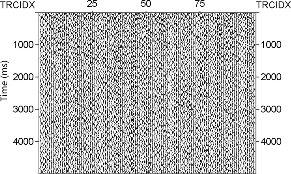
Field random noise data recorded in a desert area. (The number of traces is 100 and the recording time is 5 s.).

4 Results

We applied the proposed modeling algorithm to simulate seismic-prospecting random noise. To verify the performance of the modeling method, the waveforms of the real noise and synthetic noise data and their respective properties are compared in the time domain and the spatio-temporal domain. In general, these properties are investigated through the spectral characteristics, the statistical characteristics, and the phase space.

4.1 Checking results in the time domain

Here, we perform a detailed comparison between the real noise data and synthetic noise records in the time domain, such as the PSD and phase space. Fig. 4a shows the waveforms for a real noise series (top) and a synthetic noise record with a Hurst exponent of 0.95 (bottom). This figure shows that the real noise data and the synthetic noise series have almost the same fluctuation tendency and a strong resemblance. Fig. 4b shows the respective PSD functions of both noise series that reveal similar spectral characteristics. Both real noise and simulated noise keep a great resemblance, with the energy concentrated in the [0–30 Hz] frequency band. All these results support the efficiency of the proposed modeling method.

Fig. 4
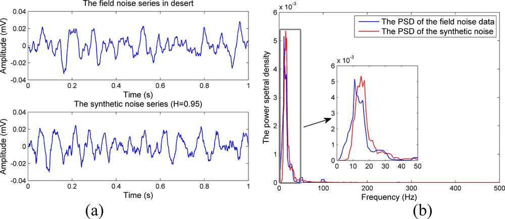
Comparison between real (up) and synthetic noise (down) waveforms (a). Respective PSD functions of both noise series (b). In the middle: enlarged view of the beginning of the PSD functions.

Fig. 5 allows the analysis of the statistical properties of the real noise data and the synthetic noise series. In this illustration, we compare the results obtained from the noise data by means of the amplitude distributions and cumulative distribution functions. The plots in Fig. 5a present the probability distributions of the real noise and synthetic record, respectively. The comparison results reveal that the histograms of the corresponding noise data are similar in trend, and the amplitudes centralize at approximately [–0.02, 0.02]. Moreover, the cumulative distribution curves presented in Fig. 5b are almost the same, except a slight difference appearing in the interval [0.005, 0.015]. In summary, the field and synthetic noise records have similar statistical characteristics.

Fig. 5
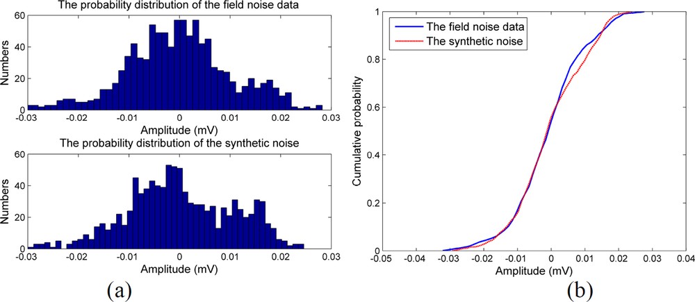
Histograms of amplitude distributions for real (up) and synthetic noise (down) (a); cumulative distribution curves for field noise and synthetic noise (b).

The chaotic properties attributed to random seismic noise (Wang et al., 2016) also serve to verify the efficiency of the modeling algorithm. In Fig. 6 we have drawn the orbits in the phase space corresponding to the series of field noise (Fig. 6a) and synthetic noise (Fig. 6b). These orbits, as may well be appreciated, are very similar. From the previous experiments, we conclude that the field noise data and the synthetic noise records have similar characteristics, and that the modeling algorithm is feasible.

Fig. 6
View of the chaotic nature of the ambient seismic noise: a: orbits in the phase space related to the series of field noise; b: orbit in the phase space related to the synthetic noise series.

4.2 Checking results in the spatio–temporal domain

For further verifying the efficiency of the simulation algorithm, we selected a noise record acquired in the desert to obtain the simulation results when applying the proposed method. In Fig. 7, we show a real noise record composed of 50 traces up to a time of 1 s, collected in the course of a seismic survey in the Tarim Basin, and right next to it we show the synthetic noise record. As before, one can see that the two records have similar vibration patterns.

Fig. 7
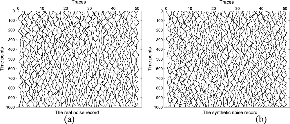
Real noise record (a) versus synthetic noise record (b). (The noise data were acquired in the Tarim Basin. In both cases the number of traces is 50 up to a time of 1 s.).

While the seismic noise data can be seen as a 2-D dataset, the properties of the random seismic noise change both in the time direction and the spatio–temporal domain. The noise characteristics, when analyzed using a 2-D Fourier transform, can also be explored through the signature of the f–k spectrum after converting the noise data in the spatio–temporal domain to the frequency–wavenumber domain. Fig. 8 shows the f–k spectra of the real and simulated noise data records. Again we find that these two f–k spectra for real and synthetic noise are quite similar.

Fig. 8
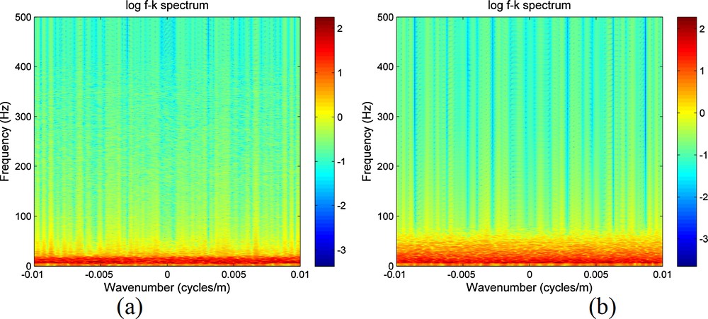
Frequency-wavenumber diagram (f–k spectrum) of the real (a) and simulated (b) noise data records.

In addition to qualitative comparisons, a quantitative analysis is perhaps more informative to the extent that it provides more precisely the characteristics of the noise data. It is known that statistical properties can be expressed by statistical moments. In this sense, we calculated several high-order moments, such as the mean, variance, kurtosis, and skewness, which facilitate the presentation of data properties at a certain level. The comparison of statistical moments for real noise data and synthetic noise data is shown in Table 1. We see that the differences between these statistical moments are relatively small; in particular, the variance is almost the same, while the other moments take slightly smaller values for synthetic noise than for real noise. The results concerning kurtosis and skewness indicate that both the real noise and the synthetic data have symmetric character that is close to a Gaussian distribution. Given the similarity of the spatio-temporal characteristics of the real and synthetic noise data, the efficiency and accuracy of the Brownian-motion-based noise-modeling algorithm seems to be guaranteed.

Table 1

	Mean	Variance	Kurtosis	Skewness
Real noise	–3.67 × 10⁻⁴	8.12 × 10⁻⁴	3.154	0.07
Synthetic noise	–2.02 × 10⁻⁴	8.13 × 10⁻⁴	2.929	–0.06

5 Conclusions

In this study, we investigate the seismic-prospecting random noise-modeling problem from a statistical viewpoint, by analyzing the stochastic process underlying the random noise. We follow the FBM theory to simulate background seismic noise, and we use a band-pass filter to control the effects of recording systems. The optimal Hurst exponent value is determined by comparing the simulation results to the real noise data in terms of PSD. The parametric modeling algorithm of random seismic noise that we propose is based on the similarity between the PSD of the real noise and the FBM process. We verify the performance of the processing scheme by comparing the simulated noise with the real noise data in both the time domain and the spatio-temporal domain. First, we focus our attention on the analysis of the statistical properties of real and simulated noise, as PSD, amplitude distribution, cumulative distribution curve, and behavior in the phase space. Second, we explore the noise characteristics through the frequency–wavenumber spectrum. The results reveal the similarity that the synthetic noise records keep with the real noise dataset. Hence, the noise generation algorithm, which uses the FBM theory to perform the modeling task, is feasible. In other words: the seismic-prospecting random noise can be considered as the production of a stochastic FBM process. The findings of this study are useful to develop better models for land-seismic-prospecting random noise, and also for noise reduction and signal-detection algorithms.

Acknowledgments

This research is financially supported by the National Natural Science Foundation of China (41730422), Postdoctoral Projects of the Science Foundation of China (2018M631839), the Foundation for Youth Excellence of the Jilin Scientific Committee (20180520091JH), and a Research Project of Jilin Province Education Department (JJKH20180420KJ).

Bibliographie

[Abry and Sellan, 2008] P. Abry; F. Sellan The Wavelet-Based Synthesis for Fractional Brownian Motion Proposed by F. Sellan and Y. Meyer: Remarks and Fast Implementation, Appl. Comput. Harmonic Anal., Volume 3 (2008) no. 4, pp. 377-383

[Akhouayri et al., 2011] E.S. Akhouayri; E. Hassan; A. Laasri et al. Signal stationarity testing and detecting of its abrupt change, Riyadh, Saudi Arabia (2011), pp. 1-5

[Caserta et al., 2007] A. Caserta; G. Consolini; P.D. Michelis Statistical features of the seismic noise-field, Studia Geophysica et Geodaetica, Volume 51 (2007) no. 2, pp. 255-266

[Cooper and Cook, 1984] H.W. Cooper; R.E. Cook Seismic data gathering, Proc. IEEE, Volume 72 (1984) no. 10, pp. 1266-1275

[Groos and Ritter, 2009] J.C. Groos; J.R.R. Ritter Time domain classification and quantification of seismic noise in an urban environment, Geophys. J. Int., Volume 179 (2009) no. 2, pp. 1213-1231

[Groos et al., 2012] J.C. Groos; S. Bussat; J.R.R. Ritter Performance of different processing schemes in seismic noise cross-correlations, Geophys. J. Int., Volume 188 (2012) no. 2, pp. 498-512

[Li and Li, 2015a] G. Li; Y. Li Random noise of seismic exploration in desert modeling and its applying in noise attenuation, Chin. J. Geophys., Volume 59 (2015) no. 2, pp. 683-692

[Li and Li, 2015b] G. Li; Y. Li Wave equation modeling of random noise in seismic exploration for metal deposits in mountainous areas, Chin. J. Geophys., Volume 59 (2015) no. 12, pp. 4577-4593

[Li et al., 2017] G. Li; Y. Li; B. Yang Seismic Exploration Random Noise on Land: Modeling and Application to Noise Suppression, IEEE Trans. Geosci. Remote Sensing, Volume PP (2017) no. 99, pp. 1-14

[Mandelbrot and Ness, 1968] B.B. Mandelbrot; J.W.V. Ness Fractional Brownian Motions, Fractional Noises and Applications, Siam Rev., Volume 10 (1968) no. 4, pp. 422-437

[Mandjes, 2008] M. Mandjes On spectral simulation of Fractional Brownian Motion, Probability Eng. Info. Sci., Volume 17 (2008) no. 3, pp. 177-191

[Mcgaughey and Aitken, 2000] D.R. Mcgaughey; G.J.M. Aitken Statistical analysis of successive random additions for generating fractional Brownian motion, Phys. A Stat. Mech. Appl., Volume 277 (2000) no. 1, pp. 25-34

[Mulargia, 2012] F. Mulargia The seismic noise wavefield is not diffuse, J. Acoust. Soc. Am., Volume 131 (2012) no. 4, p. 2853

[Norros et al., 2000] I. Norros; P. Mannersalo; J.L. Wang Simulation of Fractional Brownian Motion with Conditionalized Random Midpoint Displacement, Adv. Perform. Anal., Volume 17 (2000) no. 3, pp. 417-434

[Pilz and Parolai, 2014] M. Pilz; S. Parolai Statistical properties of the seismic noise field: influence of soil heterogeneities, Geophys. J. Int., Volume 199 (2014) no. 1, pp. 430-440

[Thomson, 2005] D.J. Thomson Spectrum estimation and harmonic analysis, Proc. IEEE, Volume 70 (2005) no. 9, pp. 1055-1096

[Wang et al., 2016] F. Wang; D. He; Y. Li Modeling Study of Chaotic Ambient Noise in Land Seismic Exploration, J. Jilin Univ. Info. Sci. Ed., Volume 34 (2016) no. 3, pp. 320-326

[Wu et al., 2016] N. Wu; Y. Li; Y. Tian et al. Trace-transform-based time-frequency filtering for seismic signal enhancement in Northeast China, C. R. Geosci., Volume 348 (2016), pp. 360-367

[Xiong et al., 2014] M. Xiong; Y. Li; N. Wu Random-Noise Attenuation for Seismic Data by Local Parallel Radial-Trace TFPF, IEEE Trans. Geosci. Remote Sensing, Volume 52 (2014) no. 7, pp. 4025-4031

[Yilmaz, 2001] O. Yilmaz Seismic Data Analysis: Processing, Inversion, and Interpretation of Seismic Data, Society of Exploration Geophysicists, Tulsa, OK, 2001 (169 p.)

[Zhong et al., 2015] T. Zhong; Y. Li; N. Wu et al. A study on the stationarity and Gaussianity of the background noise in land-seismic prospecting, Geophysics, Volume 80 (2015) no. 4, p. V67-V82

[Zhong et al., 2017] T. Zhong; Y. Li; B. Yang et al. Statistical features of the random noise in land seismic prospecting, Chin. J. Geophys., Volume 60 (2017) no. 2, pp. 654-664

[Zhong et al., 2016] T. Zhong; R.J. Song; Y. Li et al. A Study of the Parametric Modeling Algorithm for the Seismic Prospecting Random Noise, Conference on Geophysics for Mineral Exploration & Mining, 2016, pp. 1-5

[Zhuang et al., 2015] G. Zhuang; Y. Li; N. Wu et al. Curvature-Varying Hyperbolic Trace TFPF for Seismic Random Noise Attenuation, IEEE Geosci. Remote Sensing Lett., Volume 12 (2015) no. 11, pp. 2252-2256

Commentaires - Politique