

1 Introduction
Geological models honoring subsurface data are central objects involved in a wide spectrum of applications (Ringrose and Bentley, 2015). A model, whether it be three dimensional or two dimensional, is generally dedicated to answer one question at a given scale, e.g., contaminant transport (e.g., Huysmans and Dassargues, 2009), the impact of subsurface structures on ground motion (e.g., Benites and Olsen, 2005; Chaljub et al., 2010), the geomechanical behavior of a reservoir (e.g., Segura et al., 2011; Verdon et al., 2013). In most cases, the choice of this scale and of the adapted spatial resolution is complicated because very small geological features can have an important impact on the physical process. For instance, thin shale drapes in alluvial deposits may have a large impact on fluid circulations (e.g., Issautier et al., 2013; Jackson et al., 2000, 2009; Massart et al., 2016).
To simulate the physical processes in natural geological settings, most methods rely on a spatial discretization of the model, using a mesh or a grid (we use the term mesh for an unstructured spatial discretization). The mesh represents the model at a given level of detail and is used to simulate a given physical process. It should therefore capture all the geological features having a significant impact on that physical process and meet the requirements of the PDE discretization method in terms of mesh quality. These two objectives may often be conflicting because geometrical complexity is inherent in geological models (thin layers, stratigraphic unconformities, small fault displacements) (Graf and Therrien, 2008; Karimi-Fard and Durlofsky, 2016; Merland et al., 2014; Mustapha and Dimitrakopoulos, 2011; Pellerin et al., 2015). One solution is to solve the differential equations on a mesh that does not necessarily accounts for all geological discontinuities, e.g., using the extended finite-element method (XFEM) (Moës et al., 1999). Other options are to decrease the expected mesh quality criteria, or to first simplify the geometry of the input model.
In practice, most models are manually modified by skilled practitioners who are able to ensure that the generated mesh will fulfill the project requirements. A few automatic strategies exist to simplify the model before generating its mesh, but none ensures either the validity of the output model or its geological consistency (Karimi-Fard and Durlofsky, 2016; Mustapha and Dimitrakopoulos, 2011; Pellerin et al., 2014).
Another practical challenge also arises, since geomodeling methods do not always generate a sealed boundary representation. In this case, repairing (or sealing) is required to prepare the model for meshing. This repair process (e.g., Barequet and Kumar, 1997; Elsheikh and Elsheikh, 2012; Euler et al., 1998) aims at removing the small gaps and intersections between model features to make their meshes conformable.
In this paper, we introduce an automatic method to repair and simplify two-dimensional (2D) geological models (Fig. 1): geological maps and cross-sections. The output model enforces specific practical quality criteria on the model topology and geometry to facilitate the success of the generation of a good mesh, e.g., minimum angles and minimum local entity sizes. To detect the invalid features of the input model, we define exclusion zones around input model features (e.g., horizons, faults). The connections between model features and the invalid configurations are modeled by a graph, which captures essential information for model editing (Section 3). Our method operates on the graph and aims at removing all the invalid features. Each graph operation corresponds to either a modification of the model connectivity, a modification of the model geometry, or both. To remove features breaking validity and to locally simplify complex geometrical structures, we modify the connectivity and the geometry of the lines representing geological interfaces (Section 4). We apply the presented editing method to a geometrically complex invalid geological cross-section and discuss the impact of model simplifications on seismic wave propagation simulations (Section 5).
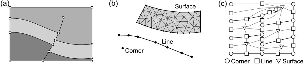
(a) Geological 2D models are defined by a geometry and a topology. (b) The geometry is set by the geometrical discretizations (meshes) of the model entities: the Surfaces, the Lines and the Corners. (c) The topology corresponds to the boundary/incidence relationships between model entities.
2 Definitions
2.1 2D geological models
In this paper, we refer to geological maps and geological cross-sections by the generic term of 2D geological models (Fig. 1a). 2D geological models are defined by Surfaces representing cross-sections in geological layers. They are delimited by the Lines that represent geological interfaces (e.g., horizons, faults, unconformities) and by Corner points representing interface contacts (e.g., fault–fault, fault–horizon) and fault tips. Model Surfaces, Lines and Corners are called model entities. This definition follows the RINGMesh library (Pellerin et al., 2017) on which our implementation is based.
The geometry of the model is determined by the geometry of all its entities (Fig. 1b). The incidence relationships between these entities define the topology (or connectivity) of the model (Fig. 1c).
2.2 2D model validity
To ensure the correctness of most operations made on a 2D model, this model must be valid. The validity of a geological model is defined by a set of criteria on its topology, its geometry, and the consistency between topology and geometry. This section summarizes the rules we use to verify that a geological model is valid. Since the model Surfaces are defined and controlled by their boundary Lines and Corners, validity conditions are formulated as criteria on the model Lines and Corners.
Topological validity. Topological validity conditions are strong validity criteria ensuring model integrity (Mäntylä, 1988; Requicha, 1980; Sakkalis et al., 2000). The relationships between model entities are constrained to ensure a valid topology for a geological model. In our case, the topological validity conditions on 2D models are: (1) a Corner should have at least one incident Line, and (2) a Line should have exactly one (closed Line) or two boundary Corners.
Depending on the modeled geological element, these constraints can be stronger. A Corner has only one incident Line if and only if the Line represents a fault (Caumon et al., 2003). Such Corners are called free Corners and correspond to fault and fracture tips.
Consistency between topology and geometry. The model geometry should be consistent with the model topology. The intersections between two entities must be a subset of their boundaries (Requicha, 1980). As a consequence, two neighboring Lines must share the same Corners at their common extremities (Fig. 2a), and there can be no intersection between two Lines representing conformal horizons (Fig. 2b).
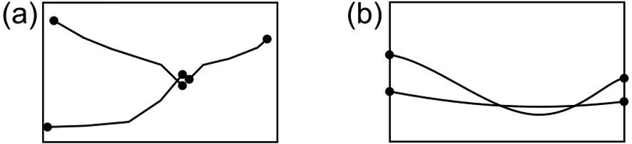
Typical invalid configurations breaking consistency between model topology and geometry are (a) non-conformity between adjacent Surfaces and (b) intersections between Lines.
Geometrical validity. We define criteria on the shapes of model entities (Fig. 3a). These criteria rely on the definition of minimal entity local sizes (i.e. Line lengths, Surface local widths that are equivalent to the distance between surface-boundary Lines) and the minimal angles between two adjacent Lines. These validity criteria depend on the requirements of numerical methods run on the model. As Surface meshes are constrained by the model interfaces, these criteria on model entities aim at improving mesh quality metrics such as minimal angle or minimal edge size (e.g., Shewchuk, 2002), and at improving the accuracy of the computations as well as the simulation computation time.

Geometrical invalid features. (a) Entity invalid configurations. (b) Mesh invalid configurations.
We use also validity criteria on the discretization of model entities (Fig. 3b). The meshed entities should have a valid mesh, i.e. composed of non-empty triangles with edges that intersect properly (see Frey and George, 2000, for extended definitions).
Entity exclusion zones to define geometrical validity. To detect geometrical invalid features, we define for each model Corner and Line ei an exclusion zone from a given minimum distance and minimum angle at Corner (Fig. 4). Exclusion zones are defined implicitly using distances to the entity ei to determine if a point belongs to the exclusion zone or not. Exclusion zones represent areas that cannot overlap other entity exclusion zones and which should not include, even partially, any other model entity. More formally, we can write the geometrical validity condition between two model entities as:
| (1) |

Detection of invalid model zones from the intersections of exclusion zones defined around the model entities. Notice that the two criteria are combined: the angle criterion is combined on the tips of exclusion zones in (a).
where is the set of model entities and Z(ei) is the exclusion zone of the model entity ei. The intersections between exclusion zones define invalid features of the input model (Fig. 4, right).
Input minimal entity sizes and minimal angles may vary spatially and from one entity to another, depending on available data, physical properties, or prior knowledge on the importance of each model feature for the application. As a consequence, the thickness of the exclusion zones, which is deduced from these input data, is not necessarily constant. Note that an exclusion zone Z(ei) can be reduced to the entity ei itself, locally or everywhere (no condition about angles and local sizes).
3 Proposed approach
Our main objective is to generate a 2D geological model that respects validity conditions from an invalid input model. In addition to the input model, a desired minimal mesh size and minimal angle are given as input parameters. These geometrical parameters define an exclusion zone for each model Corner and for each model Line. Prior geological knowledge, e.g., the type of contact between layers (conformable or not), may additionally be used to constrain the model-editing strategy.
3.1 Elementary model editing operations
To remove the identified invalid model features, we perform elementary operations that are only geometrical operations or both topological and geometrical operations (Fig. 5).
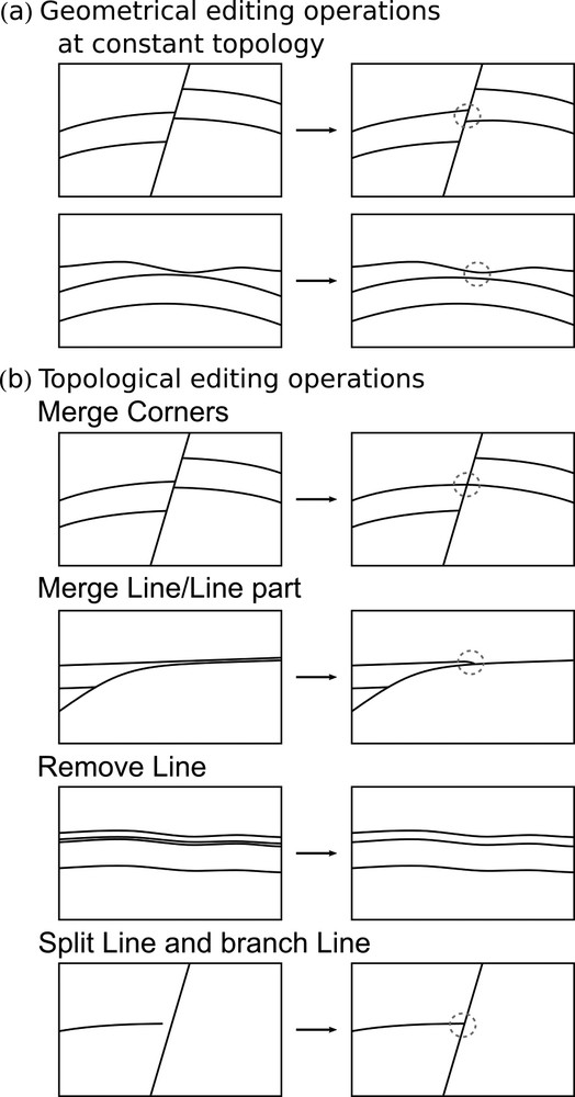
The most common geometrical and topological operations performed to fix geological cross-sections.
The two geometrical operations, model feature reshaping and mesh editing, do not change the model topology (Fig. 5a); they aim at thickening or enlarging small model features. The three topological operations, entity merging, entity splitting, and entity removal, modify the number of model entities and their connectivity (Fig. 5b); they aim at deleting thin model features by collapsing them. These operations reduce the topological model complexity (Pellerin et al., 2015).
3.2 Overview
We introduce a graph, named invalidity graph G, to support our method. The graph G stores at each step the necessary information needed to solve the editing problem. The input geological models are edited in three steps (Fig. 6).
- 1. Analysis of the input model and detection of the topological and the geometrical invalid features (Section 4.1). They are stored in the graph G.
- 2. Determination of the editing operations to perform (Section 4.2). These corrections are made on the graph G and formulated by elementary graph operations.
- 3. Reconstruction of the output geological model. The edited graph G is interpreted in geometrical terms: the topology of the edited model is first determined, and then the geometrical embedding corresponding to this topology is found (Section 4.3).
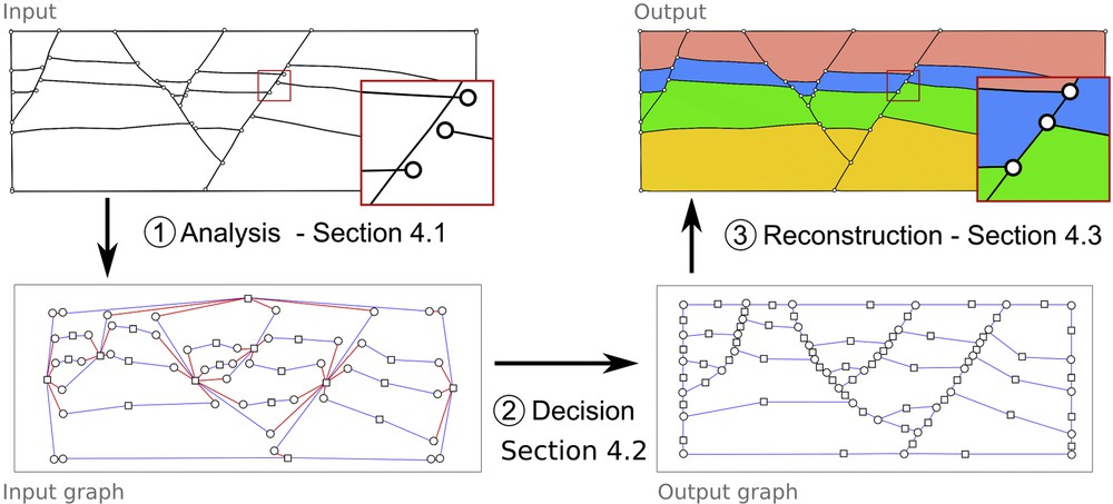
Workflow of our geological model-editing approach using an invalidity graph.
Our strategy disconnects graph editing from geological model editing. The advantage is that the decision-making about corrections, performed into the graph G, is (i) performed only after having identified the invalid features, and (ii) decoupled from effective model modifications. It allows applying the modifications only once after all correcting decisions have been made. The input model is thus kept as a reference model to avoid a too large difference after modifications. Moreover, it avoids mixing topological and geometrical changes that often lead to instabilities or inconsistencies (e.g., Euler et al., 1998; Pellerin et al., 2014).
3.3 Problem formulation using a graph
The invalidity graph G is a key point of our method: (i) it is a simple abstract representation storing the invalid configurations as graph edges, (ii) it supports the formulation of elementary model editing operations as successive elementary graph operations, and (iii) it disconnects decision making about model editing from the implementation of the modifications: the decisions are made on the graph before being performed on the geological model.
Graph definition. We define the invalidity graph G = (N,E) where N denotes the set of graph nodes and E denotes the set of undirected graph edges (Fig. 7). A model entity type (either Corner or Line) is assigned to each graph node Ni ∈ N. In addition, we assign to a graph node Ni the set of input model parts the node represents, denoted by p(Ni). For example, a graph node colored as a Corner node, can represent two input model Corners and one part of an input model Line.
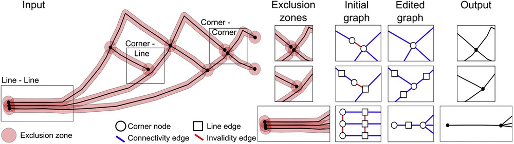
Input geological model entity exclusion zones are used to detect issues. These issues are then represented by invalidity edges (in red) in the graph G. Then, the graph G is edited to remove the red edges, which provides information for output reconstruction.
There are two kinds of edges in E. First, the edges in the subset Ec represent incidence–boundary relationships between nodes (blue edges in Fig. 7). Second, the edges in the subset Ed represent invalid configurations between nodes (red edges in Fig. 7). A graph edge Ed(A,B) between nodes A and B is also associated with a property, denoted p(Ed(A,B)), which stores the input model entity parts of A and B where their exclusion zones intersect. Note that p(Ed(A,B)) ⊂ (p(A) ∪ p(B)).
Problem reformulation. Invalid configurations are represented by the set of edges Ed. Correcting the model thus consists in the removal of all the invalid edges Ed. The graph is said valid when the set Ed is empty. Removing the invalid edges Ed implies modifications on the graph G that are then translated into modifications on the geological model.
4 2D model correction and simplification method
4.1 Analysis of the input model
In this first step, the input model is examined to detect the configurations breaking its validity and thus to initialize the graph G. The graph is initialized by first creating one node for each model Corner and each model Line. At initialization, each node representing a model Line corresponds to this Line from its first boundary Corner to its last boundary Corner. The connectivity edges Ec are set with respect to the input model boundary–incidence relationships.
Edges Ed are added into the graph G (Fig. 7) whenever an invalid configuration is detected. Topological issues, such as horizon free borders, are detected by inspecting the graph of entity connectivities. A geometrical search is performed to find the nearest model entity Enearest to which the free Corner Cfree should be connected. The nearest model entity is determined by using the anisotropic distance function induced by the free Corner exclusion zone (i.e. the convex gauge function, see Appendix A for definitions). An edge Ed(Cfree,Enearest) is added between the node representing Cfree and the one for Enearest.
For intersections between the exclusion zones of two model entities ei and ej, an edge Ed(Nei,Nej) is added between two nodes and (Fig. 7). The property on this edge, p(Ed(Nei,Nej)), corresponds to the set of points of the entities where Z(ei) and Z(ej) intersect.
In our implementation, the exclusion zone of a Line is equal to the union of the disks centered on all the points of the Line. This definition is equivalent to the definition of the dilation of the Line by a disk in mathematical morphology (e.g., Serra, 1986). The exclusion zone of a Corner is given by corner dilation by a chosen convex shape (e.g., disks, ellipses, rectangles). In this process, the use of an ellipse or a rectangle whose main axis is aligned on the Line incident to the Corner makes it possible to detect free Corners that are close to another Line. Intersections between exclusion zones are easily detected by computing convex shape intersections, e.g., using the GJK algorithm (Gilbert and Foo, 1990). We identify all the entity points (not only its vertices) whose corresponding disks (or convex shapes) compose the intersections between exclusions zones. These identified points are recorded in the property of the corresponding invalidity graph edge. The detection of intersections can be implemented using exact predicates (e.g., Lévy, 2015) for increased robustness.
4.2 Elimination of graph invalid edges
The goal of this step is to determine how to correct invalid configurations, i.e. how to edit G to remove all edges of Ed. We perform successive graph elementary operations to remove all the invalid edges (Fig. 8). These graph operations correspond to operations on the geological model.
- 1. Edge deletion. The edge between A and B is removed without affecting A and B (Fig. 8a). This operation corresponds to a geometrical editing of the model without modification of its topology.
- 2. Edge contraction. The edge between A and B is removed by merging A and B (Fig. 8b). This operation is only performed between nodes of the same entity type and corresponds to the merger of two geological model entities.
- 3. Node removal. One node is removed, leading to a removal of the incident edges (Fig. 8c). This operation corresponds to the removal of a geological model entity considered as unimportant or a duplicated model feature. Prior geological knowledge, given as input, is required to determine which node is removed.
- 4. Node splitting. One node is split into two new nodes (Fig. 8c). This operation can only be performed on a node representing a Line and corresponds to the subdivision of a model Line in two connected parts. This leads to the removal or redistribution of the incident edges.
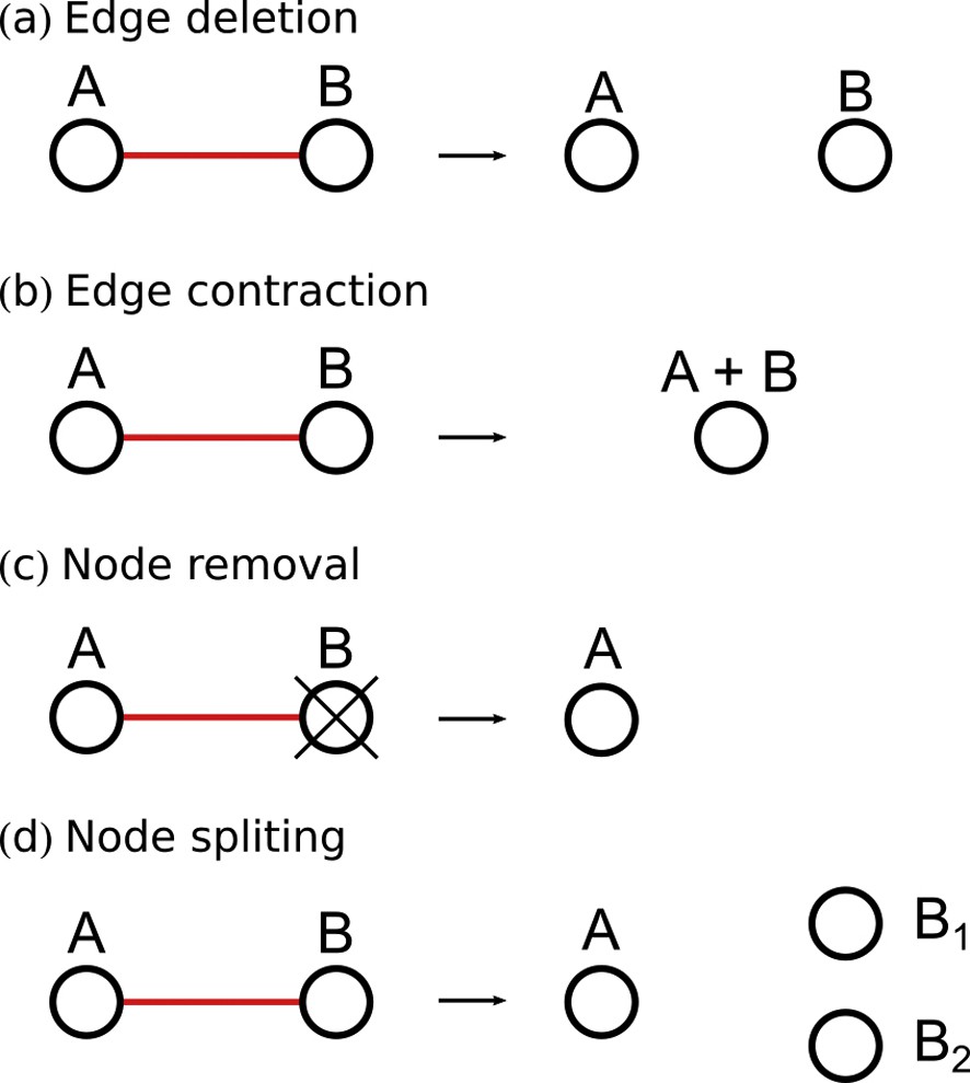
The four elementary graph operations performed for removing invalid edges (Ed) from the graph G.
The different options are constrained by (i) the entity type of the nodes (see Appendix C), (ii) the selected editing strategy given as input (e.g., seeking either preservation or simplification of model connectivity), (iii) the geological types of the entities, e.g., edge deletion cannot solve horizon free-border invalid configurations.
We first process the edges between a Line node and a Corner node and then the other edges. This choice is motivated by the fact that Line-Corner is the most frequent configuration for horizon free-border invalid edge. Starting with this configuration allows tackling first the potential non-conformity repair problem, and then the simplification one. Because the collisions of Line exclusion zones may not concern the whole Lines, operations on Line-Line invalid edges like edge contraction or node removal may need, as a pre-process, node splitting (see Appendix B).
4.3 Reconstruction of the geological model
The graph G contains all the information needed to generate the output model. The nodes N and the set of incidence edges Ec directly define the output model topology. Each graph node is converted into an output model entity and each graph connectivity edge is translated into an entity incidence–boundary relationship. For determining the geometrical embedding of the model entities, the node properties p(Ni),∀i ∈ |N| contain the lists of input model entity parts that should be used as input.
In our approach, Corners are first geometrically set and then Lines are resampled between their bounding Corners. The position of the output Corners is determined depending on the input model entities listed in the corresponding node property. If a node property is only composed of input Corners, the geometric position of the new Corner is set at the barycenter of input Corners. However, if a node property includes also input Line parts, the given barycenter of input Corners is projected on each input Line part and finally the new Corner is set at the barycenter of these projected points. This avoids, for instance, the generation of kinks on fault traces when connecting a horizon free extremity. Once Corners and Lines have been resampled, it is possible to compute the number of surfaces composing the output model and to retrieve the boundary relationships between Lines and Surfaces. The Surfaces can be meshed using various tools, e.g., Triangle (Shewchuk, 1996), Gmsh (Geuzaine and Remacle, 2009) or mmg2d (https://www.mmgtools.org/).
5 Application
A practical difficulty in the application of the proposed method is to choose the appropriate level of model simplification to preserve the accuracy of physical computations. To investigate this problem further, we propose a preliminary sensitivity study: we start from an invalid model and perform a model topological repair (Section 5.1) without geometrical simplification, then we perform model simplifications and analyze the impact on wave propagation simulations (Section 5.2).
5.1 Sealing of a 2D geological model
In this first application, we repair a non-watertight vertical cross-section from a 3D geological surface-based model built by Collon et al. (2015); this model represents a restricted area of the Lorraine coal basin (northeastern France). The original 3D model describes the geological regional structures (13 faults and 2 horizons) and 71 sub-vertical coal beds (Fig. 9) modeled by triangular surfaces. A north–south cross-section almost perpendicular to the Saint-Nicolas fault is extracted from this 3D model. The 2D cross-section is composed of 246 Corners and 126 Lines representing the Saint-Nicolas fault, the topography, the Permo-Triassic base horizon, and the 71 coal beds (Fig. 10a). The cross-section in Fig. 10a shows that the model is not watertight; there are small gaps and overlaps at contacts between coal bed Lines and fault Lines and boundary Lines. These issues are due to the remeshing of coal bed surfaces during the building of the 3D geological model (Collon et al., 2015).
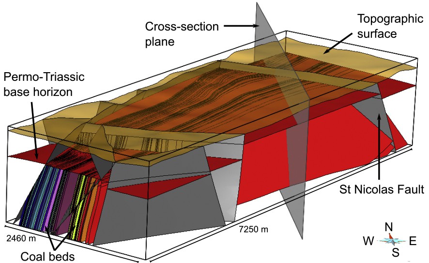
3D geological model around the Merlebach mine (North-East France) built by Collon et al. (2015) and composed of surfaces for horizons, faults and coal beds. The grey north–south surface is the vertical plane supporting the 2D cross-section.
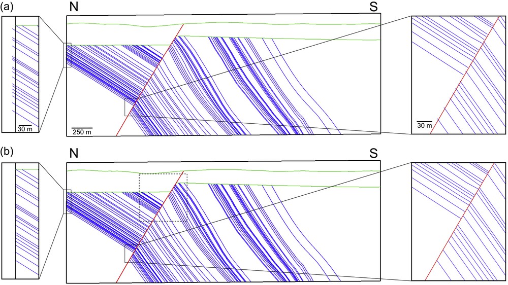
(a) Input non-watertight cross-section (note the gaps and the overlaps on detailed views). (b) Sealed output cross-section. Gaps and overlaps have been removed, resolving non-watertightness features. The dotted lines represents the sub-domain on which we run wave propagation simulations.
To seal the 2D model, we apply our graph-based approach. Minimal local entity size and minimal angle values are set to zero because the objective is only to repair this model without simplification. Moreover, we use additional geological knowledge: the coal veins are conformable one to another. This constrains our method by preventing mutual branching of vein Lines. As a consequence, vein free borders can only be connected to the fault, to the Permo-Triassic base horizon, or to a boundary Line. The generated output 2D model (Fig. 10b) is watertight. As correcting these topological issues involves line splitting operations, the number of model lines evolved from 126 to 367. The execution time for repairing this cross-section is 0.17 s on a laptop with a 2.50 GHz processor Intel®Core™ i7-6500U.
5.2 Impact of 2D model simplification on wave propagation
The objective of this second application is to show that we are able to slightly simplify a model without significantly changing the results of seismic wave propagation simulations. This is possible by directly using physical parameters from seismic wave simulations as input of our method.
Definition of a velocity model. From the geometrical model, we extract a sub-domain on which acoustic wave propagations are run. These simulations are performed using a velocity-stress formulation finite-difference method on Cartesian grid (Virieux, 1984) in 2D. In the Merlebach area, coal beds thicknesses vary from a few centimeters to 5 m (Collon et al., 2015); for simplicity, model lines representing coal beds are rasterized by setting a constant vein thickness of 1 m. We set the grid size equal to 0.33 m; thus each coal bed is represented by oblique rows of three cells. The grid dimensions are 1800 cells by 1800 cells, covering the 600-m-by-600-m sub-domain represented by the dashed line in Fig. 10b. We define three rock domains (Fig. 11a): the Permo-Triassic conglomerates at the top (P-wave velocity = 3 000 m·s−1, in blue in Fig. 11a), the deeper Westphalian and Stephanian claystones, sandstones and conglomerates (P-wave velocity = 4 000 m·s−1, in red in Fig. 11a), and intercalated coal beds (P-wave velocity = 2400 m·s−1, in green in Fig. 11a). Note that we ignore the P-wave velocity variation with depth and that we use the constant density approximation for simplicity.
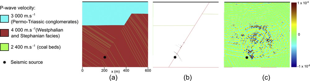
(a) Velocity model corresponding to the simplified model mout. (b) Difference between the input velocity model and the simplified velocity model δm (in black). (c) Wavefield difference δu on one snapshot (t = 0.3 s after shock).
We set a seismic source (Ricker wavelet) with a maximum wave frequency fmax = 300 Hz. As a consequence, the minimum wavelength is 8 m, which is sampled by 24 grid points. The grid sampling is considered fine enough to reduce numerical dispersion (at least 10 grid points, Virieux, 1984). The seismic resolution r is given by the quarter-wavelength criterion (e.g., Yilmaz, 2001, chapter 11):
| (2) |
Simplified model. We apply our graph-based method to simplify the generated sealed model (Section 5.1). The objective is to remove the small model features, e.g., the small lines caused by very close fault–horizon contacts. To do so, the minimal local entity size value is set to the value of the seismic resolution, i.e. 2 m (see Eq. (2)). As additional geological knowledge, we prevent mergers between coal veins precisely identified in Collon et al. (2015). As a consequence, model modifications are exclusively located at coal vein boundaries, i.e. along the Saint-Nicolas fault, the Permo-Triassic base horizon, and the model boundary (Fig. 11c). The execution time for simplifying this cross-section is 0.25 s on a laptop with a 2.50 GHz processor Intel®Core™ i7-6500U. The difference between the velocity model min corresponding to the initial geometry (Fig. 11a) and the velocity model mout corresponding to the simplified geometry is defined by δm = mout – min (Fig. 11b).
Simulations. The velocity-stress formulation finite-difference method (Virieux, 1984) used for simulations is defined with second-order accurate operators in time and eight-order accurate operators in space. We apply Perfectly Matched Layers (PML) absorbing boundary conditions (Collino and Tsogka, 2001) on the two lateral sides and the bottom of the sub-domain grid. We apply the rigid-surface condition (also called zero-displacement condition or homogeneous Dirichlet condition); see, e.g., Virieux, 1984, at the top of the domain. Waves are thus reflected on the top of the domain, simulating the reflections on the surface: the free surface is simplified to a horizontal line above the region of interest. We place one receiver by grid point at the top of the domain. The acoustic source is located on the fault, right under the location of the principal model modifications (Fig. 11). By doing so, we expect to capture the highest impact of model modifications on the recorded seismograms. Simulations are run for t = 0.5 s after the shock with a time discretization of 10−4 s. Two simulations are run: one using the velocity model min corresponding to the 2D model repaired in Section 5.1, considered as the reference, and the other one using the velocity model mout corresponding to the simplified model.
Results. We compare the difference δu between the wavefield uin simulated in min and the wavefield uout simulated in mout: we define δu = uout – uin (Fig. 11c). Using Cartesian grids is here very practical for computing the difference δu between wavefields. We also compute the RMS (root mean square) waveform difference for a given receiver using the definition by Geller and Takeuchi (1995):
| (3) |
The mean waveform difference, for all receivers, is 2.18 % with a maximal difference of 3.28 % for the receiver positioned at x = 481 m (Fig. 12). This difference is reasonably small because the modifications on the geological model have magnitudes lower than the seismic resolution r.
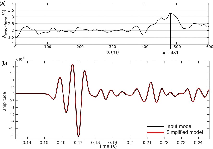
(a) RMS waveform difference as a function of the abscissa x for a maximum wave frequency equal to 300 Hz. (b) Seismograms recorded by the receiver x = 481 m (maximal RMS waveform difference). The trace from the simplified model (red) is almost identical to the trace from the reference model (black).
To check the impact of the same simplifications on higher-frequency wavefields, we ran additional simulations: we kept the same parameters, but doubled the wave frequency (fmax = 600 Hz). Using this frequency, the minimum wavelength is 4 m, which is sampled by 12 grid points, and the seismic resolution r (Eq. (2)) is now around 1.00 m. Using fmax = 600 Hz, the difference on the full waveforms is now 12.45 %, with a maximal difference of 19.44 % for the receiver positioned at x = 438 m (Fig. 13). The wave propagation differences are significantly higher at this frequency, as expected, since the magnitude of the simplifications on the geological model (i.e. 2 m) is larger than the seismic resolution (i.e. 1 m).
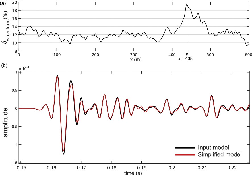
(a) RMS waveform difference as a function of the abscissa x for a maximum wave frequency equal to 600 Hz. (b) Seismograms recorded by the receiver x = 438 m (maximal RMS waveform difference). The trace from the simplified model (red) has more difference from the trace from the reference model (black) than for a 300 Hz source wavelet.
6 Discussion
Geological model simplifications impact physical simulations, but we have shown that the effects can be reduced to an acceptable amount (below 4% in our example for fmax = 300 Hz) by constraining the magnitude of geological model modifications below the spatial resolution imposed by the simulated physical phenomena. If the magnitude of modifications is bigger than the seismic resolution, the difference is significantly bigger (more than 10% in our example for fmax = 600 Hz). In the proposed method, this magnitude is directly controlled by the size of the entity exclusion zones set as input of the method. As a consequence, it is possible to use prior knowledge about the wavefield frequency content to choose the simplification parameters that have a negligible impact on the simulation results.
The presented application shows simulations performed using a Finite Difference scheme on Cartesian grids. This is intentionally a very simple application, using a common FD scheme and simple velocity models. We have shown that it is possible to use as input of our method the physical parameters of the simulation to limit the impact of simplifications on simulation results.
However, because the two grids have the same dimensions, we cannot measure on this application the benefits of simplifications on simulation run time. To go further, the FD scheme can be improved using methods accounting more for discontinuities of the models (e.g., Kristek et al., 2016; Moczo et al., 2002). Another possibility is to explicitly adapt the spatial discretization to the model discontinuities using 2D unstructured meshes. By doing so, P-SV wave propagation simulations can be run on 2D unstructured meshes using Discontinuous Galerkin scheme (e.g., Käser and Dumbser, 2006; Peyrusse et al., 2014), or triangular Spectral Elements (e.g., Mercerat et al., 2006). This would allow comparing both the simplification effects on simulation accuracy, but also on computation time directly on the generated unstructured meshes, without any rasterization step.
7 Conclusion
The proposed framework to edit 2D geological boundary models eases model editing by automatically detecting the invalid configurations and correcting them. This method can be used to correct the issues breaking the unphysical watertightness of 2D geological models. It is also able to simplify model interface geometries and connectivity to improve the quality of the generated meshes.
We have shown that, for the problem of wave propagation, our simplification method has a limited impact on the simulation results, provided that the amount of simplification is small with regard to the sensitivity of the physical simulations. This condition can be checked in seismic applications for which minimal velocity and maximum frequency are known. However, the choice of the simplification size cannot be easily expressed for all physical processes such as fluid flow and transport. In that case, our method makes it possible to experiment numerically different magnitudes of simplification and to measure their impact on the considered physical process.
Moreover, our method is can be customized to include prior geological knowledge by adapting the simplification strategies to preserve the geological model features deemed essential. This opens interesting perspectives to adapt the simplification strategies both in terms of prior knowledge and in terms of sensitivity of the physical problems.
However, the present version of the method cannot detect unsolvable configurations given input parameters on minimum angles and minimal feature sizes (e.g., when a stack of horizon lines are much closer than the input minimum feature size). In some cases, invalid configurations may still be present after the application of the method. In some pathological cases, the whole procedure should, therefore, be executed several times, and the exclusion zones may need to be reduced to obtain an output model that conforms to the given validity criteria.
Our ultimate objective is to extend the proposed method to repair and simplify 3D geological models. Extension to 3D of any geometrical operations is always extremely difficult. Model editing is highly non-trivial because many 3D geometrical operations are difficult, while the corresponding 2D operations are simple and well understood, e.g., mesh generation. However, we do believe that the dissociation between topological operations and geometrical operations that we propose is key for a successful 3D simplification method. The main challenge will be to fix the 3D geometrical embedding once the topology is fixed.
Acknowledgments
This work was performed in the frame of the RING project at the Université de Lorraine. We thank for their support the industrial and academic sponsors of the RING–GOCAD Consortium managed by ASGA (http://www.ring-team.org/consortium). J. Pellerin is supported by the European Research Council, grant agreement ERC-2015-AdG-694020. Software corresponding to this paper is available to sponsors in the RING software packages SCAR (model editing) and SIGMA (wave propagation simulations). We acknowledge E. Chaljub, M. Karimi-Fard, and N. Glinsky for their constructive remarks that helped us to improve the quality of this paper. The authors would also like to thank Arnaud Botella for fruitful discussions. The authors acknowledge INRIA for the Geogram library used in RINGMesh and Paradigm for the SKUA–GOCAD software.