

1 Introduction
Mountainous glacial valleys commonly exhibit characteristic parabolic or "U"-shape transverse sections which are extensively studied and discussed in the literature (Augustinus, 1995; Harbor, 1990; Harbor et al., 1988; Hirano and Aniya, 1988; Montgomery, 2002). On the contrary, the longitudinal shape of glacial valleys is generally more cryptic: it can show successive steps, overdeepened basins, winding substratum geometry, and hanging tributary valleys (Anderson et al., 2006; MacGregor et al., 2000; Penck, 1905). After the eventual glacial retreat, the overdeepened basins are generally filled progressively with glacial, lacustrine, and/or alluvial sediments. The sedimentary infill thickness may reach dozens to several hundreds of meters, and remains often poorly known.
In the Pyrenees mountain range (located between France and Spain, Fig. 1a), successive glaciation/deglaciation phases and strong climatic contrasts during the Quaternary caused a very heterogenous ice cover at regional scale (Calvet, 2004; Stange et al., 2014). The main glaciers (75% of total ice cover) affected the northern central section of the ridge (Taillefer, 1984), with glacier tongues spreading to the mountain front and forelands (Calvet, 2004; Hérail et al., 1986; Taillefer, 1969). The Aure valley (France, Fig. 1b) is a major alluvial valley in the central part of the Pyrenees spreading from the French–Spanish border to the city of Lannemezan. Between the Saint-Lary and Cadeac towns, the valley widens into a kilometre-wide flat basin, suggesting glacial carving into the substratum, later filled by sediments (Fig. 1b). The sediment thickness within the Aure valley remains badly constrained, although it is a critical information, e.g., for erosion process studies (Hinderer, 2001; Schrott et al., 2003), geotechnical engineering design (Foged, 1987), hydrological (e.g., municipal water stock estimation) surveys (Preusser et al., 2010) or seismological site amplification estimation (Aki, 1993; Dubos et al., 2003; King and Tucker, 1984).

a) Map showing the maximal glacier extent in the Pyrenees (cold blue area, from Calvet et al., 2011). The area of this study is delineated by the red rectangle. Valley names are shown in blue. b) Geological map of the study area (modified from Mirouse and Barrère, 1993). Continuous and dashed black lines delineate the main faults. The Soulan Fault (SF) is delineated by a thick dashed line. Thrust faults are shown as continuous black lines with triangles. The legend for the geological units is given at the bottom of the figure. The drilling in Saint-Lary is indicated by the black star. Rivers are shown by solid blue lines. Northern (NB) and southern basins (SB) are shown on the map. c) Location of survey measurements. Gravimetric measurements located on top of the sediment body are indicated by white squares, while stations located on the bedrock are marked with grey squares. Note: gravity stations located far from the study area are not shown in the figure. Passive seismic measurements belonging to D1 and D2 datasets (reliable measurements) are indicated by orange diamonds. Unreliable stations are shown in red. The drilling in Saint-Lary is indicated by the black star. Rivers are shown by solid blue lines. Masquer
a) Map showing the maximal glacier extent in the Pyrenees (cold blue area, from Calvet et al., 2011). The area of this study is delineated by the red rectangle. Valley names are shown in blue. b) Geological map of the ... Lire la suite
Geophysical methods represent low-cost and non-invasive tools to map such sediment infill. For example, geological structures are known to cause seismic resonance due to geometrical effects or impedance contrasts (Bard and Bouchon, 1980a, 1980b; Pischiutta et al., 2010; Spudich et al., 1996). Such resonance phenomena can be observed using ambient vibration records and may be used for various applications such as landslide monitoring (Bottelin et al., 2013a, 2013b; Mainsant et al., 2012), structural health assessment of civil engineering structures (Michel et al., 2008; Mikael et al., 2013) or site effect characterization (Aki, 1993; Lermo and Chavez-Garcia, 1994). The resonance frequency f0 of a soft geological layer overlying the bedrock can be derived from the ambient vibration Horizontal to Vertical Spectral Ratio (HVSR) (Field et al., 1995; Haghshenas et al., 2008; Lachet et al., 1996; Nakamura, 1989). This passive method allowed cheap and practical surveys (Souriau et al., 2011) and was extensively used for prospection purposes over the last twenty years (see review from Mucciarelli and Gallipoli, 2001). A gravimetric method was also used in the literature to estimate the substratum geometry in glacial valleys (Barnaba et al., 2010; Møller et al., 2007; Perrouty et al., 2015; Rosselli and Olivier, 2003). The sediment thickness can be derived from gravity measurements provided that sufficient density contrast exists between sediment layer and the bedrock (Kearey et al., 2013). However, both methods struggle to discriminate between successive deposit bodies (e.g., glacial, fluvio-glacial or fluviatile deposits) because of close seismic properties and densities. Geoelectrical methods and refraction surveys were successfully used to image the infill body in shallow (tens of meters) basins in the North of Spain (Turu et al., 2002; Vilaplana, 1983). Such techniques yet imply low ratios between the investigation depth and the profile length at surface, facing rapid limitations when the bedrock depth increases (Turu i Michels et al., 2007).
This article aims at mapping the bedrock topography of the Saint-Lary basin (northern central Pyrenees, France) by means of single station ambient vibration (HVSR) and gravity surveys. Each method is processed separately, after which a joint interpretation is proposed. This bedrock map represents a useful input for further local and regional studies such as Quaternary surveys, seismic microzonation, or municipal water resource estimates. Finally, we explore some geomorphological processes that may explain the Saint-Lary basin shape.
2 Geological, geotechnical, and geomorphological settings
The study area is located in the northern central area of the Pyrenees mountain range, France (Fig. 1a). The Saint-Lary basin lies in the middle section of the Aure valley, which carves the mountain range over about 40 km along a SSW–NNE direction. The Saint-Lary basin is ~1 km wide and ~10 km long. The Soulan fault delineates the southernmost part of the basin (Fig. 1b). The outcropping bedrock is composed of Devonian quartzite and shale from La Munia Unit (Mirouse and Barrère, 1993). The substratum at the northern part of the Soulan fault is composed by highly folded Carboniferous limestone, sandstone, and black shales flysch series. Limestone and shale from the Chinipro Unit surrounded by Jasper rocks crop out in the larger anticlinal folds (Fig. 1b). North of Ancizan and south of the city of Cadéac, the basin narrows, crossing the subvertical limestone of Chinipro Unit affected by the contact metamorphism of the Bordères–Louron granite (Barrère et al., 1984). In the remaining of this article, the southern basin area located between the Saint-Lary and Guchan towns is defined as the southern Saint-Lary basin. The northern area located between Guchan and Cadéac is defined as the northern Saint-Lary basin.
During the Pleistocene, the Pyrenees endured major glaciations, whose timing and pattern remain debated (Calvet, 2004; Penck, 1885; Taillefer, 1967). The maximum glacial extent in the Pyrenees (Fig. 1a) may have occurred during the Marine Isotope Stage MIS 4 (70–50 ka BP) or simultaneously with the global Last Glacial Maximum (LGM, ~MIS 2, 23 to 19 ka BP) (Calvet et al., 2011; Delmas et al., 2012; Mix et al., 2001; Pallàs et al., 2006). In the Aure valley, evidences of glacial activity suggest that the ice covered the valley until the city of Ancizan, only occasionally overstepping the Cadéac rock bar and never reaching the city of Arreau (Fig. 1b, Mirouse and Barrère, 1993). The Saint-Lary basin was then filled with a mix of fluvio-glacial sediments of unknown total thickness.
Most of the boreholes in the area were conducted for geotechnical purposes and, unfortunately, range only from a few meters to about 20 m in depth. They dug only superficially into the fluvio-glacial sediment deposit, which appears as a mix of sand, pebbles, gravels and blocks blended into a clayey matrix. Only one borehole drilled into the underlying substratum (http://ficheinfoterre.brgm.fr/InfoterreFiche/ficheBss.action?id=BSS002MJUL, accessed October 2018) provided a local information about the sediment fill thickness (black star in Fig. 1b and c). It showed a 120-m sedimentary layer (without more details) lying over the substratum (black shales and limestones from the Devonian La Munia Unit).
3 Passive seismic study
3.1 Measurements
Seismic noise was recorded at 69 stations throughout the Saint-Lary basin (diamonds in Fig. 1c). For each station, ambient vibrations were recorded during at least 40 min with two 3C seismic sensors: one broadband Güralp CMG40T (eigenperiod of 30 s) and one short-period IHR 3D (eigenfrequency of 2 Hz) (http://sismob.resif.fr), the latter levelling off faster. Seismic streams were acquired using an Agecodagis Osiris unit sampling at 100 Hz with an embedded 50 Hz anti-alias filter. Ambient vibrations were then processed through Geopsy software (www.geopsy.org). We subtracted the mean and trend of each seismic trace before applying a 0.1 Hz high-pass filter. Transients were eliminated using a STA/LTA algorithm (Trnkoczy, 2002) before cutting the ambient vibration stream into 25-s-long tapered windows to reduce its statistical variability (Picozzi et al., 2005). The Fourier spectrum was then computed for each window and smoothed with a Konno–Ohmachi filter (Konno and Ohmachi, 1998) using b = 40. The horizontal component is computed as the quadratic mean of the north and east channels. The Horizontal to Vertical Spectral Ratio (HVSR) is computed for each window, yielding mean curve (MHVSR) and standard deviation (σHVSR) for each station (Fig. 2).
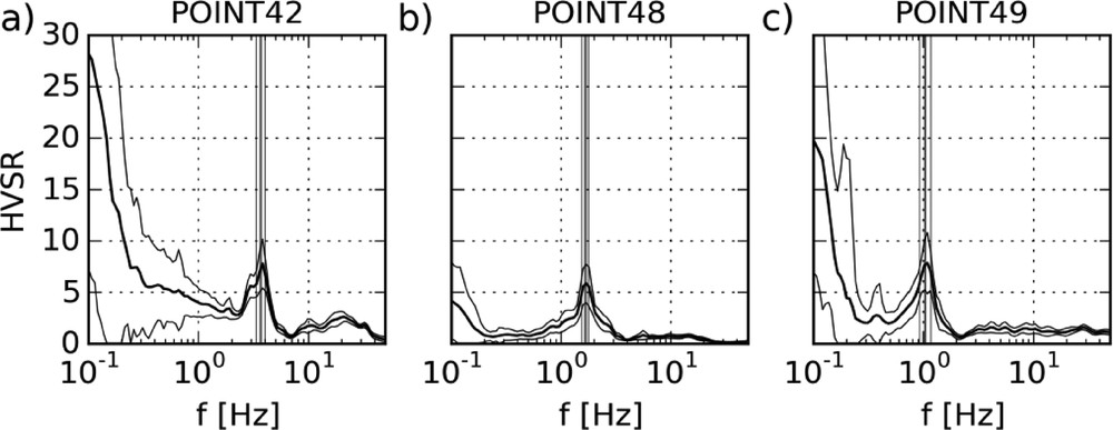
HVSR curves for three measurement points. The mean HVSR curve (MHVSR) is shown by a thick black line. MHVSR/σHVSR and MHVSR × σHVSR curves are drawn with thin black lines, σ being the standard deviation. The frequency of the HVSR peak (f0) is indicated by the thick vertical grey line. f0 ± σ(f0) limits are drawn with thin grey lines. Fig. 2a and c illustrate the high HVSR observed at low frequency due to environmental conditions (wind effect). Fig. 2b and c show peaks matching the SESAME guidelines' criteria. Masquer
HVSR curves for three measurement points. The mean HVSR curve (MHVSR) is shown by a thick black line. MHVSR/σHVSR and MHVSR × σHVSR curves are drawn with thin black lines, σ being the standard deviation. ... Lire la suite
3.2 Results
Eleven unreliable measurements (red diamonds in Fig. 1c) were eliminated because of non-compliance with SESAME standards (SESAME, 2004). They were mostly affected by strong transients or instrument malfunction. In the remaining set of measurements (orange diamonds, Fig. 1c), the peak detection operated in the 0.5–50 Hz frequency range, where the basin resonance is likely to occur. Peaks located lower than the sensor eigenperiod were not taken into account for confidence reasons (Guillier et al., 2008). Most points exhibit high HVSR at low frequency (<0.5 Hz, see Fig. 2a and c). This feature is likely related to wind effects, as a strong valley breeze blows in the area (Chatelain et al., 2008; Mucciarelli et al., 2005; SESAME, 2004). Soil cover such as pavement can also contribute to such peculiar HVSR pattern (Bonnefoy-Claudet et al., 2009). Among the HVSR dataset, 18 points met the SESAME engineering criteria (dataset D1, SESAME, 2004). Most of the stations yet did not fulfil the SESAME peak amplitude requirements because of the high HVSR level at low frequency. A closer analysis of seismic noise spectra was conducted, allowing us to spot a clear drop in vertical component energy for additional 35 points (dataset D2). The remaining points show complex or multiple peaks and were not further used in this study (dataset D3). The clear HVSR peaks from D1 and D2 were interpreted as seismic resonance effects in the Saint-Lary basin. The frequency of the first peak is then an estimate of the basin fundamental resonance frequency f0, which results from wave trapping in the sediment layer (Nakamura, 1989). This assumes a large-enough impedance contrast between the superficial normally consolidated sediment fill and the underlying bedrock, in good accordance with the geological settings of the Saint-Lary basin (see Section 2). The resonance frequency f0 is mapped for each measurement station in Fig. 3a and b. f0 ranges from 0.8 to 21 Hz and draws a clear spatial pattern: high f0 values (>5 Hz) gather in the northern Saint-Lary basin and close to valley edges whereas lower f0 (<5 Hz) lie mostly in the southern basin. Lower f0 values are generally observed along the valley central axis and increase towards the valley edges.

Top row: passive seismic. a–b) Map of f0 frequency in the Saint-Lary basin, with linear and logarithmic colour scale, respectively. c) Map of sediment thickness H in the Saint-Lary basin. The sediment thickness was computed with the 1D formula (Eq. (1)) and VS = 845 m/s. The location of HVSR stations is indicated by diamonds. Bottom row: gravity measurements. d) Complete Bouguer anomaly. e) Residual Bouguer anomaly. f) Sediment thickness in the Saint-Lary basin. The density contrast was set to 300 kg m−3. The location of gravity measurement stations is indicated squares. The northern (NB) and southern Saint-Lary basins (SB) are shown in bold italics. Masquer
Top row: passive seismic. a–b) Map of f0 frequency in the Saint-Lary basin, with linear and logarithmic colour scale, respectively. c) Map of sediment thickness H in the Saint-Lary basin. The sediment thickness was computed with the 1D ... Lire la suite
In such a sediment-filled basin, the resonance phenomenon can originate from 1 D, 2 D, 3 D effects or a mix of them (Barnaba et al., 2010; Cornou and Bard, 2003; Guéguen et al., 2007; Le Roux et al., 2012; Lenti et al., 2009; Özalaybey et al., 2011; Uebayashi, 2003; Uebayashi et al., 2012; Uetake and Kudo, 2005). Bard and Bouchon (1985) defined a criterion based on the valley apex ratio (sediment thickness divided by valley width) to discriminate 1 D from 2 D cases. Considering the 0.2 apex ratio computed at the drilling site where the valley narrows (see section 2), we expected similar or smaller apex ratios in the wider Saint-Lary basin to the north. This assumption will be ascertained in the next section. This low valley apex ratio (≤0.2) implies that the basin resonance can be appropriately described by the 1 D resonance formula, whatever the shear wave velocity contrast with the bedrock (Bard and Bouchon, 1985). In addition, progressive variations of f0 at the hundred of meter scale and the absence of strong directional effect in the southern half of the basin also supports appropriate 1 D structure interpretation (Del Gaudio and Wasowski, 2007; Maresca et al., 2014). However, more complex HVSR appear closer to the valley slopes and in the northern Saint-Lary basin. This suggests that 2D resonance due to basin edge effects might no longer be negligible (Bonnefoy-Claudet et al., 2009; Claprood et al., 2012; Faccioli and Vanini, 2003; Frischknecht and Wagner, 2004; Guillier et al., 2006; Roten et al., 2006). In the southern Saint-Lary basin, the resonance frequency f0 shows smooth changes along valley cross sections (Fig. 3a and b). Clearer HVSR peaks gather along the valley deep axis, where the resonance is mostly 1D. On the opposite, broader HVSR peaks appear close to the basin edges and in the northern Saint-Lary basin, where greater f0 wandering appears.
For simple layer geometry (1 D case), the fundamental frequency f0 can be related to the sediment layer thickness H by the power-law equation:
| (1) |
| (2) |
Site location, shear wave velocity (VS) and maximal thickness (H) of the superficial sedimentary layer (from a literature review). SRa: seismic refraction; SRe: seismic reflection; SW: active surface wave analysis; B: borehole measurements; MA: microtremor array measurements, ER: electric resistivity, G: Gravity survey. (1)z denotes the depth.
| Location (country) | VS (m/s) | H (m) | Measurement type | Reference |
| Osaka basin (Japan) | 380–1440 | 2000 | SRe, SRa, B, MA | Uebayashi et al., 2012 |
| Tagliamento Valley (Alps, Italy) | 900 | 450 | MA | Barnaba et al., 2010 |
| Launceston (Tasmania, Australia) | <800 | 250 | MA | Claprood et al., 2012 |
| Bajo Segura basin (Spain) | 85–200 | 65 | B, MA | Delgado et al., 2000a |
| Bajo Segura basin (Spain) | 146–230 | 45 | B, MA | Delgado et al., 2000b |
| Lourdes basin (Pyrenees, France) | 300 | 30 | SRe | Dubos et al., 2003 |
| Lower Rhine (Germany) | 200–946 | 565 | B | Ibs-von Seht and Wohlenberg, 1999 |
| Rhône Valley (Switzerland) | 456–820 | 890 | SRe, SRa | Roten et al., 2006 |
| 800 | Frischknecht and Wagner, 2004 | |||
| 130–456 | >176 | SRa, SRe | (Burri, 1995 in Frischknecht, 2000 | |
| Grenoble basin (Alps, France) | 300 + 1.9 z(1) | 535 | B, SRa | Guéguen et al., 2007 |
| 300–750 | 450–650 | SRe, G | Le Brun, 1997 | |
| Séchilienne basin (Alps, France) | 300–920 | 400 | SRe, ER | Le Roux et al., 2012 |
| Ubaye valley (Alpes, France) | 250–1100 | 50 | SRe, SRa | Jongmans and Campillo, 1993 |
| Gave de Pau valley (Pyrenees, France) | 300 | 13–30 | SRa | Dubos et al., 2003 |
| 170–650 | 13–36 | SW | (Bernardie et al., 2006; Souriau et al., 2007) |
4 Gravity survey
4.1 Data acquisition
We acquired 87 gravity stations in the Saint-Lary basin and the surrounding area (blue squares, Fig. 1c) using a CG5 gravimeter (1 μGal resolution, < 5 μGal repeatability; Scintrex Ltd, 2009). The gravity dataset was completed by 112 stations operated by the International Gravimetric Bureau database (IGB, http://bgi.omp.obs-mip.fr). Hence, 61 gravity measurements are located within the Saint-Lary basin (white squares, Fig. 1c) and 136 stations are located on the bedrock (grey squares). The body tide correction (about 10–100 μGal) was directly applied by the instrument during the acquisition process. Polar effect, ocean loading, and atmospheric loading corrections lie below 10 μGal (Boy et al., 2002; Llubes et al., 2008) and can be neglected compared to the gravitational effect of variations in sedimentary thickness. To convert our relative gravity measurements into absolute values, we conducted repeated gravity measurements at the Vignec station from the IGB. We also repeated measurements at several other stations to estimate the instrumental drift. It was smaller than 0.13 mGal/day and was removed during data post-processing by a linear trend removal (Bonvalot et al., 1998; Gabalda et al., 2003).
High-precision positioning is of critical importance for gravimetric studies and represents a challenging task in such mountainous environment. Gravity station position was done using a Leica GR25 GNSS receptor as base and Topcon GB-10000 as a rover acquiring signal from Global Positioning System (GPS) and Global Navigation Satellite System (GLONASS) satellites. The acquisition time for positioning was set at 30 min at each gravity station to mitigate mountain mask effects. We set up the base receptor in an open field at the valley centre. Generally, 90% of the stations were positioned through Differential-GNSS (D-GNSS) computation. In this case, the accuracy is better than 10 cm. The 10% remaining stations were processed through Precise Point Positioning (PPP) and we removed from our study four stations that yielded a vertical accuracy larger than 34 cm.
4.2 Gravity anomaly maps
According to station elevation uncertainties, the free-air anomaly accuracy is better than 55 μGal for 90% of the measurements and better than 265 μGal for the remaining 10%. The plateau and topographic contributions were calculated with a mean bedrock density of 2.66. This average value was obtained by applying Parasnis' method to the 136 gravimetric stations located outside the Saint-Lary basin (grey squares, Fig. 1c), i.e. lying directly on the bedrock (Parasnis, 1986). For comparison, previous studies in the Pyrenean region used mean density values of 2.6 (Perrouty et al., 2015) or 2.67 (Casas et al., 1997). The topographic correction for terrain located closer than 1.5 km to the gravity station used the 5-m grid from the IGN (provided by the “Bureau de recherche géologiques and minières,” labelled DEM#1). A terrain located at a distance between 1.5 km and 40 km was modelled using a 30-m Digital Elevation Model grid from the Advanced Spaceborne Thermal Emission and Refection (ASTER) database (Kahle et al., 1991) and labelled DEM#2. Comparing the gravity station elevation measured with GNSS to DEM#1 yielded a mean vertical accuracy of 5 m at a 95% confidence level, whereas comparison with DEM#2 yielded a mean accuracy of 19 m at the 95% confidence level. The latter estimate is very close to Tachikawa et al.'s (2011) results for ASTER DEM (17 m mean accuracy at a 95% confidence level). This estimation yet ranges from less than 10 m to about 30 m, depending on the terrain's slope, its roughness, the vegetal cover, and the estimation method (Tighe and Chamberlain, 2009). Based on the DEM accuracies, a 0.2–0.6-mGal wandering is expected in topographic corrections for a bedrock density of 2.66.
Gravsoft software (Forsberg and Tscherning, 2008) was used to compute the complete Bouguer anomaly (Fig. 3d). The map shows a regional gravity trend from south to north due to crustal thickening under the Pyrenean Axial Zone (Casas et al., 1997). As this regional signal masks the local variations due to the sediment fill, it has to be removed from the complete Bouguer anomaly to obtain the residual gravity anomaly (Kearey et al., 2013; Sharma, 1997). We estimated this regional contribution using the gravity stations located outside the Saint-Lary basin, i.e. where there is no sedimentary cover (Fig. 3e). The choice of the adjustment method and its parametrization can yield substantial differences in the regional pattern estimation (Beltrao et al., 1991; Martín et al., 2011; Vallon, 1999). We choose to fit a second-order polynomial surface with least-square regularization because it yields small residual gravity anomaly values close to the valley edges (Fig. 3e). In our case, the residual gravity anomaly in the valley bottom is negative because the density of sediments is smaller than the bedrock density. Larger negative residual gravity anomaly values concentrate in the southern basin, dropping down to −3 mGal, close to the valley central axis. Smaller negative residual gravity anomaly values appear close to the valley edges. On the valley flanks, residual gravity anomaly values are positive. This pattern agrees well with studies conducted in other sediment-filled valleys (Barnaba et al., 2010; Vallon, 1999), including the nearby Gave de Pau and Garonne valleys (Perrouty et al., 2015). This strongly suggests that the residual gravity anomaly in the Saint-Lary valley originates from the presence of less dense sediment infill and that bedrock density fluctuations are negligible compared to Quaternary infill effects.
4.3 Estimation of the sediment fill thickness
The Residual Gravity Anomaly map (Fig. 3e) was used to estimate the sediment fill thickness (Fig. 3f) based on the density contrast occurring between the sediments and the bedrock (Barnaba et al., 2010; Sharma, 1997). This assumption is reasonable in our case, where poorly consolidated, glacial or fluvio-glacial sediments lie over the bedrock (see Section 2). We estimated a plausible range of densities for the sediment fill according to a literature review (Table 2) and successive tests. The best fit was achieved for a density contrast between sediment and bedrock of 300 kg m−3, which is consistent with previous studies in the Italian Alps (Barnaba et al., 2010) or in the Swiss Rhone valley (Frischknecht, 2000; Frischknecht and Wagner, 2004). This contrast also yields a bedrock depth compatible with the Saint-Lary drilling log. The influence of this parameter on the sediment thickness is discussed in Section 5.1.
Review of sediment fill density values and contrast with nearby bedrock.
| Site | Material | Method | Depth (m) | Density (kg·m−3) | Density contrast (kg·m−3) | Reference |
| Tagliamento River Valley (Alps, Italy) | Unconsolidated clays and sands | Active and Passive seismic | 0–30 | 1780–1850 | 650–720 | Barnaba et al., 2010 |
| Consolidated clays and sands | >30 | 2100 | 400 | |||
| Lateral alluvial fan | <20 | 2300 | 200 | |||
| Rhône valley (Alps, Switzerland | Quaternary sediment deposits | Geophysical survey compilation (gravimetric study and modeling, measurements on samples) | 0–900 | 1900–2200 | 200–800 |
Frischknecht, 2000
Frischknecht and Wagner, 2004 |
| Seismic surveys | 0–900 | – | 500–600 | Rosselli and Olivier, 2003 | ||
| Gave de Pau and Garonne valleys (Pyrenees, France) | Quaternary post-glacial unconsolidated sediment | Literature review | 0–300 | 2000 | 600 | Perrouty et al., 2015 (based on Rosselli and Olivier, 2003) |
| Gresivaudan valley (Alps, France) | Quaternary alluvial infill | Gravity measurements at depth and borehole calibration | 0–900 | 2100 | 500 |
Vallon, 1999
Nicoud et al., 2002 |
| – | Alluvium (wet) | Literature review | – | 1960–2000 | – | Kearey et al., 2013 |
| – | Poorly consolidated sedimentary material | Literature review | – | 1900–2200 | Telford et al., 1990 |
The inversion process was conducted using a 2.5 D finite-length right polygonal prism method using the Cady program (Godivier, 1986, see detailed description in Cady, 1980). Twenty-three east–west, 5.0-km-long transverse profiles were drawn with 300-m spacing between them. Each profile is composed of 99 gravity values extracted from the Residual Gravity Anomaly map (Fig. 3e) with 50-m spacing. We selected only the gravity points located in the valley for the inversion and assumed that the residual gravity was entirely attributable to sediment/basement density contrast. The inversion process then tuned the sediment thickness to fit the residual gravity values, yielding a residual with r2 ≈ 0.99 and Root Mean Square Error ≈0.043 mGal. The sediment thickness obtained from the inversion was then interpolated to draw the sediment thickness map (Fig. 3f). Accordingly to the residual gravity anomaly map (Fig. 3e), the sediment thickness culminates close to the valley axis and decreases towards the valley edges. The Quaternary infill thickness shows two deep areas in the southern basin, reaching a depth of ~200–250 m north to the Bourisp city (close to profiles T1 and T2) and a depth of about 300 m in the Saint-Lary trough (Figs. 1 and 3, south to profile T1). In the northern Saint-Lary basin, between the cities of Guchan and Ancizan, the bedrock shows a more complex pattern: it appears deeper close to the western valley flank than the eastern one. The maximal sediment thickness reaches about 150–175 m in this area. The bedrock shape is discussed in more details in Section 5.2.
5 Discussion
5.1 Sediment thickness uncertainties
Uncertainties related to the passive seismic method might originate mainly from poor infill characterization and lack in bedrock depth calibration. In the absence of detailed geotechnical information, we considered that the sediment fill is homogeneous in the Saint-Lary basin, neglecting lateral or vertical VS variations. This assumption is supported by the homogeneous nature of the sediment fill reported by the geological survey (Mirouse and Barrère, 1993). The mean shear wave velocity in the sediment layer was estimated from similar studies conducted in the Rhône valley (Switzerland, Alps) and confronted with a literature review. Another source of uncertainty comes from the resonance frequencies f0 measurements and their conversion into sediment thicknesses. The applied 1D interpretation formula does not take into account potential complex (2D or 3D) resonance effects. Consequently, the resulting uncertainty about the bedrock position cannot be precisely quantified in the absence of complementary information or numerical model exploration. We thus estimated a conservative uncertainty range from similar studies. A previous case study benefiting from 23 calibration boreholes showed that sediment thickness can be estimated within about 15% accuracy with 1D formula (Delgado et al., 2000b). Another study concluded that a 20% precision on sediment thickness is reached in areas with relatively smooth bedrock geometry. For rougher bedrock geometries, Uebayashi et al. (2012) stated that greater errors (up to 50%) can originate from the interaction between horizontal and vertical wavefields. In our case, calibration of the results at the drilling site shows a 40% bedrock depth overestimation with the passive seismic method compared to the drilling logs. Such large difference likely results from 2D valley edge effects at the southern end of the basin and/or spatial VS heterogeneities. Following a conservative approach, we extrapolated this uncertainty range throughout the Saint-Lary basin (see error bars in Figs. 4 and 5). We underline that the sections shown in Figs. 4 and 5 confirm the low apex ratio of the valley (i.e. mostly 1D resonance). Better measurement accuracy is expected in the smooth southern Saint-Lary basin, especially along the valley axis. This could be confirmed by comparison with other geophysical methods (e.g., see following section) or calibration with additional boreholes.

Depth of the Saint-Lary basin along the T1 (a), T2 (b), T3 (c) and L (d) sections (see location in Fig. 3). Vertical and horizontal scales are different. Sediment thickness derived from gravity survey (red line) and HVSR measurements (black dots) are drawn with their respective uncertainty range (red area and black error bars, respectively). HVSR measurements shown are located closer than 100 m (resp. 150 m) on both sides of sections T1, T2, T3 (resp. section L). The bedrock depth at the drilling in Saint-Lary is indicated by the black star. The northern (NB) and southern Saint-Lary basins (SB) are shown in bold italics. The topographic surface from SRTM DEM is drawn with a black dashed line. Masquer
Depth of the Saint-Lary basin along the T1 (a), T2 (b), T3 (c) and L (d) sections (see location in Fig. 3). Vertical and horizontal scales are different. Sediment thickness derived from gravity survey (red line) and HVSR measurements (black ... Lire la suite

Geological units along T1 (a), T2 (b), T3 (c) and L (d) sections (see location in Fig. 3). Vertical and horizontal scales are different. Faults are drawn as thick black lines. The Soulan Fault is labelled SF in bold font. Geological units are shown using the same colours as in Fig. 1b. The depth of the contact between Quaternary sediments and bedrock is derived from the gravimetric and passive seismic interpretations (see Fig. 4). The bedrock depth at the drilling in Saint-Lary is indicated by the black star in (d). The northern (NB) and southern Saint-Lary (SB) basins are shown in bold italics. Masquer
Geological units along T1 (a), T2 (b), T3 (c) and L (d) sections (see location in Fig. 3). Vertical and horizontal scales are different. Faults are drawn as thick black lines. The Soulan Fault is labelled SF in bold font. ... Lire la suite
Considering the gravity survey, correction from bedrock density variation and from regional gravity trends are of crucial importance. In our case, we satisfactorily eliminated these 2D variations by subtracting a second-order polynomial surface to the measurements (Section 4.2), yielding Residual Gravity Anomalies always negative in the Saint-Lary basin, contrary to nearby slopes.
The accuracy of gravimetric results also strongly depends on the density contrast estimate between sediment infill and bedrock. We estimated the sediment thickness accuracy with the following steps. We first compared the GNSS precision in elevation (about 30 cm in our study) with the DEM elevation at the same location. Then, we used this value to simulate noise in the DEM used for terrain correction (TC) and we observed a standard deviation of 0.21 mgal wandering in TC. Based on this value as TC accuracy, we estimated the residual gravity anomaly accuracy at ~0.22 mGal. The corresponding uncertainty about sediment thickness is then given approximately by Eq. (3):
| (3) |
These insights into the bedrock shape in the Saint-Lary basin could benefit from complementary but more expensive investigations in order to reduce the uncertainties (e.g., additional deep boreholes drilling, seismic reflection survey...).
5.2 Comparison of methods and discussion
Results from passive seismic and gravity surveys were compared along the three transversal T1, T2, T3, and the longitudinal L profiles in Fig. 4. The sedimentary thickness H derived from passive seismic and gravity measurement is shown as black dots and continuous red line, respectively. The corresponding uncertainty range is shown respectively as black error bars and red shaded area. The comparison between methods will be presented in the next paragraphs.
Profile T1 is constrained by six seismic measurements, whereas three gravity measurements are located close to the profile (Fig. 4a). The valley cross section shows a maximal sediment thickness of about 175 m under the valley axis. In general, the bedrock appears slightly deeper (~25 m) with the gravity survey. The sediment thicknesses provided by the five easternmost seismic measurements along profile T1 are in good agreement with the estimation from the gravity measurements. However, the sediment thicknesses provided by the westernmost seismic measurement of profile T1 show a strong discrepancy with sediment thicknesses provided by the gravity measurements. It is also not consistent with the valley flank slope extrapolation toward depth (black dashed line, Fig. 4a). We then rely on the gravity method on the western part of profile T1 (Fig. 4a), which is properly constrained by two gravity measurements.
Profile T2 is constrained by six seismic measurements and three gravity stations located close to the profile (Fig. 4b). The sediment thicknesses provided by seismic measurements along profile T2 are in agreement with sediment thicknesses provided by the gravity measurements, with a maximal depth of about 250 m. Seismic measurements show a smoother “U”-shape transect, whereas the gravity method suggests a slightly sharper “V”-shaped bedrock cross section (note that x and y scales are different in Fig. 4). Contrary to profile T1 (Fig. 4a), we note that the sediment thicknesses provided by the westernmost seismic measurement along profile T2 are in good agreement with the sediment thicknesses provided gravity measurements (Fig. 4b). The transect is consistent with the valley flank's topography (dashed black line, Fig. 4b).
Profile T3 is constrained by four seismic measurements, four gravity measurements are also located close to the profile (Fig. 4c). Profile T3 shows a good agreement between methods with a thinner sediment body (maximal depth of ~150–175 m) than profile T2 (Fig. 4b), which is consistent with the basement units outcropping in the northern part of the Saint-Lary basin (see Fig. 1b). We note that the asymmetrical shape of the transect cannot be inferred a priori from the slope of the valley flanks (dashed black line, Fig. 4c), which underlines the value of such geophysical studies.
The longitudinal profile L is constrained by 19 seismic measurements and 16 gravity measurements are also located close to the profile (Fig. 4d). We observe a good overall agreement between both methods and with the sediment thickness at the borehole (black star; Fig. 4d). The Saint-Lary basin appears deeper (~200–300 m) in the southern part than in the northern part (~50–175 m). In the southern Saint-Lary basin, the sediment thickness given by seismic measurements appears greater than the gravity estimated, as for the western part of profile T1. The northern Saint-Lary basin shows a great scattering in the seismic measurements, in contrast to the smooth geometry from gravity surveys.
As discussed in the previous section, local differences in the depth provided by the two geophysical methods can be caused by the 1D interpretation formula of seismic data, which does not take into account potential complex 2D or 3D resonance effects, which can be of some importance close to the basin borders. Such 2D or 3D resonance effects could notably affect the passive seismic method at the southernmost end of the L profile. Local discrepancies between geophysical methods could also arise due to imperfect interpolation of the gravity measurements. Heterogeneity of the sediment filling close to gravity stations may also affect the gravity measurements, with a reduced effect on the seismic measurements. A part of the uncertainty in H from gravity measurements (red shaded area, Fig. 4) could also be related to lower GNSS elevation accuracy close to the valley flanks due to topographic mask effects.
Despite the discrepancies discussed above, the two methods show a good overall agreement and plausible bedrock shape. They yield close sediment thicknesses H, with most of the values falling within the uncertainty bound of the other one and drawing similar bedrock geometry. All profiles notably show sediment thickness values H close to zero at the extremities of the profiles, in good agreement with the absence of sediment layer on the valley flanks.
This good correlation supports reliable bedrock shape and suggests appropriate VS and density contrast selections.
5.3 Substratum topography
In the Saint-Lary basin, the deep (hundreds of meters), “U-shaped” transect profiles (T1, T2, and T3 profiles, Fig. 5a and b) may be explained by glacial erosion processes. These observations are consistent with the former presence of a glacier in the valley deduced from geological and geomorphological studies (Mirouse and Barrère, 1993) completed by other methods (Calvet et al., 2011; Delmas et al., 2012). The maximal depth of the Saint-Lary basin (~300 m) occurs south to profile T1 (Fig. 5d), while the northern part appears shallower (~50–175 m). The overall volume of sediment thickness in the Saint-Lary basin is estimated at about 1.36 ± 0.13 km3.
Several broadly east–west-trending faults are mapped in surrounding geological units on the eastern and western flanks of the Saint-Lary basin (Fig. 1b, Mirouse and Barrère, 1993). The apparent position of these faults was reported along the north–south profile L (Fig. 5d). We proposed that the faults in the substratum beneath the Saint-Lary basin, and especially the Soulan Fault (SF, Fig. 5d), could have facilitated local erosion and carving of the underlying substratum. Contribution of faults in erosion related to glacial process is proposed at larger scale by Maggi et al., 2016, introducing the term “tectonic carving” to describe a particular morphology along the Concordia subglacial extensional fault in the East Antarctic Craton. This geomorphological feature could result from the combined action of fault-induced fracturing and passive clast removal and scattering by flow and plastic deformation within the ice sheet. The over-deepening of the Saint-Lary basin could also result from the reactivation of a pre-existing fault during the advance of the ice-sheet, as suggested by Brandes et al. (2011) for the Emme delta.
The Soulan fault (SF, Fig. 5d) is located in the deeper area of the Saint-Lary basin and puts into contact two different geological formations: La Munia unit in the South, mostly composed of stiff rocks (sandstone and quartzite rocks), and the Chinipro formation in the North, composed of softer rocks (limestone, associated with the Carboniferous flyschs sediments). The over-deepening of the basin could then also be controlled by differential erosion rates between distinct lithologies (Augustinus, 1992). Furthermore, during the period of maximal glacial extent, the Aure, the Espiaube, and La Mousquère glaciers converged in the southern part of the Saint-Lary basin. Such large ice flow may have caused intense carving into the bedrock (MacGregor et al., 2000; Montjuvent, 1973; Nicoud et al., 2002). Alternatively, Lacan (2008) also proposed in western Pyrenees that the stagnation of the glacier has led to an over-carving of the weakly competent lithologies of the substratum of the Bedous valley (France). We thus propose in the Saint-Lary basin that the combination of large ice flow due to glacier confluence with the presence of softer rocks explains the thickness of quaternary sediments deposited in the southern Saint-Lary basin. A comparable process was invoked by Preusser et al. (2010) to explain morphological features in the Alps. The Saint-Lary over-deepening remains limited compared to that of Alpine glaciers, which is in agreement with the little glacier extent in the Pyrenees (Calvet, 2004).
In the northern Saint-Lary basin, the bedrock is shallower and irregular. The valley asymmetry (shallower eastern flank) detected on the east–west profile T3 (Fig. 4c, especially on passive seismic) is confirmed by the observation of outcropping Carboniferous bedrock close to the town of Grézian (Fig. 1b). This asymmetry could be explained by easier ice carving into the softer western flank (Upper Carboniferous limestones) rather than into the Devonian rocks (Chinipro unit) affected by contact metamorphism (Fig. 5). Rock strengthening due to contact metamorphism could also explain the presence of the Cadeac rock bar (Aure valley narrowing at north, Fig. 1b). This rock bar prevented the glacier from durable downstream flow, allowing only several pulses towards the city of Arreau (Barrère et al., 1984). This glacier terminal area, made of hard rock, hence experienced very little ice carving, which explains the shallow bedrock evidenced in our survey (Fig. 5d).
6 Conclusions
We carried out passive seismic and gravity measurements in the Saint-Lary basin in order to constrain its Quaternary sediment infill thickness. This combined geophysical survey allowed us to cross-validate the results in order increase the model accuracy. Both methods yielded consistent sediment thickness values and spatial variations of the bedrock. The Saint-Lary basin showed an unexpectedly variable shape at depth, contrasting with the steady ~1 km valley width at the surface. A deep (~200–300 m) “U”-shaped basin lies in the South of the basin (between the cities of Saint-Lary and Guchan), while the northern basin (between the cities of Guchan and Cadeac) shows shallow (~50–175 m) and irregular bedrock. An asymmetric valley cross section was evidenced in the northern Saint-Lary basin, in good agreement with the observed geological outcrops, the western flank being deeper (~155 m) than the eastern flank (tens of meters). Controlling factors of the irregular geometry of the Saint-Lary basin could be related to a pre-existing bedrock fault (Soulan fault), variations in bedrock hardness, and/or preferential ice flow paths. We think that other underdocumented overdeepened basins could benefit from such low-cost, cost-effective geophysical surveys in order to get insights into the bedrock geometry at depth for future geomorphological, geotechnical, seismological, or hydrological purposes.
Acknowledgements
This work is part of the BRGM project POTAPYR (Adour–Garonne Water Agency, Occitanie region and European Fund for Regional Development (FEDER) European funding). The authors gratefully thank the “Centre national d’études spatiales” (CNES) and the “Bureau gravimétrique international” (BGI) for their support. We also thank C. Cornou, M. Sylvander, S. Benhamed, M. Calvet, A. Souriau, and A. Grandemange for their support and for fruitful discussions. The seismic instruments were lent by the IRAP/OMP laboratory. Seismic data were processed through GSAC (http://www.eas.slu.edu/eqc/eqccps.html; Herrmann, 2013), Obspy (http://docs.obspy.org; Beyreuther et al., 2010) and Geopsy (www.geopsy.org) pieces of software. Contour maps were drawn from SRTM 90 m Digital Elevation Database v4.1 (Jarvis et al., 2008). The data used for this study are available upon request.
Vous devez vous connecter pour continuer.
S'authentifier