1. Introduction

Many portions of subsurface aquifers were developed as experimental sites during the past few decades. These sites were mainly designed over small surface areas including several wells for better understanding the behavior of heterogeneous subsurface systems via in-situ measurements and model calibrations regarding flow, transport, reactions, and other features. The University of Poitiers (France) had a Hydrogeological Experimental Site (HES) built near the Campus for the sole purpose of providing facilities to develop long-term monitoring and experiments investigating the water and mass transfer processes within continuous but partly fractured-karstified limestone aquifers [Bernard et al. 2006; Kaczmaryk and Delay 2007a, b].

This contribution highlights the benefit of combining seismic methods (2-D, 3-D seismic reflection imaging, vertical seismic profile (VSP) and full wave acoustic logging (FWAL)) to characterize a near surface, locally karstified, aquifer. 35 wells were drilled at the HES to perform hydrogeological experiments, such as slug tests, interference testing, tracer tests, etc. In each well, a borehole televiewer (BHTV) was run with the idea of collecting optic images that would detect and visualize cross-cut, sparse karstic bodies within a “compact” host rock. Sparsity should not prevent these bodies from triggering regional flow with sometimes preferential pathways. In 2004, a high frequency band (up to 200 Hz) 3-D seismic survey was recorded at the HES. The experiment resulted, after diverse signal processing and calibration steps, into a 3-D seismic pseudo-porosity block which revealed three high-porosity layers, at depths of 35–40, 85–87 and 110–115 m. The BHTV images confirmed that the three high-porosity layers detected at the seismic scale were karstic layers.

After a rapid description of the hydrogeological context at the HES, this work reviews (but discards the technical recipes) the procedure of 3-D seismic imaging used to map the distributions of karstic bodies in the near subsurface. Raw seismic data are relative, in the sense they only mark contrasts of wave propagation velocities and wave amplitudes between different portions of a subsurface block. Therefore, it is needed to “tie” and calibrate seismic information onto data collected in wells. These tying and calibration steps of seismic data are carried out by relying upon “absolute” geophysical measurements in boreholes such as VSP and FWAL. It is also worth noting that 3-D seismic images do not have enough resolution, both in the vertical and horizontal directions, to detect karstic bodies of small size (on the order of metric lateral extension and decimeter aperture), like those observed with BHTV in boreholes (for example in well C1 within the 45–60 m depth interval, described later). The paper shows how FWAL and VSP recorded via hydrophones can be used both to confirm the results obtained from 3-D seismic and detect karstic bodies of small size.

Then, the seismic 3-D block evidencing karstic bodies, assumed as bearing the major part of flow, is compared to more conventional images of water conduction in a subsurface system. These images are stemming from local slug tests within single wells but with monitored responses at distant wells. Large-scale interference testing interpreted by inversion of a distributed forward flow model also render maps of hydraulic conductivity values that are compared to the flowing structures revealed by geophysics.

2. Hydrogeological context

The aquifer at the HES lies between 20 to 130 m depth and consists of compact karstic carbonates of Middle Jurassic age. It is located at the border, also called the “Poitou threshold”, between the Paris and the Aquitaine sedimentary basins (Figure 1). The carbonates may show sedimentary variability over depth and lateral extension, but in the absence of fracturation and/or dissolution, their hydraulic conductivity remain very low (10⁻⁸ m/s) and the porosity less than 2–3%. The HES covers an area of 12 hectares over which 35 wells were drilled to a depth of 120 m (Figure 1), these wells showing maximum pumping rates varying from well to well and ranging values between 5 to 150 m³∕h. Most of the wells are steel cased over the first meter depth (15–25 m) and below, either PVC screened over the whole thickness of the aquifer or let uncased. The top of the reservoir was initially flat and horizontal, 150 million years ago, but was eroded and weathered since, during Cretaceous and Tertiary ages. It is shaped today as a smoothly bumped topographic surface with amplitudes of relative elevations reaching up to 20 m, the whole keeping the underlying limestone aquifer as a hydraulically confined formation. The building phase of the HES started in 2002 and it took approximately 4 years (in two drilling campaigns) to get the set of 35 wells, all bored over the whole thickness of the aquifer. Most wells are documented by drilling records, borehole optic imaging, and logs of various nature among which electrical resistivity, gamma-ray, temperature, and acoustic logs are available. In addition, two wells were entirely cored.

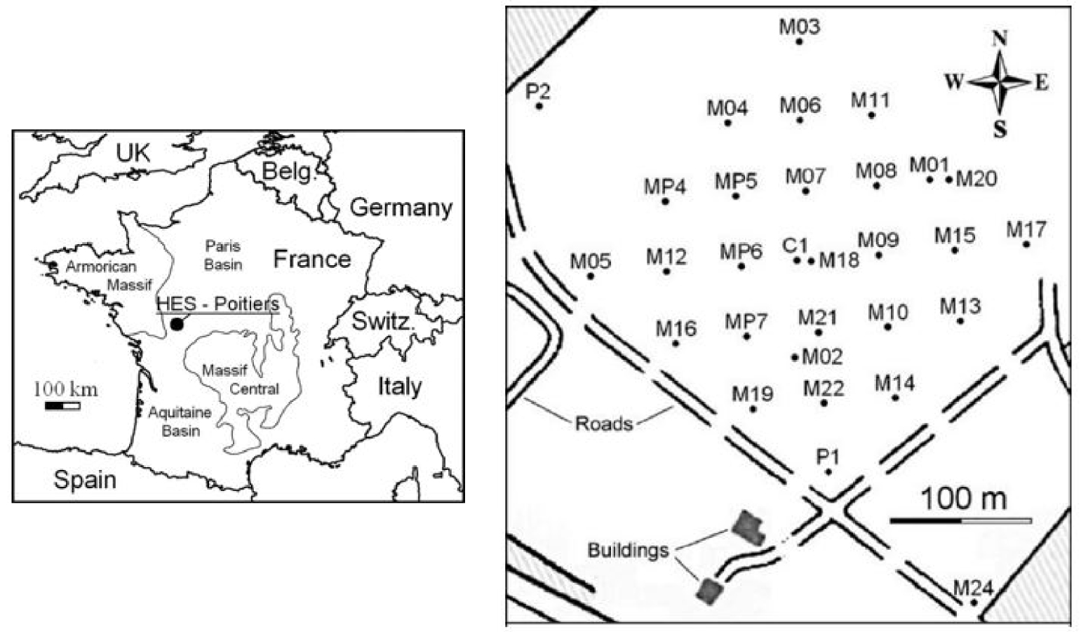
Today, the aquifer responds evenly to the hydraulic stress of a pumped well, with pressure depletion curves (interferences) merged in time and amplitude irrespective of the distance from the pumped well [Ackerer and Delay 2010; Delay et al. 2011; Trottier et al. 2014]. This merging is likely to be a consequence of a local karstic flow developed in open conduits that have been unclogged and connected by the drilling and pumping works. The presence of pervasive karstic drains is supported by logs in the wells using optic imaging. Almost all the wells have shown caves and conduits crosscut by wellbores, with mean apertures of 0.2–0.5 m. These conduits are mostly concealed in three thin horizontal layers at depths of approximately 35, 85, and 110 m. As these open layers are intercepted by almost all vertical wells, this results in a good connection between wells and karstic drains, and eventually between the open layers. The connection would be mainly controlled by the degree to which drains are re-opened in the vicinity of the wells and the connection of drains within a layer.

With the above considerations in mind, it was found reasonable to better image the geometry of the reservoir with a resolution compatible with, on the one hand, the scale of a well and, on the other hand, the scale of the entire experimental disposal. High resolution geophysical tools seem well suited to undertake that kind of investigation.

3. Seismic imaging

The seismic reflection method is able to produce a picture of the subsurface in three dimensions (3-D) over a regular grid. Usually, in high-resolution seismic surveys, the size of the elementary parallelepiped grid cell is of the order of a few tens of meters along the horizontal directions, and of a few (3–5) m along the vertical direction, with an even precision up to 200 m depth. This level of spatial resolution requires dealing with large amounts of raw data and heavy computations for data processing.

At the HES, which is not very large (approximately 300 × 300 × 150 m³), the 3-D seismic survey was refined but designed to obtain a 3-D block recorded in low amounts of data [Mari and Porel 2008]. The complete survey is composed of 20 receiver lines (the in-line direction) with a 15 m lag distance between adjacent lines (Figure 2a), each line being composed of 48 single geophones with 5 m spacing between adjacent geophones. For each receiver line investigated, direct and reverse shots with sources in line with the receiver line were recorded. Cross-line shots fired at distances of 40, 50, and 60 m perpendicular to the receiver line were also recorded (example of cross-line shot in Figure 2b). Processing the data from in-line direct and reverse shots gathers the results in a vertical section of 240 m in-line extension (the blue arrow, in Figure 2a), while a cross-line shot gathers results in a vertical section of only 120 m extension along the in-line direction (the red arrow on the location map of seismic lines, in Figure 2a).

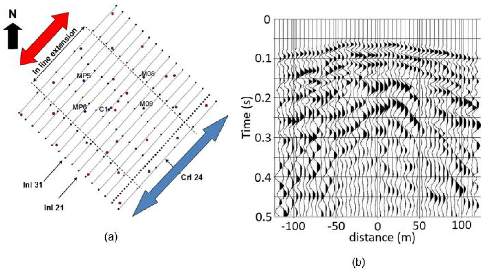
The whole set of single-fold vertical sections of arrival times were assembled to build a 3-D block of 240 and 300 m extension along the in-line and cross-line directions, respectively. For the in-line direction profile, the reference zero in the horizontal direction is taken as the location of the sources points, in the middle of the receiver lines. This renders reflecting point locations varying between −120 and +120 m and a lag distance between two neighbor reflecting points of 2.5 m (half the distance between two adjacent receivers). For the cross-line shots, the reference zero is still taken at the middle of the receiver lines, but with a lag distance between neighbor reflecting points of 5 m.

Seismic data processing was carried out to transform raw arrival times into a 3-D block of wave amplitudes reflected at diverse depth and horizontal locations of the aquifer system. A VSP recorded via geophones placed in well C1 (Figure 3a), was also processed to obtain a law (a conversion) of reflected time versus depth and a velocity model (V_rms) of reflected wave propagation. A 3-D refraction seismic tomography [Mari and Mendes 2012] was finally carried out, with the idea of mapping the irregular shape of the clay cover at the surface (up to 25–30 m depth) overlying the limestone aquifer. This experiment is assumed to render static corrections for the seismic reflected block and a propagation velocity model in the clay cover of the aquifer (also for corrections of the seismic 3-D block).

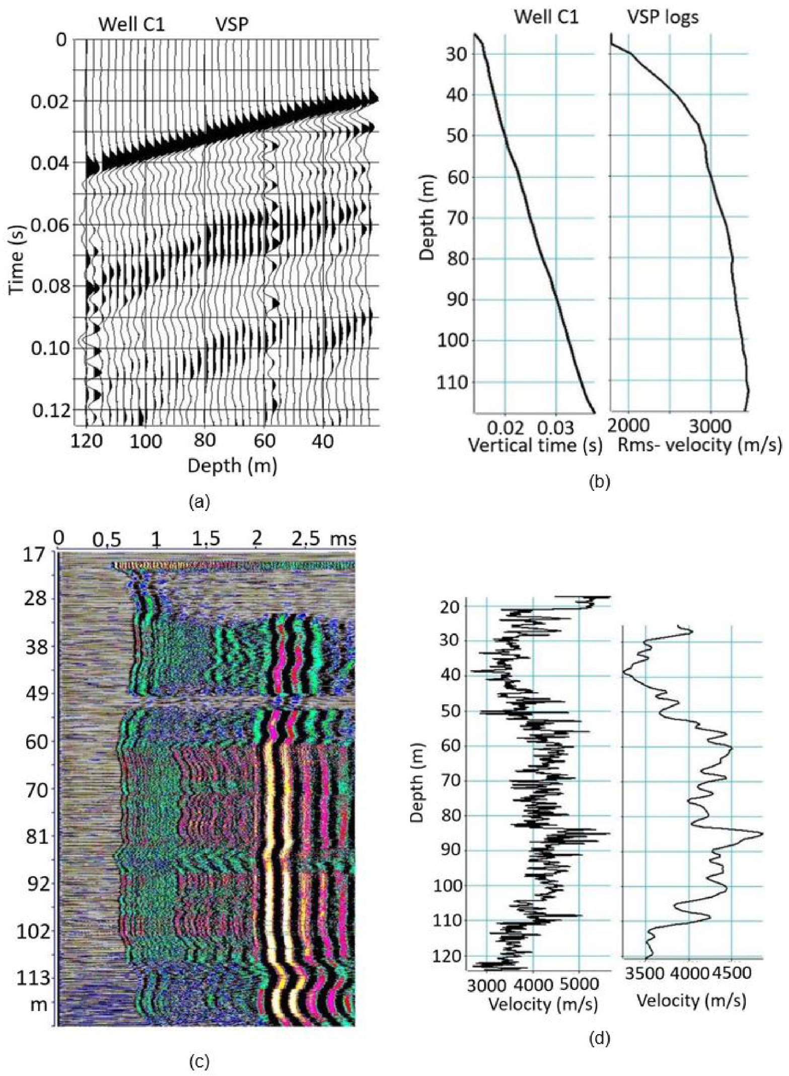
The processing sequence [Mari and Delay 2011; Mari and Porel 2008] includes: amplitude recovery, deconvolution, wave separation, static corrections, and normal move-out corrections (using the VSP velocity model, Figure 3b). Times of the reflected sections were also converted into depths via the VSP time versus depth law inferred in well C1 (Figure 3b).

Acoustic data were also recorded in the boreholes of the HES and that of the well C1 is exemplified hereafter. The acoustic probe is a flexible monopole tool holding a source as a magnetostrictive transducer and two pairs of receivers beneath: a pair of near receivers (1 and 1.25 m lag-distances (offsets) beneath the source) and a pair of far receivers (3 and 3.25 m offsets). The acoustic data were recorded in the 1–20 kHz frequency band. It is worth noting that compared with seismic data, the vertical resolution of the acoustic logging is very high, on the order of 10 cm, but the lateral investigation is limited to a few tens of centimeters around the borehole. Figure 3c reports on the 3 m constant offset section (receiver R1) with the vertical axis as the depth of receiver R1 from ground level, and the horizontal axis the recorded travel times (ms) of acoustic waves from source to receiver. In the acoustic section, the refracted P-waves appear in the 0.5–1.0 ms time window. Sampling the arrival times of the refracted P-wave recorded by two adjacent receivers (R1: 3 m offset, and R2: 3.25 m) allows for obtaining by difference the acoustic velocity within the formation at different depths (Figure 3d). This velocity log is usually highly variable over very short distances, but can be filtered in wavenumber and resampled over larger intervals (here 0.5 m) than the sampling step of the probe (Figure 3d-right). These larger resampling intervals are assumed to be compatible with the vertical resolution of the seismic block, with the aim to constrain the block via acoustic logs. More precisely, the filtered velocity functions computed from acoustic data recorded at wells C1, MP5, MP6, M08, and M09 (locations in Figure 1) were used to convert the 3-D block of seismic wave amplitudes into a 3-D pseudo velocity block [Mari and Delay 2011; Mari and Porel 2008].

It is reiterated that we are interested in evaluating the porosity variations within the aquifer at the HES, under the expectation that high porosity values could mark the locations of karstic features. To this end, the seismic velocities were first converted into electrical resistivity values [Mari et al. 2009], using borehole resistivity logs as calibration and the empirical relationship between seismic velocity and actual formation resistivity proposed by Faust [1953]. This transformation is justified by the fact that we do not have redundant information in terms of velocity propagation because only a few shots were performed over the seismic line implementation at the surface. The velocities are therefore unbounded and may vary from one shot to the other. In the absence of petrophysical data informing on the actual values of velocity propagation over diverse samples of host rocks, the raw velocity data should be calibrated. This is why we relied upon a transformation of velocity into electrical resistivity, according to the empirical non-linear Faust’s law and the 35 logs of resistivity monitored in the wells of the HES. The parameters of the Faust’s law at the wells were interpolated over the whole surface area of the HES and velocities were transformed accordingly into a single 3-D block of electrical resistivity values. Those were then converted into pseudo-porosity values, by using the non-linear Archie’s law [Archie 1942] under the assumption of uniform water resistivity over the whole 3-D block. Figure 4 exemplifies the pseudo velocity and porosity spatial distributions via the in-line #21 section (Figure 4a) and the cross-line #24 section (Figure 4b). A few discrepancies can be observed between the patterns revealed by velocities and those of the transformation into porosities. This is mainly the consequence of the non-linearity of both Faust’s and Archie’s laws in the transformation velocity → resistivity → porosity, and to some extent, an artifact due to color scales in Figure 4 with porosity spanning a larger range of relative values than the velocities. Nevertheless, the images are consistent from one another with areas of weak porosities corresponding to high velocities and high porosity values located in low velocity areas.

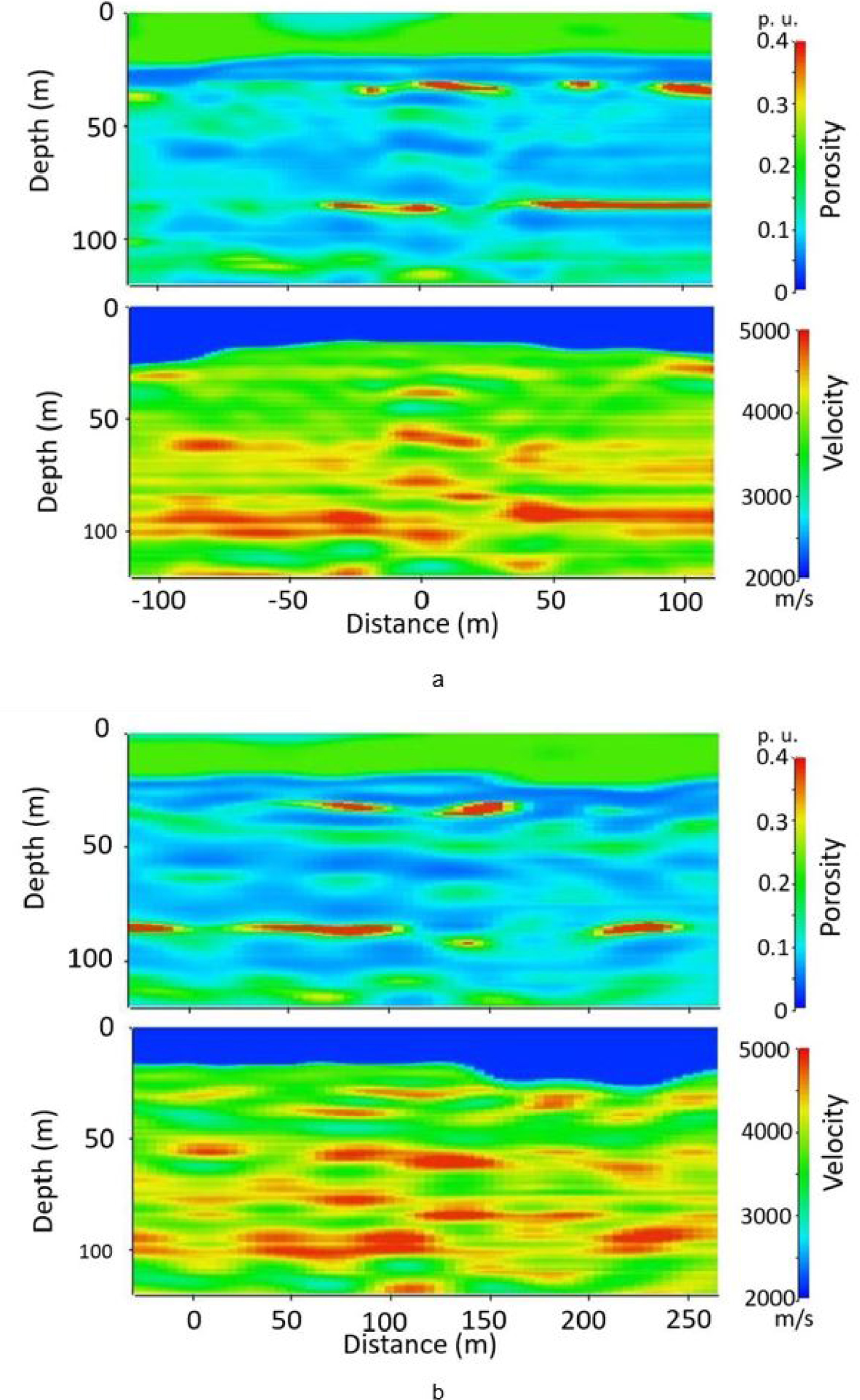
After transformation of the whole set of vertical sections and reassembly, the resulting 3-D seismic pseudo-porosity block (Figure 5) revealed three high-porosity, presumably water-productive layers, at depths of 35–40, 85–87 and 110–115 m [Mari et al. 2020]. The 85–87 m depth layer appears the most porous one, with wide patches of porosity values higher than 30%, that would represent, for this layer, the karstic part of the reservoir (see bottom draw in Figure 5, upper layer).

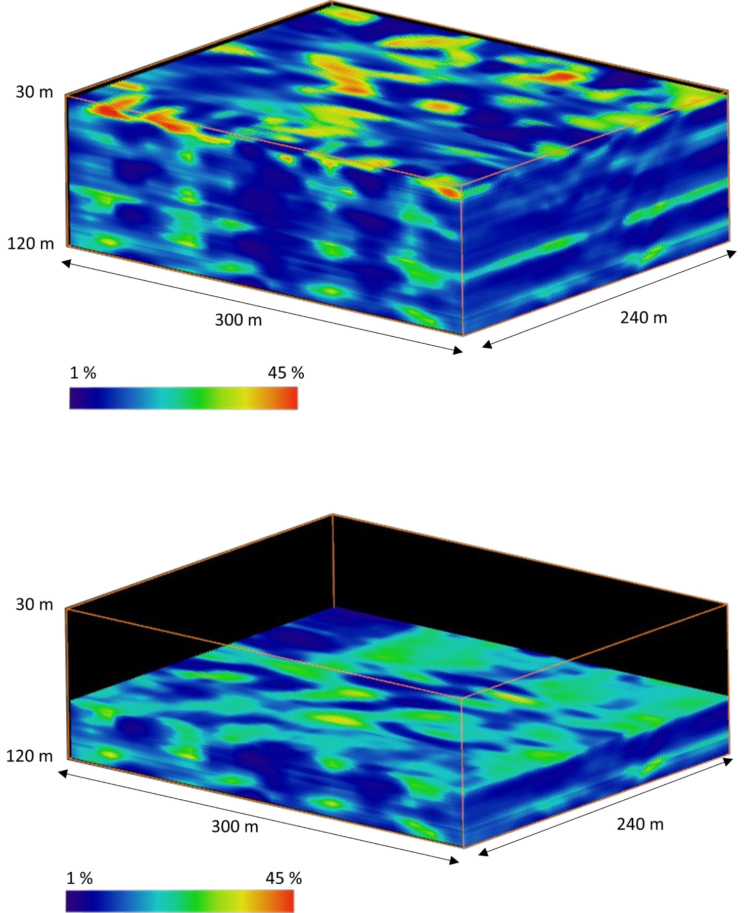
4. Additional information from full waveform acoustic logging

As told earlier, acoustic logging is of very high resolution over depth but investigates a radius of a few tens of centimeters around the well. Full waveform acoustic logging (FWAL) not only analyzes the refracted P-waves propagating in the rock formation crosscut by the well, but also exploits the other acoustic wave lengths monitored by the receivers. After data processing, a FWAL can either confirm or question locally the results from the 3-D seismic block, but also detect small open bodies in the host rock that the seismic resolution is unable to capture. As an example, the acoustic logging in well C1 (Figure 3c) is re-handled for a complete treatment.

The well C1 is equipped with a steel casing from the surface up to 22 m depth, below which, it becomes an open-hole wellbore in which the water table was detected at 20 m depth during the logging. On the acoustic section (Figure 3c), the refracted P-waves appear in the 0.5–1.0 ms time interval, the converted refracted S-waves and pseudo-Rayleigh waves in the 1.2–2 ms time interval, and the Stoneley wave in the 2–3 ms time interval. The logging distinguishes:

• The water table at 20 m depth (no acoustic signal monitored above 20 m), and between 20 and 22 m, some resonances due to a loose cementation of the casing.
• The 22–33 m depth interval with a very poor signal to noise ratio; only refracted P-wave are captured.
• The 33–60 m depth interval with visible refracted P-waves, converted refracted S-waves, and Stoneley waves; in the 49–54 m depth interval, all these waves are strongly attenuated.
• The 60–108 m depth interval of homogeneous profile with a very good signal to noise ratio; all the acoustic waves are visible and of strong amplitude.
• Finally, the 108–124 m depth interval, also relatively homogeneous with refracted P-waves and Stoneley waves of good amplitude; converted refracted S-waves are visible, but noisy.

The acoustic data have been processed in the 35–124 m depth interval, by first picking the arrival times of a wave train to obtain the velocity and the attenuation of the considered wave train [Mari and Vergniault 2018]. Figure 6 shows the results obtained from the refracted P-waves. A log of correlation between signals monitored by the receivers R1 and R2 of the acoustic probe at diverse depths is associated with the velocity log. A high value of the correlation coefficient indicates that the shape of the acoustic signal is the same on the two receivers (R1 and R2). It also indicates that the picked times are accurate. A decrease in the correlation coefficient can sign a poor picking due to either a poor signal to noise ratio, or a change in the signal shape. The correlation coefficient log can be used to “edit” the velocity log, or at least being confident (or not) in some local velocity values (Figure 6a). The wave attenuation log (Figure 6b), calculated for a vertical wave propagation over 0.25 m, is simply defined as the ratio of energy logs at equivalent locations between the log at 3 m offset (distance emitter–receiver R1) and the log at 3.25 m offset (receiver R2). This attenuation expressed in dB/m, is significant at 3 levels located at 50–54 m, 85–90 m, and 110–120 m depth. The two deepest levels are that of the karstic layers revealed by the 3-D seismic imaging. In the 50–54 m depth interval, a low energy, and a very strong attenuation of more than 60 dB/m are observed, even though no karstic (highly porous) layer is detected by the seismic approach.

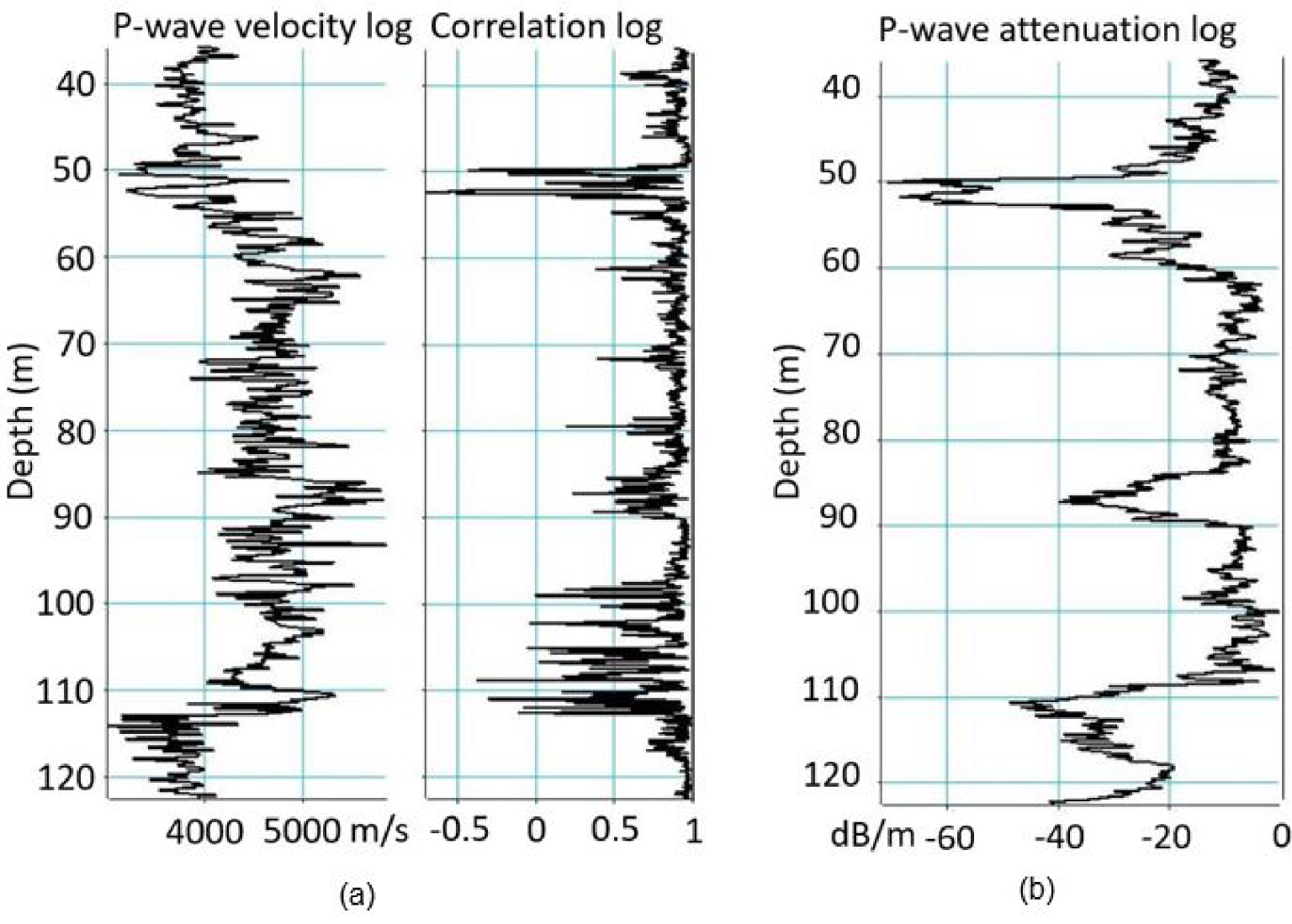
The same procedure has been applied to the Stoneley waves (Figure 7), with energy and attenuation logs of the Stoneley wave underlining the same three levels identified by the analysis of the refracted P-wave. Interestingly, a very strong attenuation is measured in the 50–54 m depth interval, when the attenuation measured in the two deepest levels (85–90 and 110–120 m) is weaker. The energies of the different wave packets depend on the permeability of the ways through which the waves propagate, that are mainly the host rock for P-waves, and the interface between casing and wellbore for Stoneley waves. The sensitivity to changes in permeability is partly evidenced by a loss of total energy in the acoustic signal. The karstic level at 55 m depth crosscut by C1 is confirmed by VSP data recorded using hydrophones (Figure 7c). The VSP is highly corrupted by Stoneley waves. A conversion of downgoing P-wave (blue line in Figure 7c) in down (red line) and up going Stoneley waves is often observed in highly permeable formations [Hardage 1984; Mari and Vergniault 2018; Mari et al. 2020]. In the present case, the first arrivals in the form of downgoing P-waves are strongly attenuated at 55 m, the waves being converted into downgoing Stoneley waves then reflected at the bottom of the well.

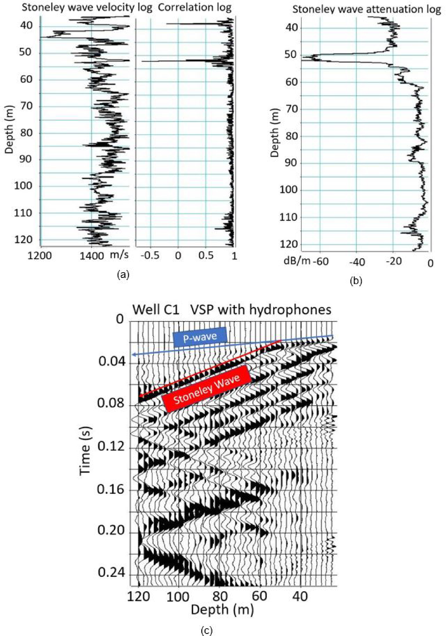
The analysis of acoustic data leads to the following observations:

• The attenuation of the different wave packets indicates that the two deep levels (85–90 m and 110–115 m) revealed by seismic data have a high permeability. This notwithstanding, the continuity of the acoustic images suggests that no geological discontinuity, such as a karstic body, occurring at these depths in the close vicinity of well C1. This interpretation is confirmed by the 3-D seismic block showing that C1 does not crosscut karstic bodies in the 60–120 m depth interval.
• The loss of continuity of acoustic images between 50 and 54 m depth, and the very strong attenuation of the different waves, mainly the Stoneley waves, suggest that this level could be a karstic body with a very small lateral extension at C1 not visible by seismic data.

5. Hydraulic investigations

5.1. Slug tests

In view of the spatial distribution revealed by the seismic 3-D block regarding supposedly highly permeable bodies (Figure 5), the 35 wells regularly disposed at the HES should show variable connections between pairs of wells. It was first proceeded with a series of slugs testing individually each well, but also monitoring the response at distant wells [Audouin and Bodin 2007, 2008]. In its classical form, a slug test investigates a very little portion of the aquifer by injecting instantaneously a small quantity of water (on the order of 100 liters) in the casing of a well [e.g., Butler 2019; Butler et al. 2005; Chen 2006]. Head in the well suddenly increases and its level is monitored over time in the injected well until returning back to the initial state. Usually, the hydraulic stress generated by the injection is not strong enough to observe head responses at distant wells. In the case of highly permeable systems such as the HES, responses to slugs were also monitored at distant wells, which indicated non-negligible head variations (more than 10 cm) up to distances of 100 m. These responses allow for calculating an equivalent (homogeneous) hydraulic diffusion coefficient for 2-D radial horizontal flow between the pairs of injected and monitored wells [Audouin and Bodin 2008]. This coefficient, as the ratio of transmissivity [L²⋅T⁻¹] to storage capacity [−], roughly measures the level of connection between wells for pressure head propagation, but not necessarily water transfer.

Results in terms of hydraulic diffusion between wells are reported in Figure 8. There can exist high contrasts of diffusivity between different close pairs of wells, or between a single well and its neighbors. The size of an elementary five spot in Figure 8a (four wells at the corners of a square, one well at the center) is 75 m, with a few wells 50 m apart from the tested well not responding to the slug tests (e.g., wells MP6, M18, M09, M15, along a W–E line in the middle of the HES) occasionally, or conversely highly connected wells with diffusion coefficients above 10⁵ m²∕s over distances up to 150 m (e.g., pairs of wells M22–M13, M13–M20, M07–M20).

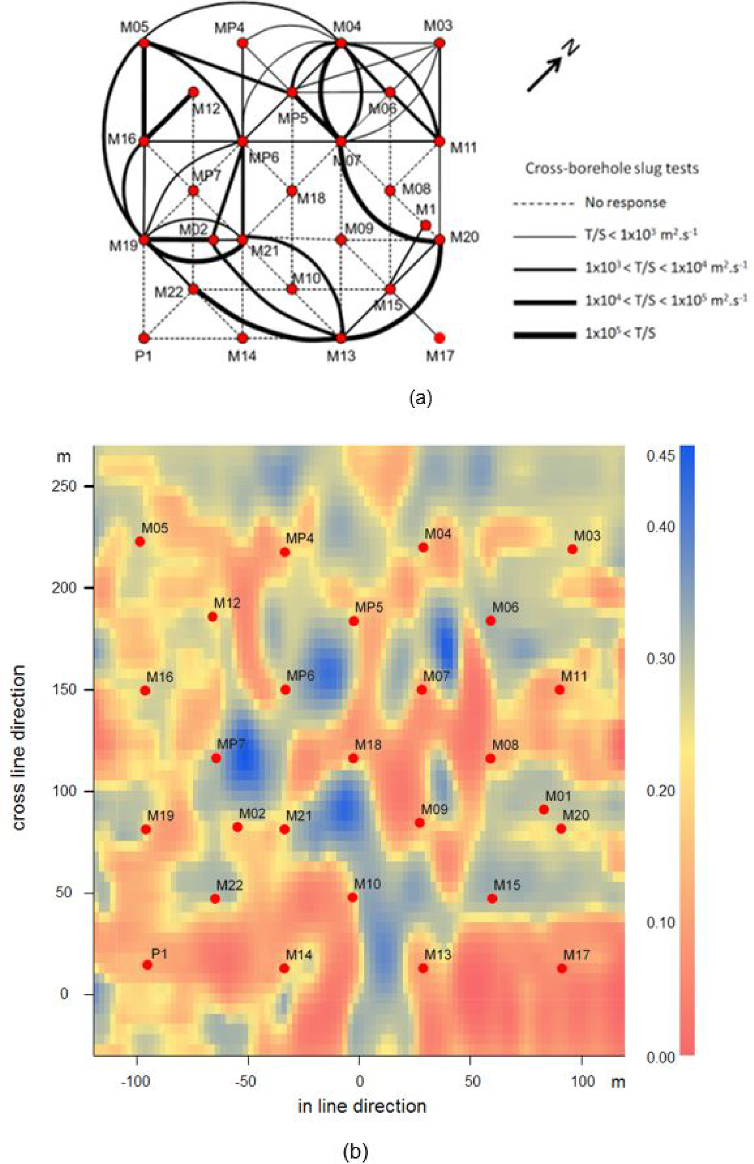
It is not easy to compare the map of connections (diffusivity) between wells and a seismic porosity map, for example the layer at 85–87 m depth extracted from the 3-D block (Figure 8b). At least, the distribution of hydraulic diffusivities between wells is compatible with the overall spreading of high versus low seismic porosity values, showing widespread patches of high-porosity bodies but discontinuous within the layer 85–87 m. This distribution may render pairs of wells located in the same highly porous body (e.g., wells M16, M12), resulting in high hydraulic diffusion for the pairs. Conversely, wells, even close, can be located in non-porous areas (e.g., wells M07, M09), or in separate and non-connected porous areas (e.g., M02, M21), resulting in poor to fair diffusivity values.

It is worth noting that almost all the 35 wells in the HES are open or screened boreholes, fully penetrating the whole thickness of the aquifer, thus providing “artificial” but active connections between the 3 main porous layers evidenced by seismic data. In addition, the limestone host rock is also riddled with vertical fractures of large extension, also prone to connect naturally the 3 porous layers. Both, natural and artificial connections between the layers cannot be evidenced by seismic data, their spatial resolution being not fine enough. Connections between porous layers add complexity to the interpretation of high versus low diffusivity values, because a pair of wells can be not connected to the same porous body within a given layer, but connected within another layer or via boreholes or fractures bridging two different layers (e.g., wells M04, M07 both in separate non porous bodies at 85–87 m but connected elsewhere).

5.3. Inversion of spatially distributed subsurface flow

As told earlier, with a set of interference testing covering the whole HES, and resulting in evenly distributed information (transient drawdowns), an inversion of flow at the scale of the HES can be attempted, with the aim to identify the distribution of hydraulic parameters resulting in flow simulations similar to drawdown observations. Head or drawdown observations in open wellbores usually do not see the vertical components of flow, because head values are homogenized in the wellbore and are almost uniform over its whole depth. This feature does not prohibit carrying out an inversion of flow over a three-dimensional system. But with lack of conditioning data, the distribution of hydraulic parameters, especially along the vertical direction should be highly conjectured.

Two main attempts of inverting interference testing assuming two-dimensional flow and aimed at retrieving the spatial distribution of hydraulic parameters were carried out. One attempt relied upon a forward flow model in a dual-porosity medium. By assuming that both a fractured medium and a matrix medium coexist at the same location everywhere in the system, the approach is prone to homogenize the seismic structural heterogeneity seemingly separating diverse subareas between highly-porous (flowing) patterns versus weakly-porous (non-flowing) entities. The results from the inversion of a dual-porosity aquifer (not reported here) rendered bimodal (fracture) hydraulic conductivities at either 10⁻³ or 10⁻⁵ m∕s, but distributed over the whole HES as wide patches of almost uniform values [Trottier et al. 2014].

The other attempt employed a forward two-dimensional flow model in a single-porosity medium. It was assumed that a single medium with contrasted hydraulic properties could render valuable flow simulations of interference testing. The resulting parameter fields should also mark contrasted regions of hydraulic behavior, as revealed by the structural seismic images. Flow in a single porosity medium is probably a slightly flawed hypothesis for grounding in the forward problem, because we already mentioned that flow was probably not fully diffusive in a confined system (see above). This notwithstanding, by selecting a large number of data (5597 transient head values spread over the whole HES) and a parsimonious parameterization, eventual slight misconceptions in the forward model are expected not to render results worse than those associated with measurement errors on heads.

With the idea of regrouping all available flow information in a single package conditioning inversion, six interference testing were regrouped into a fictitious scenario adding sequentially over time the drawdown responses at distant wells. A relaxation period was added between the periods pumping in a single well, allowing for the water table to come back to its initial value. Raw data of drawdowns were resampled with a logarithmic time step to avoid giving more weight to short pumping times. The whole history of resampled drawdowns was introduced in a simple least-square objective function adding the squared errors on heads between simulations and observations. No regularization terms were added to the objective function, the aim being of letting the inverse problem and flow data to seek the appropriate parameter values and spatial distributions without any prior guess on them.

Parameterization for both specific storage capacity and hydraulic conductivity employed the so-called adaptive multiscale parameterization [AMT, Ackerer and Delay 2010; Ackerer et al. 2014]. The principle is to superimpose over the (forward problem) computation grid, a coarse triangular mesh, also referred to as the parameter grid. The nodes of the parameter grid hold a few local parameter values serving as seeds in any type of smooth interpolation calculating the effective parameter value in each cell (element) of the computation grid. The seed parameters are those manipulated by the optimization technique seeking the best inverse solution. During the optimization, the parameter grid can be refined locally, which also states that increasing locally the number of seeds may help to improve the depiction of parameter heterogeneity for better inverse solutions [Ackerer et al. 2014]. Local refinements obey two main criteria on either the local value of errors between model outputs and data (i.e. the local value of the objective function), or the gradient components (with respect to parameters) of the objective function. With almost zero value local errors between model outputs and data, needless to refine locally the parameter grid. Conversely, important errors would incline to refine the grid. Regarding the local components of the objective function, a stiff local gradient component indicates that the grid can be refined, when a flat component tells that the inverse problem is locally not sensitive and does not deserve further parameter grid refinement. It is worth noting that this overall parametrization procedure is let free of retrieving any spatial distribution of parameters, notably that witnessed by flow data only.

With a few refinements of the parameter grid, the number of seeds, that is, the number of master parameters sought by the inversion, may rapidly reach a few hundreds. In the present context, with almost 5600 data values, the problem is not over-parameterized. The parameterization is also easily manipulated by the optimization technique relying upon a Quasi-Newton method supplemented by the calculation of a discrete adjoint state to flow [Ackerer et al. 2014] to infer the gradient components of the objective function.

As an example, Figure 9a reports on the observed and simulated drawdown curves at a few monitored wells in the sequential flowing scenario. Simulations fit fairly well the observations. Over 50 equiprobable inverse solutions were calculated (by randomizing the AMT parameterization procedure), any error on head never exceeded a few centimeters for drawdowns values between 1 and 5 m. Figure 9b is an example of inverse solution as the map of hydraulic conductivities retrieved at the scale of the computation grid. The scale of the map is not that of the seismic block and encloses a wider area surrounding the zone of interest with all the wells of the HES. This surrounding shows that the AMT parameterization technique rapidly stops its grid refinements over areas with lack of data, thus rendering almost uniform values of parameters. Here, conductivity values around the area of interest are relatively small, on the order of 10⁻⁷–10⁻⁸ m∕s, as a good way to “naturally” avoid noise propagated by boundary conditions (even if those are far from the HES).

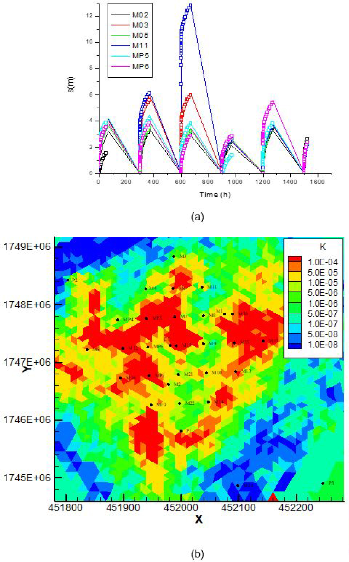
5.4. Hydraulic conductivities compared with structural heterogeneity

Glancing at the hydraulic conductivity map in Figure 9b shows that the hydraulic heterogeneity revealed by inverting flow is not the structural heterogeneity revealed by seismic data. Straight at the HES, the conductivities vary between 10⁻⁴ and 10⁻⁶ m∕s. They are distributed as large patches of convoluted contours with high conductivity to the NW and the SE of the site separated by a central area (N–S line between wells M11 and M22) of low values. For the purpose of easier comparison with the structural heterogeneity of the seismic block, a 2-D map of seismic porosity is draw as the averaged porosity values along the vertical direction of the three porous layers encountered at 35–40, 85–87 and 110–115 m depth (Figure 10). This map is that of a high porosity layer (values between 0.15 and 0.3) uniformly bombed with low porosity (0.05) patches of 20–50 m extension. The high porosity layer, presumably highly conductive, is still continuous, and connected over the HES but populated with many small islands of weakly-conductive formations. In any case, the image rendered by the seismic porosity is not that from flow inversions as a system highly conductive over its largest part with a single weakly-conductive band in its central part.

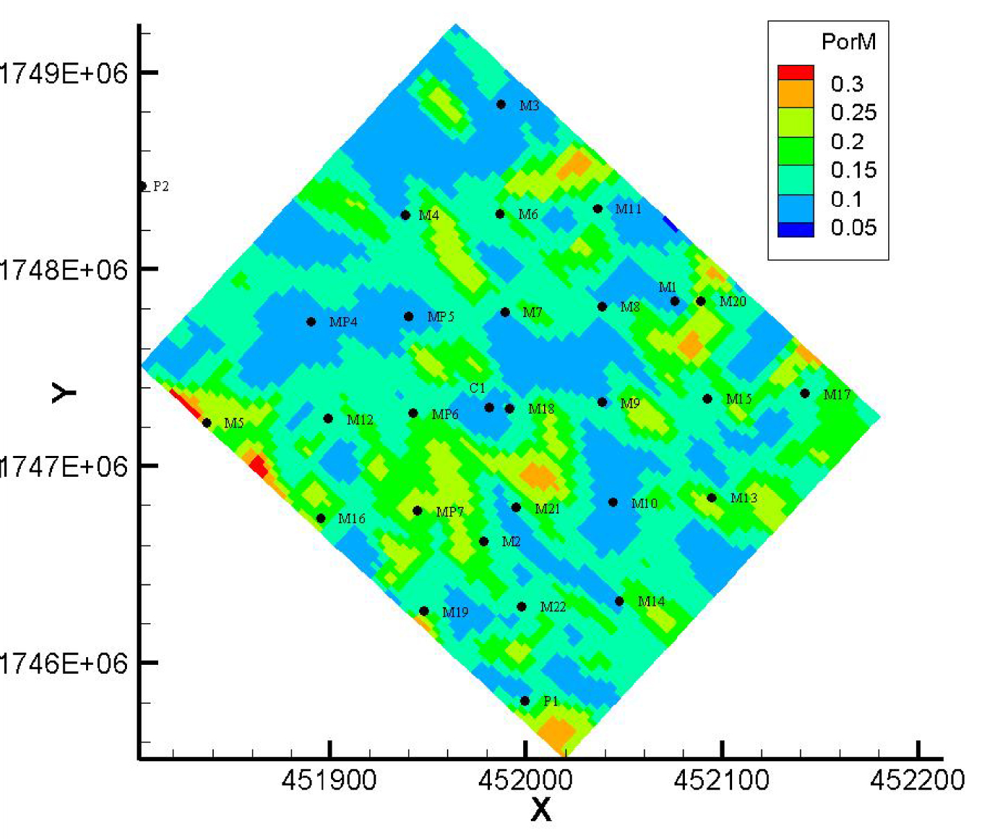
Therefore, it must be concluded that seismic data, even collected at a scale compatible with that of flow computations (and hydraulic parameters), evidence a structural information which is not the hydraulic heterogeneity stemming from flow pattern inversion. Several reasons to this embarrassing question can be mentioned.

• Flow is usually considered as a process robust to its parameters with the meaning that hydraulic parameters must be varied over wide ranges to observe significant modifications in flow patterns. This often yields in inversion exercises to relatively smooth parameter fields with large correlation lengths [e.g., Ackerer and Delay 2010; Trottier et al. 2014]. For their part, seismic data, and especially wave velocities in porous formations, are highly sensitive to bulk rock densities variations over short distances.
• As mentioned earlier, seismic data are not sensitive, given their spatial resolution, to smaller features, as the loose network of vertical fractures riddling the subsurface at the HES, or the network of 35 open wellbores enhancing hydraulic connection between the diverse layers of the HES. Fractures and open wellbores are witnesses by flow as rapid pathways, if these features are hydraulically active (not clogged).
• Seismic data, and also acoustic logs, have been geared towards detecting karstic bodies. But their detection does not predict if those bodies are fully open to flow or partly clogged by infilling materials such as sandy clay. Several works at the HES did not deny the existence of karstic bodies in a few layers of the HES. But it was mentioned that these bodies could have been initially clogged and partly reopened, especially close to the wellbores by drilling works and hydraulic investigations [e.g., Kaczmaryk and Delay 2007b; Audouin and Bodin 2008; Ackerer and Delay 2010]. The partial re-opening changed the overall hydraulic behavior of the HES, increasing connectivity between wells and ensuring rapid propagation of head variations within the subsurface. With seismic data hardly making the difference between clogged and open karstic bodies, it is not illogical that the structural heterogeneity evidenced by seismics is not the effective hydraulic heterogeneity.
• As an aside, which also goes with the preceding observation, regarding connections; the HES today probably has a too dense network of wells. Within its building phase, it was ignored that the wells would crosscut layers of very contrasted hydraulic behavior. Thus, the site was designed for highly resolved hydraulic experiments and mass transfer experiments at the field scale, but carried out over reasonable durations. With 35 wells connecting highly conductive layers, it is very likely that interference testing and other hydraulic tests are partly corrupted by a rapid propagation of pressure head variations via pipes. This also applies to the 2-D modeling of flow as that used for inversions. Some prospective simulations of 3-D flow, explicitly accounting for wells as conductive pipes, could probably tell us to which extent, the excess of connection by vertical wells corrupts the assumption of a large-scale two-dimensional flow.

However, a question remains unanswered. The structural heterogeneity from seismics has not been inverted regarding groundwater flow. It is well documented in the ongoing literature that the inverse problem if often ill-posed, a consequence being here that multiple solutions exist with sometimes very different patterns. It can be wondered on how the structural heterogeneity could reproduce interference testing at the HES. The seismic block could be segmented into a few classes of porosity values; those classes being each assigned a specific “facies” with its own hydraulic parameters. This would result into a small number of parameters distributed over a 3-D block, then inverted by modifying the parameter values without changing their spatial distribution. This task is still to be undertaken but takes a form out of the scope of the present work. Several options could be selected for the purpose of comparisons. For example: (1) a 3-D approach to Darcian flow in a single porosity system with at least an explicit representation of preferential flow along the wells, and inverting flow data only, or flow data and a pre-conditioning of parameters onto the seismic structure; (2) the same approach in terms of data and pre-conditioning of inversion but with dual-porosity systems or local inertial effects on Darcian flow (to account for preferential flow and eventual lack of Lorentz reciprocity).

6. Conclusions

We exemplified how near subsurface geophysics can be employed to image the structural heterogeneity of a karstified limestone aquifer. This aquifer is not a karst in the typical sense mainly composed of caves, open conduits etc. It is a standard porous and fractured limestone, concealing a continuous confined ground water system, but with the sparse occurrence of open karstic bodies that mainly appear along three partly dissolved layers of 2–5 m thickness at 35, 85 and 110 m depth. This type of structure is not straightforward to detect only via vertical wells. The reason is that karstic bodies are of small aperture (0.5 m) and not continuous over each layer. Therefore, a wellbore can either crosscut an open feature or miss it, but in any case, the well does not inform on the lateral extension of the open body and its eventual connection with others.

High resolution seismic data reveal an interesting technique to image open bodies in the near subsurface, as the local wave propagation velocities are sensitive to the density of rocks, in short, their small versus large porosity. The technique is also non-intrusive, with all the investigations carried out from the surface, even if a few wells are welcome to obtain a reference (a model) of wave velocity over depth. Seismic data can be complemented by acoustic logs and vertical seismic profiles along wells; they mainly detect very small open bodies close to wells and not identified by seismic data.

3-D seismic data, eventually coupled with logs, is probably not a suitable combination to image karstic aquifers at the regional scale, to fix the ideas, over territories of several km of horizontal extension. But as shown in this study, the resulting images are of sufficient resolution for the accurate delineation of fractured or karstic bodies at a scale compatible with the security perimeter usually surrounding subsurface catchments for water supply. In view of the short transit times associated with preferential flow paths in karstified aquifers, and the subsequent risks of rapid contamination of catchments, it makes sense to envision 3-D seismic as a valuable tool for assessing the effectiveness of such perimeters.

Unfortunately, in the specific case of the HES, the structural heterogeneity revealed by 3-D seismic data is not that revealed by inversion of flow on the basis of high resolution hydraulic data from interference testing. Hydraulic heterogeneity here is of much wider correlation length separating large zones of high conduction neighboring large zones weakly connected. For its part, the 3-D seismic proposes a highly conductive field simply populated with small clusters of non-conductive areas. With the idea suggested above that karstified systems need for the assessment of mass transfer characteristics, both types of heterogeneity would not render the same flow patterns and, by the way, very different transport scenarios.

It is not completely clear why these divergences between hydraulic and structural images exist. But is worth noting that the HES has been completely remodeled by important drilling works and hydraulic tests under forced flow conditions. Those could have changed the diverse connections between layers in the aquifer or within the same layer, things that are not captured by seismic data.

A duplication of high resolution geophysics imaging to other hydrological contexts would be welcome. As mentioned earlier, the HES is probably plagued by an excess of connections due to the number of wells and the reopening of porous bodies by drilling works and hydraulic investigations. For example, if the delineation of an experimental site was foreseen, a prior analysis via geophysics imaging, which could also include electrical resistivity tomography (ERT) and magnetic resonance sounding (MRS) could be attempted. A second campaign of the same measurements after finalization of the diverse facilities at the site could tell us how geophysical imaging and incidentally the hydraulic behavior are sensitive to our “invasive” fingerprint in the system.

This study posed the question of how near subsurface geophysics could help groundwater flow inversion. The answer is that geophysics at the very least reveals new ideas on the subsurface heterogeneity and should motivate hydrogeologists to widen their conceptual models (families) of inverse solutions. In 1999, G. de Marsily et al. published a paper on “Forty years of inverse problems in Hydrogeology”. More than twenty years later, sixty years of inverse problems let the question open.

Conflicts of interest

Authors have no conflict of interest to declare.