


 CC-BY 4.0
1. Introduction
It is well known since the pioneering work of Dunne [1969, 1980] and Dunne and Black [1970] that saturated groundwater flow (both subsurface and deep) plays an important role in forming and sustaining channelized flow, especially in humid environments. From this perspective, neither can streams be considered as merely fixed (Dirichlet) boundary conditions for the groundwater system, nor can the groundwater flow feeding the streams be considered a mere “baseflow contribution”: the energy level in the aquifer system and in the streams are strongly related for all flow conditions.
Wyns et al. [2004] showed that in low conductivity, shallow aquifer systems (such as weathered crystalline basement settings), there is a strong relation between the groundwater level at a given location, and the drop in topographic elevation from this location to the nearest wet talweg. More precisely, there is a correlation between the height above a basal envelope surface of talwegs (height labeled a on Figure 1), and the height of the groundwater level above this same envelope surface (height labeled b). In such systems, the low hydraulic conductivity implies a steepening of groundwater head gradients in order to convey groundwater from hillslopes to channels.
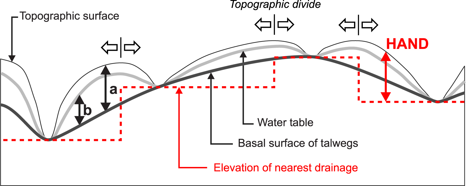
Illustration of different potentiometric levels on a topographic/groundwater transect, adapted from Wyns et al. [2004] in order to show both the Basal Surface of Talwegs and the Elevation of Nearest Drainage of Nobre et al. [2011].
Obviously, the steepest gradients are achieved when the groundwater potentiometric surface is close to the topographic surface, i.e.
Interestingly, a parallel concept has been introduced in the field of flood mapping, namely the Height Above Nearest Drainage (HAND) of Nobre et al. [2011]. There are a couple of differences between the two relative elevations defined respectively by the Height Above the Basal Envelope Surface of Talwegs (HABEST) and the HAND. These differences are illustrated in Figure 1:
- the HAND computation procedure relies on a hydrologically-conditioned Digital Elevation Model (DEM) in which a reference drainage network is identified using a minimum support area. It then requires a downstream drainage allocation of each pixel, so that it creates a jump at the crossing of a water divide when two pixels on either side of the divide are “snapped” to two distinct drainages. Put differently, the reference potentiometric surface from which the HAND is computed is not continuous (we should call it the Elevation of Nearest Drainage, though it is not explicitly introduced by Nobre et al. [2011]).
- In contrast, the surface constructed following Wyns et al. [2004] is continuous. It is produced by interpolating point-scale elevation data in the talweg network.
From the point of view of free surface (channel) flow, a surface of minimum potential energy joining all the talwegs is of course, an important reference level: the transient rise of water during a flood event corresponds to a relative elevation above the “normal” drainage level, i.e. a local HAND value [Nobre et al. 2016].
Since the computation of such a base level has several applications, there is a need to give a formal definition and an unambiguous procedure to compute it.
2. A formal definition of the Basal Envelope Surface of Talwegs (BEST)
Let us consider the vertically-integrated, transient diffusivity equation for groundwater flow with the Dupuit–Forchheimer assumption [e.g., De Marsily 1986]:
| (1) |
| (2) |
Assuming a uniform or slowly-varying transmissivity across the domain, we can take T out of the divergence operator. In the following, we will assume a strictly uniform transmissivity T0, hence:
| (3) |
We can consider a hypothetical situation where the groundwater level reaches a minimum (∂h∕∂t ≈ 0) in conjunction with a vanishing recharge rate (r(x,y,t) ≈ 0), with the perennial streams still connected with the shallow aquifer. The head distribution would then satisfy:
| (4) |
where ztopo denotes the elevation of the topographic surface. Petroff et al. [2012] as well as Cohen et al. [2015] have studied in great detail the interaction of a stream network with a Poisson diffusive field in the more general case of a nonlinear transmissivity T(h) = K ⋅ (h − B) for an unconfined aquifer, where B(x,y) denotes the elevation of the underlying impermeable layer and K the saturated hydraulic conductivity of the aquifer. In the following, we will restrict ourselves to the linear case, as it allows simple analytic developments based on the superposition principle. Here, the condition 𝛥h = 0 means that the flux density
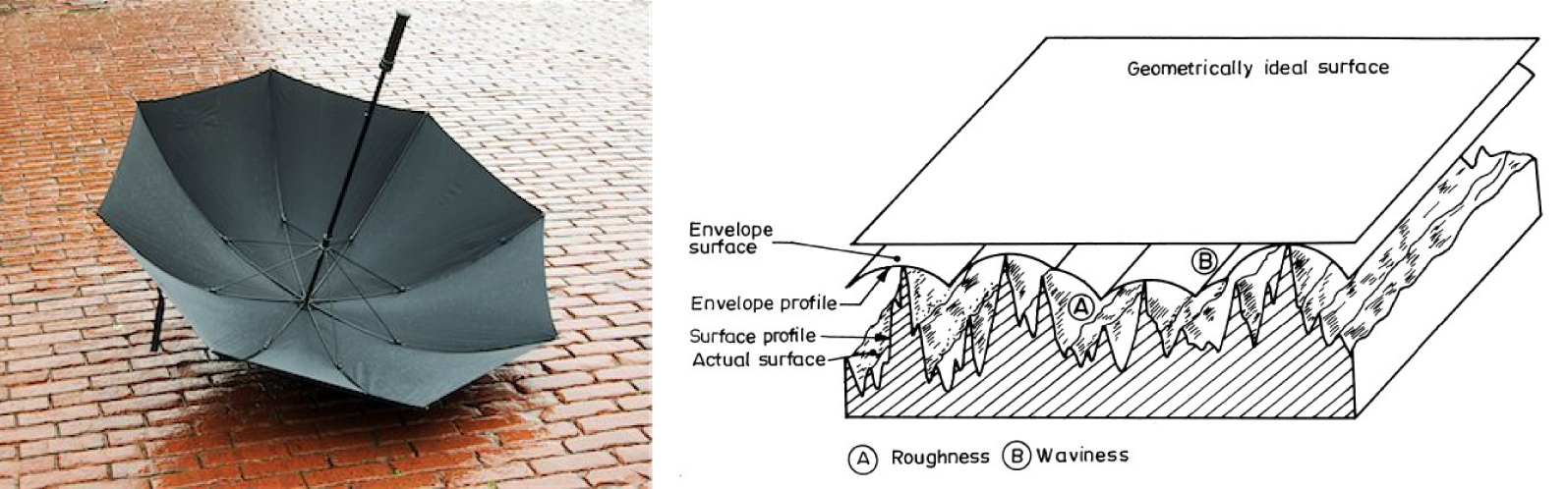
(Left) Example of an envelope surface, in the form of the canopy of an umbrella; (right) definition by Häsing [1964].
Usually [see e.g., Deffontaines 1990; Wyns et al. 2004; Yao et al. 2017], this surface is constructed by kriging of scattered talweg elevation data: a more straightforward way of constructing it is to solve (4). In fact, under the assumption of uniform transmissivity we can directly model the analytic function using the Analytic Element Method [AEM, see e.g. Strack 1989; Steward 2020], instead of solving the steady-state equilibrium equation numerically with stream elevations as Dirichlet boundary conditions. As will be shown further, the procedure boils down to a simple linear least-square optimization, without the need for variography.
3. Mathematical modeling with analytic slit elements
3.1. Vector representation of the talweg graph
The approach proposed in this study relies on a vector representation of the talweg or stream network. Such representations are usually provided by national geographic agencies, as it is the case for the BD Topage in France [Système d’Information sur l’Eau/Sandre 2020], but can also be derived from the analysis of Digital Elevation Models (DEM). The network is a set of links, i.e., sections of a stream channel connecting two successive junctions, a junction and the outlet, or a junction and the drainage divide [ESRI 2022]. We assume that the topology of the links is also available in the form of an oriented graph. This general setting is illustrated in Figure 3. Each link is a polyline that can be decomposed into segments, each defined by a start point Aj and an end point Bj.
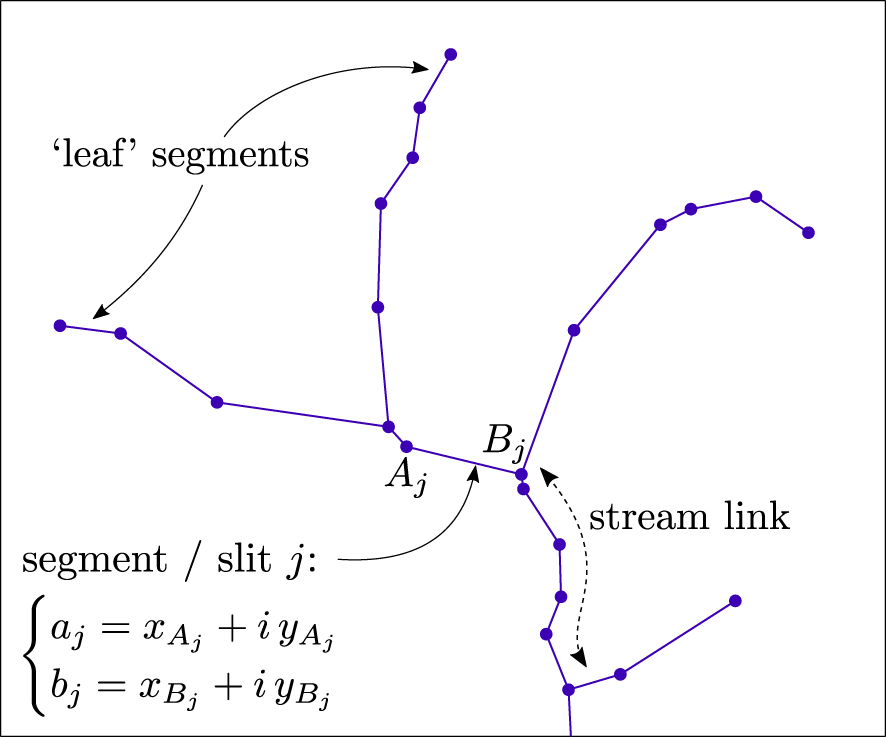
Vector representation of the talweg or stream network. It is a collection of elementary segments/slits, each defined by two endpoints which can be positioned in the complex
Vector representation of the talweg or stream network. It is a collection of elementary segments/slits, each defined by two endpoints which can be positioned in the complex
3.2. General form of the potential
In AEM, the head distribution is related to a real-valued potential 𝛷 [e.g., De Marsily 1986], such that:
For unconfined aquifers such as the shallow groundwater systems developed in weathered bedrock, our focus in this study, the general form of the flux is:
In the case of a piecewise uniform elevation B of the substratum (i.e.
This expression hence leads to a nonlinear relation between potential 𝛷 (in m3∕s) and head h (in m). In the following, we will linearize the problem and consider a uniform transmissivity T0 of the groundwater system, independent of h. This linearization is motivated by several considerations:
- first, as weathering develops from the surface down, it is no stronger an assumption to consider a rather uniform depth for the lower limit of the transmissive layer, than to consider a piecewise uniform elevation for this limit; this amounts to assume a rather uniform saturated thickness at first order, if the groundwater table is always close to the surface;
- second, our objective is to use observed groundwater levels in boreholes as well as topographic elevation of streams in order to infer large-scale hydrodynamic properties of the system such as, precisely, an “effective”, large-scale estimate of transmissivity. This is much easier to do when using groundwater head h directly as a proxy, linearly related to potential 𝛷: it will be clear when we present the degrees of freedom used to compute the value of potential 𝛷 using AEM in the next paragraphs.
With the assumption of a uniform transmissivity T0, the potential 𝛷 is indeed linearly related to groundwater head h:
| (5) |
| (6) |
with i, a number such that i2 = −1. Hereafter, the letter z will denote an affix z = x + i y in the complex plane (with the exception of ztopo which will denote the topographic elevation). In the case of a divergence-free flux density
Following the approach of Steward [2015, 2020], we will then consider each segment j of the talweg network as a slit element creating a complex potential 𝛺j(z) at location z, with the form:
| (7) |
Qj is the net algebraic discharge (in m3∕s) entering the slit, and the cj,k are the complex coefficients of a Laurent series that can be adjusted to match various boundary conditions. If Qj > 0, the slit is a sink to the system (it subtracts water from the aquifer) while if Qj < 0, it is a source (it leaks water to the aquifer). The mapping function Zj(z) for each slit element is given by:
| (8) |
| (9) |
The function
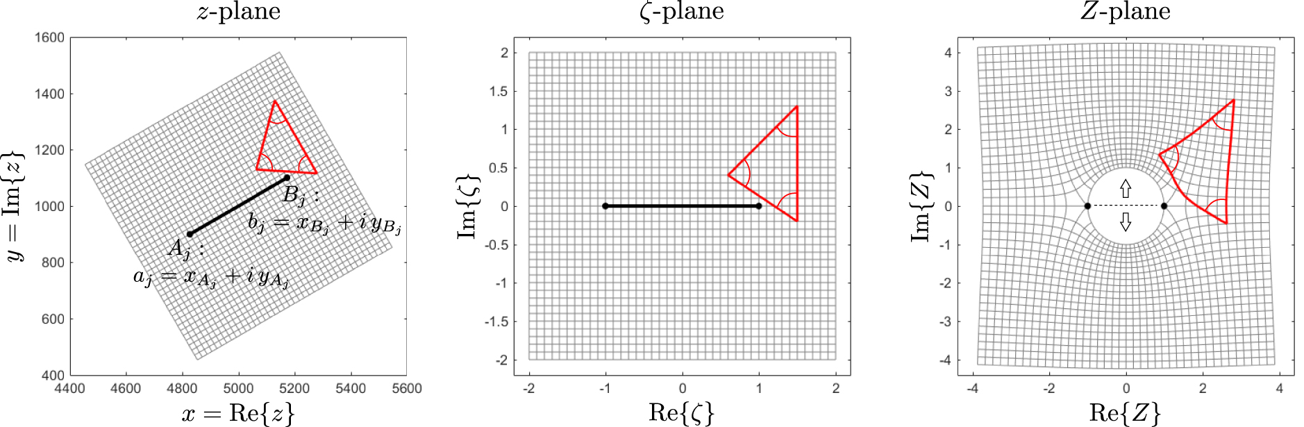
Illustration of the transformation Zj(z) associated to slit element j, with endpoints Aj and Bj. It is obtained by the composition of a similarity 𝜁j(z), and the Joukowsky transformation
Illustration of the transformation Zj(z) associated to slit element j, with endpoints Aj and Bj. It is obtained by the composition of a similarity 𝜁j(z), and the Joukowsky transformation Lire la suite
By superposition, the total (complex) potential at location z in the complex plane is simply the sum of the contributions of all slit elements in the domain:
| (10) |
For each element j, we have (2nc + 1) real degrees of freedom: the sink term Qj, the nc real parts Re{cj,k} and nc imaginary parts Im{cj,k} with cj,k = Re{cj,k} + i Im{cj,k}. Together with 𝛷0, v0,x, and v0,y, the total number of real degrees of freedom is thus N = 3 + ns × (2nc + 1).
In Figure 5 we show the general form of the potential for three cases:
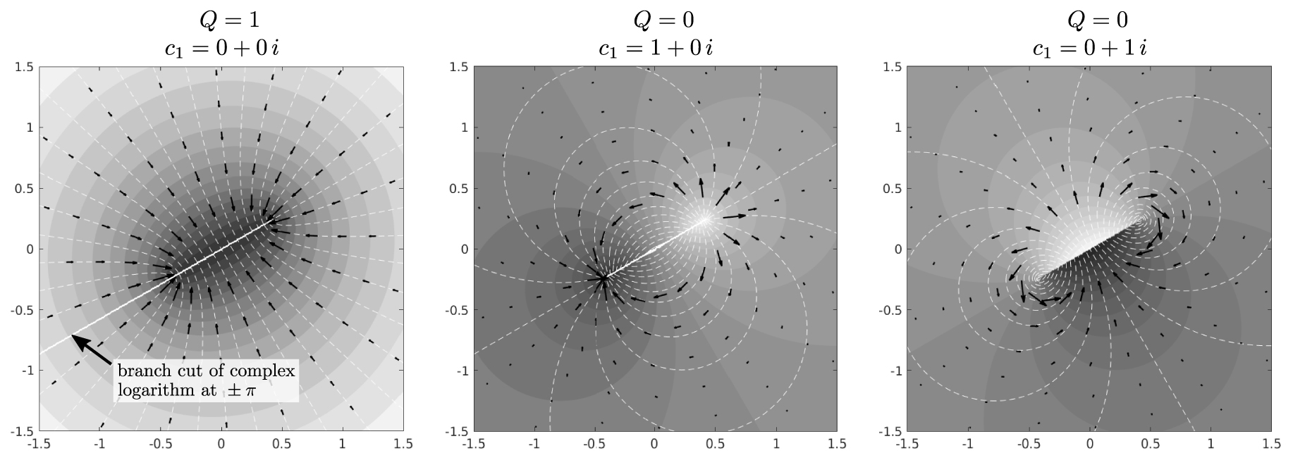
General form of the potential created by a slit element. In each figure, the gray levels show the value of 𝛷 = Re{𝛺(z)} while the dashed white lines are contours of the stream function 𝛹 = Im{𝛺(z)}. Black arrows show the flux vector
General form of the potential created by a slit element. In each figure, the gray levels show the value of 𝛷 = Re{𝛺(z)} while the dashed white lines are contours of the stream function 𝛹 = Im{𝛺(z)}. Black ... Lire la suite
- a pure sink element with Q≠0 and all terms set to zero in the Laurent series; far from the slit, the real potential created by such an element is identical to the well known Thiem solution h = 𝛷∕T0 = (Q∕2πT0)lnr + constant [e.g., De Marsily 1986],
- the potential 𝛺(z) = c1 Z−1(z) with a real-valued c1 coefficient. In this case, the real potential 𝛷 (gray levels) is continuous,
- the potential 𝛺(z) = c1 Z−1(z) with a pure imaginary c1 coefficient. In this case, the real potential 𝛷 is discontinuous across the slit.
The two last situations do no produce any net inflow nor outflow.
Of course, in the general case we have no idea of the transmissivity of the porous medium; in order to work directly with head levels/drops we will normalize the expression of the complex potential by the (unknown) uniform transmissivity T0:
| (11) |
3.3. Optimization procedure
Given a set of control points {zp}1⩽p⩽M where we want to specify a value
| (12) |
The control points are positioned along the segments of the stream network. Since there are 2nc + 1 degrees of freedom for each slit, the system is overdetermined if we position more control points than this value along each segment. The vector of optimum values for the parameters (the 𝛽l’s) is the least squares solution to:
Instead of Dirichlet conditions at control points, we can also specify Neumann conditions on the normalized velocity vector
Using the chain rule
This expression is again linear with respect to all real degrees of freedom.
4. Two applications of the Basal Envelope Surface of Talwegs
4.1. Study site: the Evel catchment and Coët-Dan subcatchment
We illustrate the concepts of the previous section on a small catchment located in Brittany (Western France), the Coët-Dan catchment, where surveys have been conducted since the early 1970s [Fovet et al. 2018]. This catchment is developed on brioverian shale with low hydraulic conductivity. In order to avoid edge effect, we consider the larger catchment of the Upper Evel River in which the Coët-Dan catchment is completely nested (gauging site J5618322—Evel at Remungol).
4.1.1. Digital elevation model and derived vector datasets
Figure 6 shows the map of topographic elevation. The original data is the 1-m resolution RGE ALTI [Institut Géographique National 2018]; in order to speed up the extraction of the hydrographic network without altering channel elevations, we downscale this dataset to a resolution of 5 m by keeping the minimum elevation on each 5 × 5 pixels block. The resulting DEM is then hydrologically conditioned, and the flow direction and flow accumulation maps are computed. The stream network is extracted in vector form from the DEM with a support area of 0.1 km2 [ESRI 2022]. The boundary of the Evel catchment is also extracted in vector form, as the segments making up this boundary will be assigned a zero normal velocity condition in the least squares regression. In order to reduce the geometrical complexity, the stream links and the boundary polyline are simplified using the Douglas–Peucker algorithm [Douglas and Peucker 1973] with a planar tolerance of 40 m.
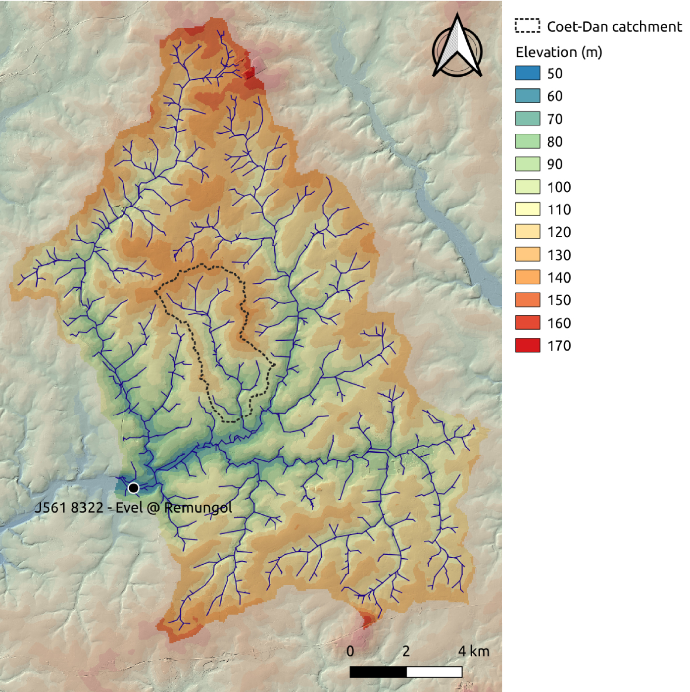
Map of the Upper Evel catchment and the nested Coët-Dan subcatchment. The vector stream network is extracted with a support area of 0.1 km2.
4.1.2. Estimation of the Basal Envelope Surface of Talwegs
The total number of segments in the geometric setting is given in Table 1, along with the associated degrees of freedom.
List of the degrees of freedom in the least squares problem
| Type of elements | Number of elements | Number of sink terms |
Number of |
Number of |
Number of degrees of freedom |
|---|---|---|---|---|---|
| Stream segm. | 1562 | 0 | 2 × 1562 | 0 | 3124 |
| Boundary segm. | 176 | 0 | 2 × 176 | 2 × 176 | 704 |
| Total incl. |
3829 |
We use ncoef = 2 complex coefficients for the Laurent series on each slit element, that is, up to 4 real degrees of freedom per slit. However, we recall that in order for the real potential 𝛷 to be continuous between the two “sides” of a slit, the imaginary parts of these coefficients must be zero: hence there are only 2 real degrees of freedom for stream slit elements. This condition of continuity is not required for boundary slit elements: here we only want the normal velocity component to be zero on the “inner” side of each slit. We completely disregard the value of the real potential outside of the boundary, so we use both a real part Re{cj,k} and an imaginary Im{cj,k} part for the 2 complex coefficients of each boundary slit element. We set the background velocity to zero (v0,x = v0,y = 0), but the constant 𝛷0 is needed in any case and yields an additional degree of freedom, rising this number to 3829.
In order to get a least squares solution for all degrees of freedom, we use the overspecification principle of Janković and Barnes [1999] with M = 8 control points on each slit, whose positions are given by:
The total number of control points is then M × nslit = 8 × (1562 + 176) = 13,904, much larger than the number of degrees of freedom (3829). This resulting system is 13,904 × 3829, which is rather large, but still very easily solved by classical linear algebra packages. If we were to solve an even larger system, we could use the iterative solution introduced by Janković and Barnes [1999], sequentially solving for the coefficients of each slit to match its boundary conditions while holding all other coefficients constant for other slits, until convergence is reached [see also, e.g., Steward 2020].
Figure 7 shows the resulting envelope surface, that is, the real part
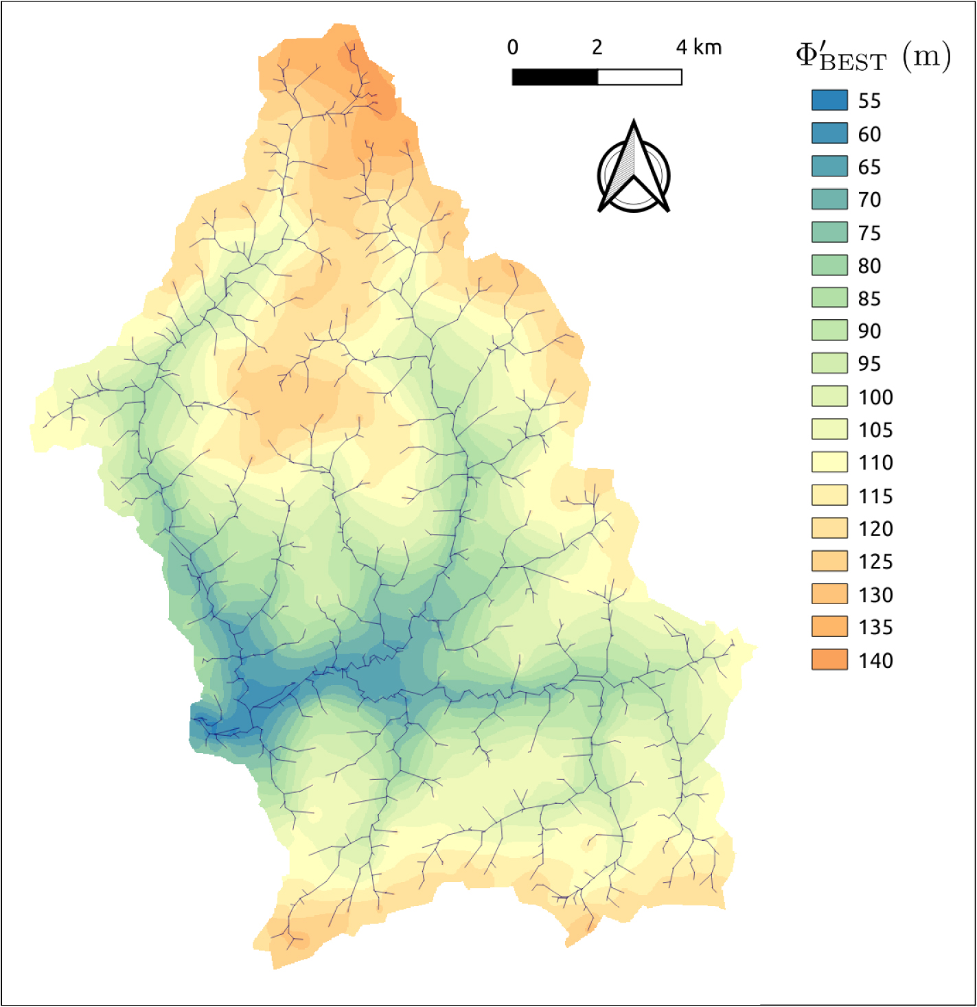
Elevation map of the Basal Envelope Surface of Talwegs (BEST) resulting from the least squares regression against talweg elevations, with a Neumann condition on the boundary.
4.2. HABEST as a continuous substitute of HAND for flood mapping
Having built a continuous energy level joining all talweg lines, we can now compute the difference between the Basal Envelope Surface of Talwegs (BEST) and the topographic surface. This difference can be coined Height Above the Basal Envelope Surface of Talwegs (HABEST). It is conceptually the same thing as the Height Above Nearest Drainage’ (HAND), with two advantages:
- It is continuous in space. The HAND computation procedure requires a downstream drainage allocation of each pixel, so it creates a jump at the crossing of a water divide when two pixels on either side of the divide are “snapped” to two distinct drainages;
- if a reference hydrographic network is available in vector form, there is no need for hydrological preconditioning of the DEM (cf. Section 4.1.1).
Figure 8 shows the resulting index
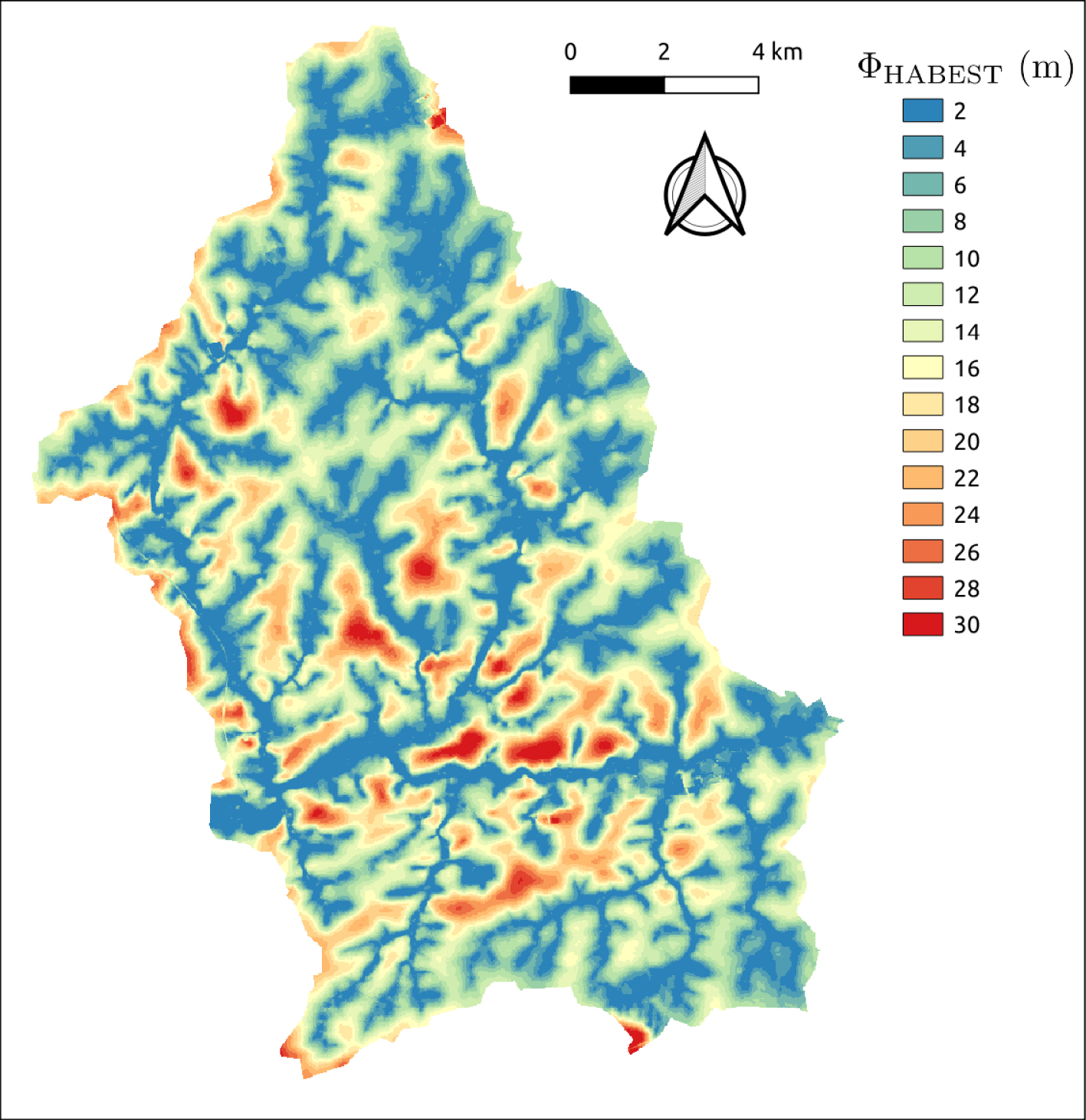
Map of the Height Above the Basal Envelope Surface of Talwegs (HABEST) index, defined as the difference between topographic elevation
Map of the Height Above the Basal Envelope Surface of Talwegs (HABEST) index, defined as the difference between topographic elevation
4.3. Groundwater level interpolation
4.3.1. Regression using HABEST as predictor
In this section, we use the resulting HABEST index as a predictor for groundwater level, following the idea of Wyns et al. [2004]. Figure 9 is a zoom on the map of Figure 7 on the Coët-Dan subcatchment; it also shows the location of 74 boreholes in which the groundwater level was surveyed during the month of February, 1996 [Pauwels et al. 1996]. The model reads:
| (13) |
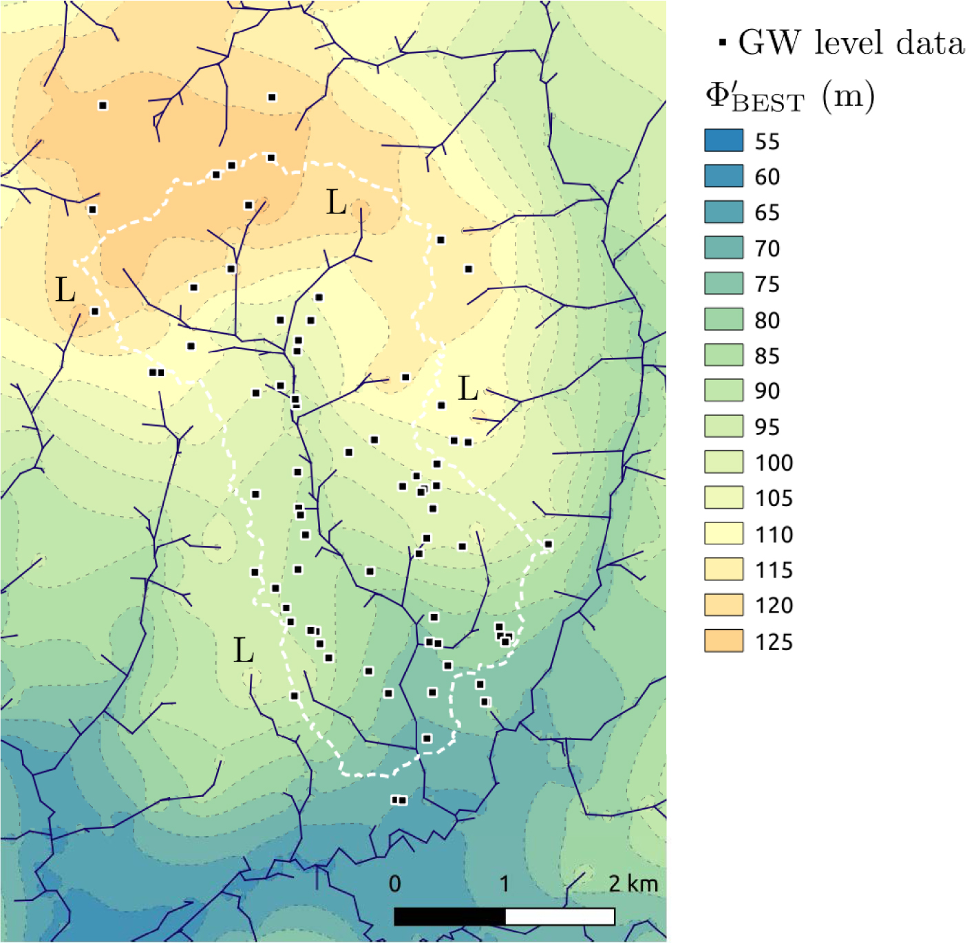
Close-up on the elevation map of the Basal Envelope Surface of Talwegs in the Coët Dan subcatchment (dashed white line). Black squares indicate the location of the 74 boreholes in which the groundwater level was surveyed during the month of February, 1996.
The result of the regression is shown in Figure 10. The parameters are:
Result of the regression of relative groundwater above the Basal Envelope Surface of Talwegs,
Result of the regression of relative groundwater above the Basal Envelope Surface of Talwegs,
It is worth noting that the estimate of groundwater level using (13) is not completely insensitive to the value of the support area chosen for extracting the channel network. The RMSE obtained for different values of the support area is shown in Figure 11; we see that the optimal value is about Ac = 0.4 km2.
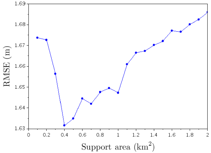
Rooted-Mean-Squared-Error (RMSE) of the regression of
Rooted-Mean-Squared-Error (RMSE) of the regression of
4.3.2. A non-zero divergence solution with area-sink
The definition of the envelope surface as a harmonic potential (corresponding to a divergence-free velocity field) is straightforward, and the result shown in Figure 7 exactly corresponds to the specifications so far. However, if we look closer at Figure 9, we see that slits corresponding to “leaves” in the network graph often correspond to a maximum of the envelope surface, just as if the surface was locally “hanging” from those elements, with the flux oriented from the slit to the domain (see points denoted with a “L”). It is no big issue if we do not want to give any particular physical meaning to this envelope surface; however, this is a spurious behaviour if we want to interpret it, for instance, as a (dry-season) groundwater level.
We can achieve a slightly more satisfactory interpolating surface by computing a non-zero divergence velocity field, still using AEM. For this we will set a non-zero sink term Qj for each stream slit, in conjunction with an area sink [Strack 2017] with uniform infiltration rate. The Laplacian of the potential now satisfies the following steady-state equation away from the slits:
Since we add a source term in the system, we need to add one or several sink term(s) somewhere else: obviously, it has to be at stream slits. The idea is to make the sink term Qj for each slit element j a function of 𝛾0. Let consider the portion of the stream slit graph shown in Figure 12: if we assume that we have only very local flow systems, we can consider that each slit cannot extract more than the amount of recharge on the subcatchment, it drains. Denoting dAj the area of this subcatchment, which is a purely geometric quantity that can be easily computed in a Geographic Information System (GIS), we will even consider that the two quantities exactly match:
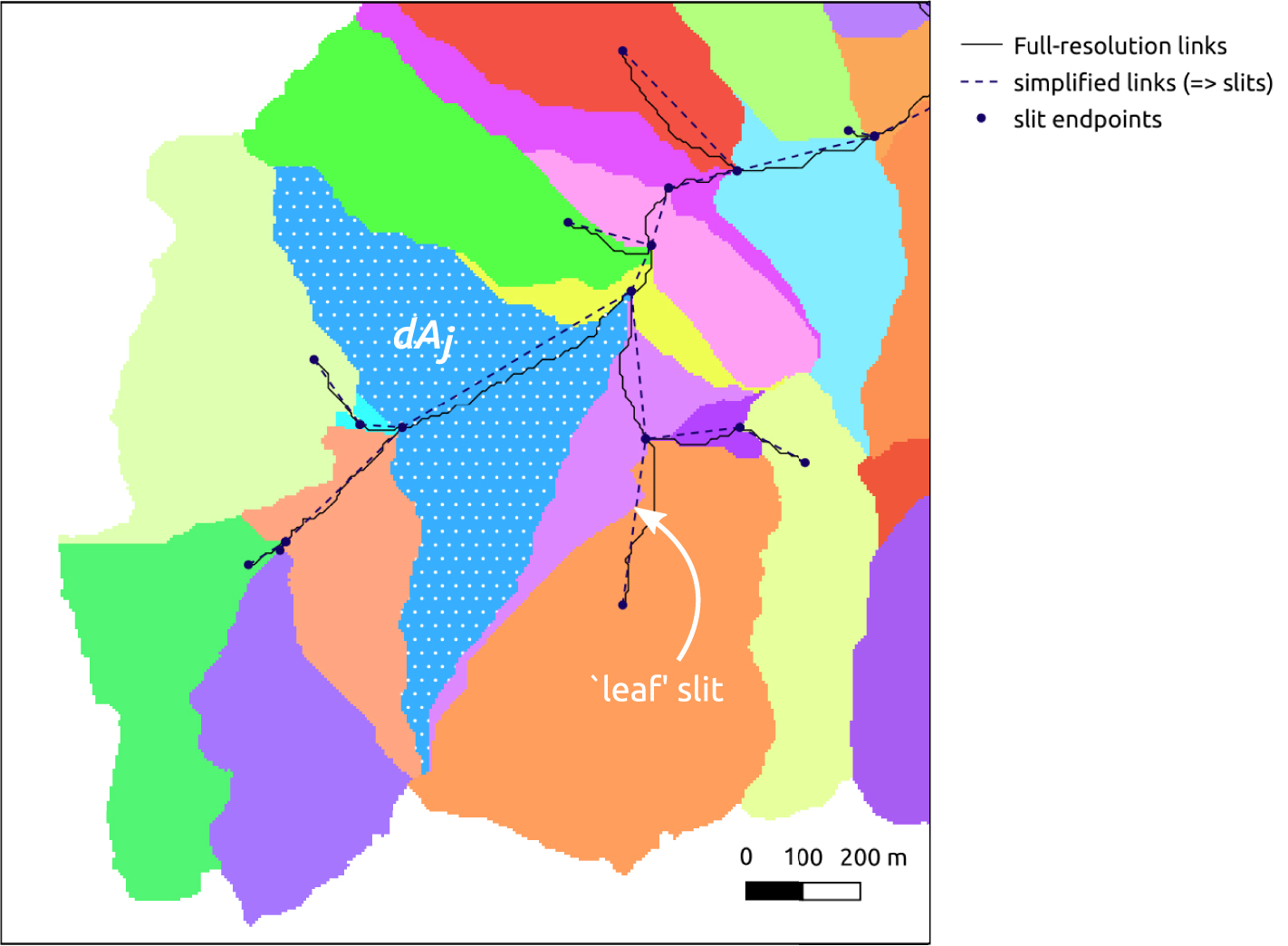
For each stream slit j, we compute dAj the area of the subcatchment drained by the slit, that is, the difference between the value of the flow accumulation map at the downstream endpoint of the slit minus the value at the upstream endpoint. For “leaf” slits, dAj is simply set to the drained areal at the downstream end of the slit. Each slit is then allowed to extract a normalized discharge
For each stream slit j, we compute dAj the area of the subcatchment drained by the slit, that is, the difference between the value of the flow accumulation map at the downstream endpoint of the slit minus ... Lire la suite
It is worth reiterating the fact that even though Qj represents a flux extracted from the groundwater system, it does not necessarily represent a contribution to streamflow. A fraction of this flux might as well represent riparian or wetland evapotranspiration concentrated in the vicinity of the talweg, especially for the smallest streams that often dry up during summertime.
For the sake of brevity, the reader is referred to Strack [2017] for the expression of 𝛷areal(z) and the associated velocity vareal(z). Both are linear with respect to the new degree of freedom 𝛾0. Of course, there is no stream function 𝛹areal associated with 𝛷areal: because of the non-zero divergence there is no holomorphic complex potential. Figure 13 shows the contours of 𝛷areal for a unit extraction rate 𝛾0 = 1.
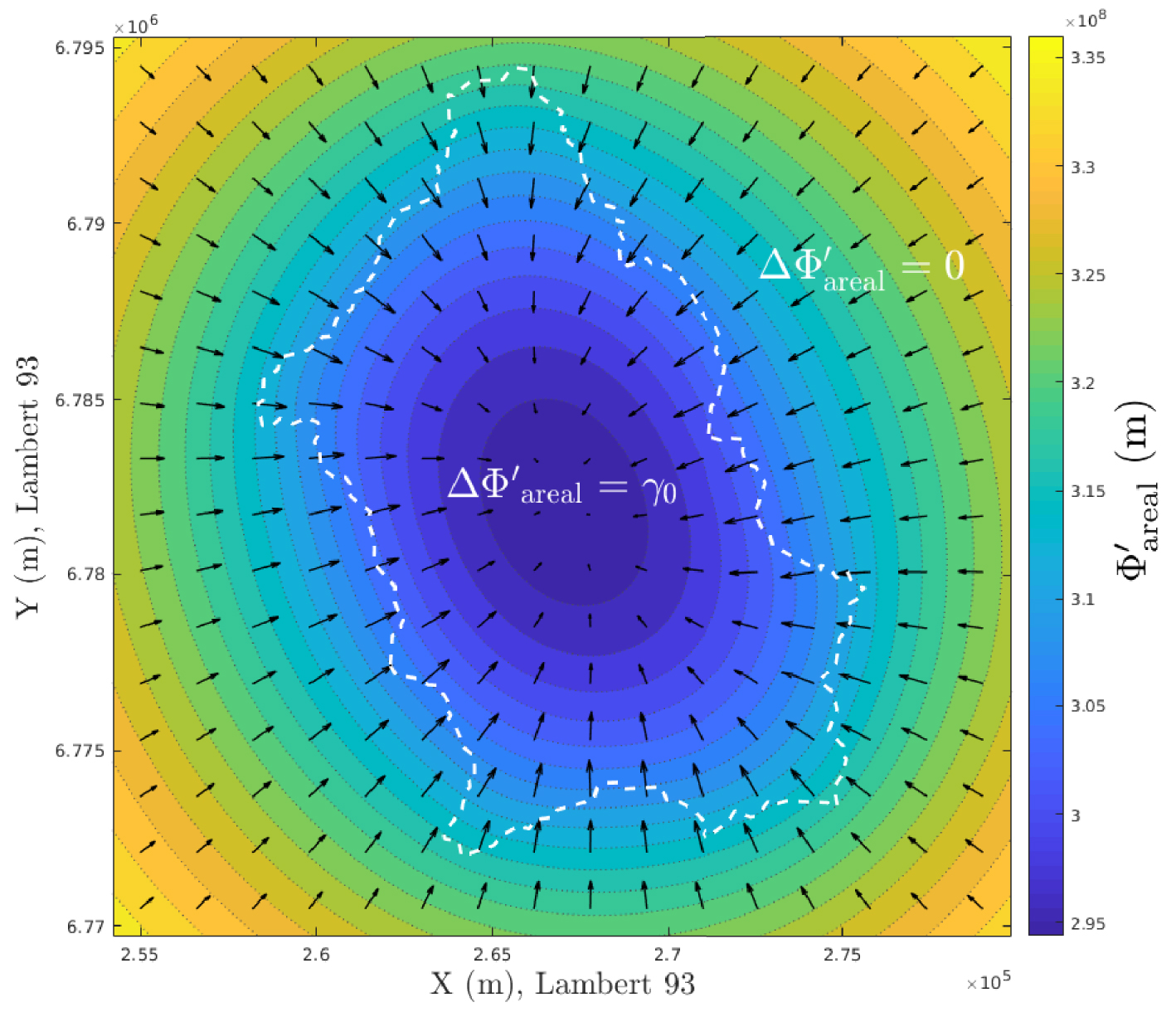
Contour map of real potential created by an areal sink of unit normalized extraction rate 𝛾0 = −r0∕T0 = 1. The Laplacian of the potential uniformly equals 𝛾0 inside the polygon (white dashed line), and it is harmonic outside (
Contour map of real potential created by an areal sink of unit normalized extraction rate 𝛾0 = −r0∕T0 = 1. The Laplacian of the potential uniformly equals 𝛾0 inside the polygon (white dashed line), and it is harmonic ... Lire la suite
By superposition, the real potential produced by all elements in the domain finally reads:
Just as before, the coefficients of the Laurent series cj,k for stream slits are real-valued in order to ensure the continuity of 𝛷′, while the coefficients cj ′,k for boundary slits can remain complex-valued as long as we are not interested in computing a potential outside of the boundary.
The degrees of freedom are better identified with ancillary potential data at groundwater observation boreholes. Figure 14 shows the final map; the regression yields 𝛾0 = −1.19 × 10⁻⁴ m−1.
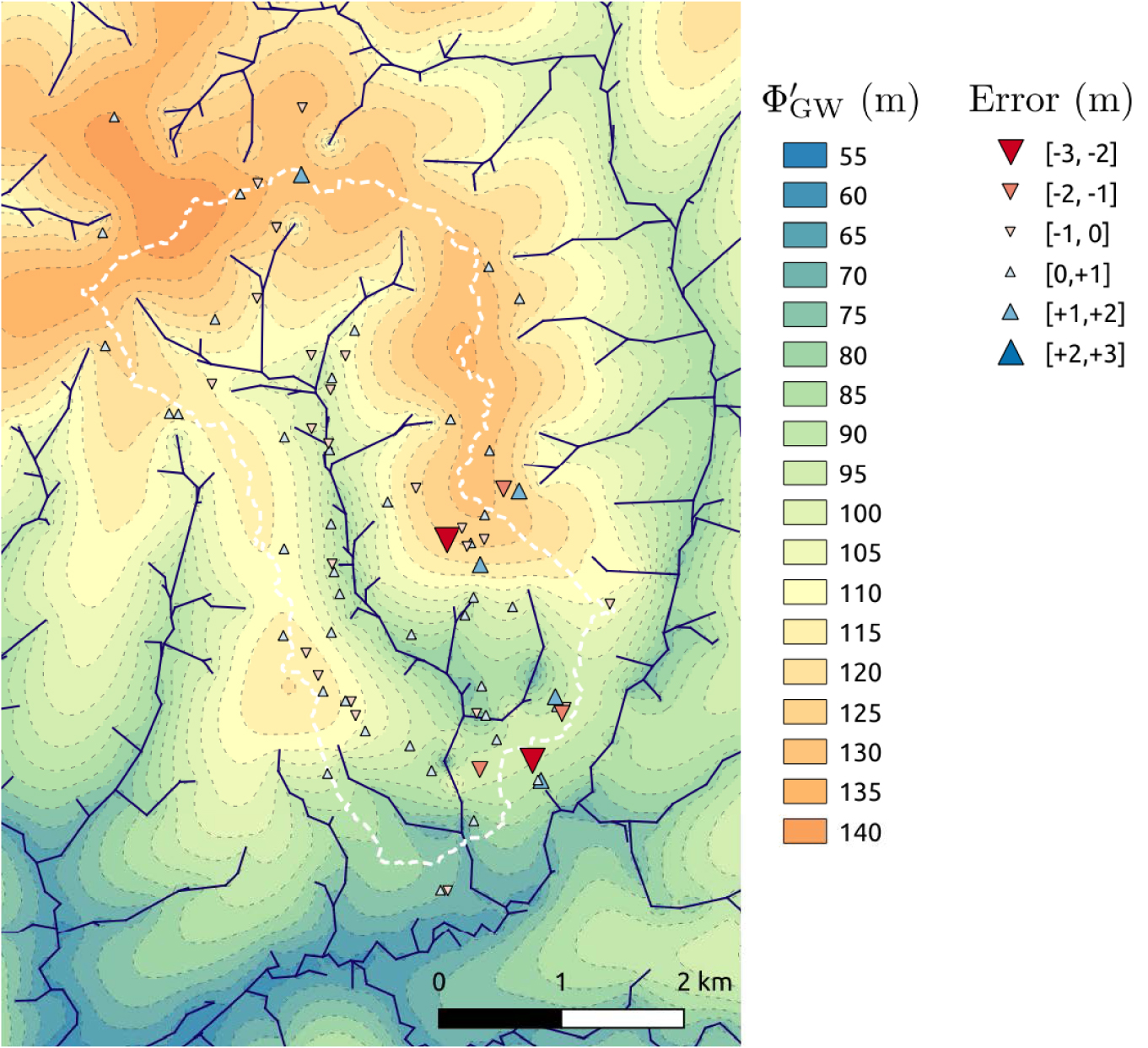
Simulated map of the groundwater potential
Simulated map of the groundwater potential
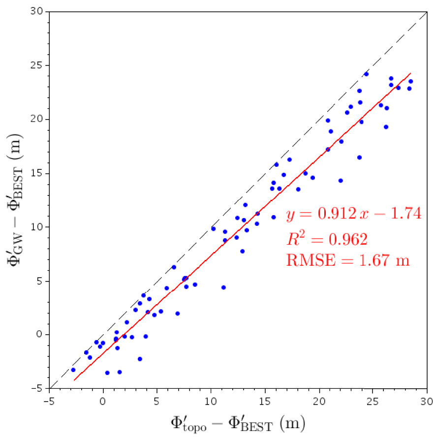
In Figure 15, we compare the observed versus estimated groundwater level at the 74 observation boreholes. In order to narrow down the range of values we plot the estimated depth,
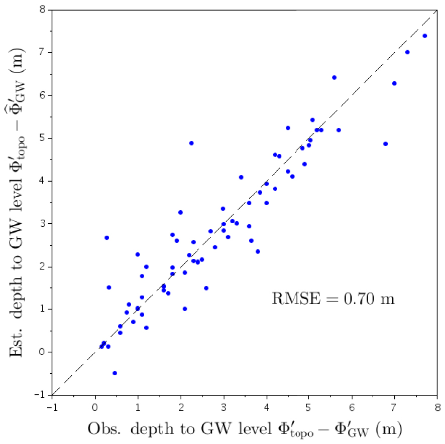
Scatter plot of observed versus estimated depth to groundwater level with the additional degree of freedom 𝛾0 (normalized areal exfiltration rate).
Interestingly, if we have an independent estimate of recharge rate r0, we can get an estimate of large-scale, single-layer equivalent transmissivity. Various estimates of annual effective rainfall can be found in the literature for the region, ranging from 180 mm [Mougin et al. 2004] to 393 mm [BRGM 2019]. Taking a mean estimate and considering a 50%–50% partition of this amount between surface runoff and recharge, this leads to a rough estimate of r0 ≃ 4.5 × 10⁻⁹ m⋅s−1. We can then estimate the equivalent, uniform transmissivity
We can compare this conceptual estimate with values given by aquifer tests: Martelat and Lachassagne [1995] give the ranges 0.8–1.5 × 10⁻³ m2⋅s−1 for the superficial schist alterite, and 1.5–3.0 × 10⁻⁵ m2⋅s−1 for the deeper, fissured schist. We see that even if it remains conceptual, the value obtained by regression using the AEM method could be an interesting proxy for characterizing the subsurface at large scale.
5. Conclusion and perspectives
In this concluding section we sum up our findings by making a parallel between the decomposition of the topographic surface and that of the groundwater level. Figure 16 illustrates the following decomposition:
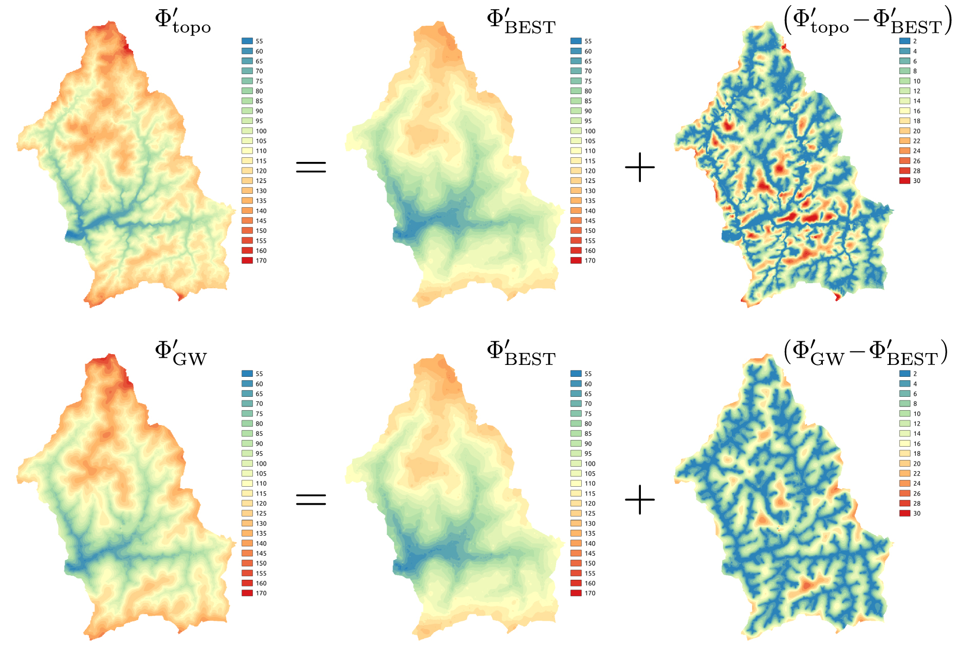
Decomposition of topographic elevation (
Decomposition of topographic elevation (
As can be seen on the figure, the topographic height above the envelope surface of talwegs (
From the point of view of catchment hydrological modeling, the kind of parsimonious and analytical reconstruction of the groundwater surface proposed in this study, as well as the identification of a conceptual, large-scale estimate of transmissivity
Codes used in this study are available in the author’s Basilisk sandbox at http://basilisk.fr/sandbox/nlemoine/AEM/envelope/envelope.c.
Conflicts of interest
The author has no conflict of interest to declare.
Acknowledgments
I would like to take the opportunity of this special issue to thank Ghislain de Marsily for all his incredible teaching, especially for passing on to students a taste for analytic approaches.
Vous devez vous connecter pour continuer.
S'authentifier