


 CC-BY 4.0
1. Introduction
In naturally fractured geological reservoirs, fluid-flow structure is a major question for hydrogeological modeling [Neuman 2005]. Especially for the crystalline rocks targeted for energy recovery exploitation, or geological storage of industrial wastes like CO2 or spent nuclear fuel, fluid flow only takes place in a tiny part of the whole rock, through the connected network of fractures between hydraulically active boundaries, while intact rock matrix permeability is considered as negligible. Fluid flow structure is hence a subpart of the fractured system.
While fractures are ubiquitous in crystalline rocks, the complexity of their spatial organization precludes the use of classical methods of homogenization to derive hydraulic properties for equivalent continuous media. Fracture systems result from long-standing geological histories and fracturing processes, leading to a complex multiscale structure. Fracture-size scales commonly cover several orders of magnitudes from fractures smaller than micrometers to millimeters to tectonic faults larger than hundreds of meters to kilometers with fracture size distributions adequately modeled by power-law distributions [Bonnet et al. 2001; Davy et al. 2013]. Their capacity to be hydraulically active is dependent on their topological structure (connectivity, intersections), their openness and transmissivity. These factors together contribute to present a very large variability—in space and intensity—of the inflows that can be measured at depth from flow logging [Follin 2008]. In parallel, usual data acquisition capacities are far from what would be needed to easily reduce modeling uncertainties for typical site conditions. These aspects contribute to the difficulty to define relevant models of the fluid-flow structure for naturally fractured rocks and emphasizes the need to model the discrete nature of the flow before deriving any homogenized properties.
Discrete Fracture Network (DFN) approaches emerged in the late eighties [Cacas et al. 1990a, b; Long and Witherspoon 1985; Long and Billaux 1987]. Since then, they are widely used and developed, most often for applications that involve hydrogeological and hydro-mechanical modeling, e.g. [Davy et al. 2006, 2018; de Dreuzy et al. 2013; Lei et al. 2017; Park et al. 2002; Selroos et al. 2022]. As they realistically reproduce the discrete nature of the flows—typically spacing between inflows ranging from a few meters to tens of meters along wellbore—they are the most suitable for understanding flow structures in-situ. They also permit aggregation of various types of data (geological, mechanical, hydraulic, etc.) in a multidisciplinary approach where the DFN is the unifying element, as part of a strategy to minimize modeling uncertainties [Selroos et al. 2022].
The major theoretical questions for hydrogeological modeling of fractured media, which directly drive and impact the flow structure modeling, are scale dependence and upscaling or homogenization. The issue of the scale dependence of the hydraulic properties is widely debated. One of the first compilations on that subject is the seminal paper of Clauser [1992] which compiled permeability measurements from lab to regional scales, emphasizing a permeability increase with scale increase up to a hundred meters. This conclusion has been questioned by Hunt [2003b], who posited that although experiments often indicate an increase in the hydraulic conductivity with increasing scale, this effect may be explained by sampling issues rather than intrinsic scale effect. Other studies, based on field observation [Illman 2006; Neuman 2003; Neuman and Di Federico 2003; Ren et al. 2021] or modeling [de Dreuzy et al. 2001b, 2002] are in line with the observations from [Clauser 1992] and a scale effect emerging from the fracture network connectivity structure and transmissivity distribution. Illman [2006] also observed a directional permeability scale effect in cross-hole test results and hypothesizes that the effect is controlled by the connectivity of fluid conducting fractures. A scale increase of effective permeability with scale is also shown in Martinez-Landa and Carrera [2005] and Ren et al. [2021] from single hole and cross-hole pumping tests data and identify a scale dependence likely site-dependent too. de Dreuzy et al. [2001b, 2002] use a DFN model (in 2D) for which the fracture length and fracture aperture distributions are power laws and study the resulting hydraulic properties as the flow structure and equivalent permeability. They determine the equivalent permeability scale effects, characterize the flow structure by a channeling indicator, and establish the relationship with the fracture distributions parameters. Upscaling permeability is an active research area in hydrogeology both for fractured and unfractured media. Upscaling consists of deriving the equivalent permeability from the smaller scale permeability distribution [de Dreuzy et al. 2010]. Wen and Gómez-Hernández [1996] and Renard and Marsily [1997] reviewed the state of the art on upscaling conductivities in heterogeneous media. Oda [1985] developed an analytical approach to define equivalent permeability from a DFN description based on geometric characteristics of fractures with arbitrary orientations. de Dreuzy et al. [2001b, 2002] develop the relationship between equivalent permeability and the parameters of multiscale DFN models in 2D and hence the scale dependency. Chen et al. [2015, 2018] develop numerical approaches to compute the equivalent permeability from a DFN description.
The question investigated in this paper is how to best use available hydro data for capturing the multiscale nature of in-situ flow structures and to derive manageable and relevant metrics for site modeling purposes. At the Forsmark area in Sweden, site investigations have been performed by Svensk Kärnbränslehantering AB (SKB), the Swedish Nuclear Fuel and Waste Management Company, for more than two decades in view of the future deep repository for spent nuclear fuel [Follin 2008; Follin et al. 2007; Selroos et al. 2022]. Follin et al. [2014] use flow logs and metrics based on the relative proportion of sealed, open, and flowing fracture frequencies together with equivalent transmissivity distributions to calibrate the parameters of DFN models for flow simulations. Maillot et al. [2016] compare the performance of different DFN models from the comparison of channeling and equivalent permeability indicators. Zou and Cvetkovic [2020, 2021] also use DFN models and varying hydraulic boundary conditions to simulate steady-state pumping tests and derive indicators of cumulative and of complementary cumulative distributions to evaluate the impact of fracture in-plane heterogeneities on the flow structure at the DFN scale.
The first objective of this study is to develop flow-based metrics adapted to in-situ flow testing capacities and suited to emphasize the multiscale nature of the flow structure. To address these issues, the database of fractures and discrete inflows at Forsmark, which includes flow logging and steady-state pumping tests, was analyzed with metrics revisited from the former work of Maillot et al. [2016]. The second objective is to test the capacity of the latter to discriminate between DFN models otherwise calibrated to similar geological and geometrical observations. A modeling environment is set up in the software “DFN.lab” to generate DFN realizations from a predefined range of DFN models and perform numerical flow simulations in steady-state pumping configuration simulations.
The paper is organized as follows: the data and conditions of the Forsmark site are recalled in Section 2. The framework to define the metrics is presented in Section 3. Data analyses are presented in Section 4. In Section 5 the DFN models are defined and finally, several a priori equiprobable DFN models are compared with each other and with the field data and the interpretations and comparisons between data and models are presented. Results and outcomes of the study are finally discussed in Section 6 and summarized in the conclusion. To facilitate ease of reading this study, specific parts have been moved to appendices.
Note that, while the analytical tools and methodology are generic, the results are specific to the studied area (mostly the Nordic granites). It is not presumed that thresholds and trends are generalizable to all crystalline rocks [e.g., Dewandel et al. 2006].
2. Site and available data overview
The Forsmark site in Sweden, located in crystalline bedrock in south-eastern Sweden and located roughly 130 km north of Stockholm, is selected by the Swedish regulatory authorities to build a nuclear waste repository for spent nuclear fuel at 470 m depth [SKB 2011]. Svensk Kärnbränslehantering AB (SKB) is in charge of site investigations, future construction, and long-term safety assessment of the final repository. The database built over the course of the site investigations encompasses data from geological, mechanical, hydrogeological, geochemical, etc., aspects. Several tens of boreholes each reaching lengths up to about 1 km have been drilled and exhaustively logged.
The presented analyses relies on a detailed description of the fracture transmissivity structure in the different boreholes that have been extensively carried out at the Forsmark site by SKB with the Posiva Flow Logs (PFL). PFL was originally developed by Posiva Oy to meet the demand on flow measuring techniques adapted to sparsely fractured rocks and low-permeability environments [Öhberg and Rouhiainen 2000]. The method couples a very low threshold for flow detection (down to 0.1 l/min) and a precise positioning of the device that allows them to detect single fractures inflow with a depth resolution of a couple of centimeters. The hydraulic properties of every cored borehole at the Forsmark site are hence tested [Rouhiainen and Pöllänen 2003; Rouhiainen et al. 2004] by performing a standard hydraulic test where the applied pressure head and resulting flow are recorded. The derivation of a transmissivity is based on the Thiem (or Dupuits) solution for steady-state radial flow without skin effect, so that the flow rate Q1 at a borehole test section of size L is equal to:
| (1) |
Q1: measured flow rate in the test section (m3∕s)
K: hydraulic conductivity of the test section (m/s)
L: length of the test section limited by packers (m)
R: radius of influence (500 m) (m)
r0: radius of the borehole (m)
h0: undisturbed hydraulic head far from test section (m)
h1: pump-induced or natural borehole hydraulic head (m).
The two unknowns K and h0 can be deduced from two pairs of hydraulic heads (h1and h2) and resulting flow rates (Q1 and Q2) provided that K is not dependent on the induced pressure (no hydromechanical effects).
A combination of sequential and overlapping flow logging allows identifying water conductive fractures down to a spatial resolution of 0.1 m and flow rates down to 30 ml⋅h−1. This leads to a measurement limit of approximately T = 10−10 m2∕s when expressed in equivalent transmissivity as defined below.
The transmissivity of a test section, or the fracture identified by the sequential mode, is defined as:
| (2) |
In practice, the same set of flow rate measurements is done twice all along a tested borehole: the first pass is for natural flow rate conditions (no pumping), and the second one is for a typically imposed drawdown of 𝛥h = 10 m.
The distribution of PFL transmissivities for all wells is given in Figure 1b. The log average is about 3 × 10⁻⁸ m2⋅s−1 with values ranging from 2.5 × 10⁻¹⁰ to 1.3 × 10⁻³ m2⋅s−1. The average intensity of PFL log-transmissivities does not vary significantly with depth (Figure 1c) in contrast to the density of PFL fractures, i.e., the number of fractures where a transmissivity has been detected, and to the transmissivity variability (Figure 1a). From these observations, we identify three main domains: the near surface (0–200 m), the domain of interest for the repository (200–500 m), and a deeper domain (>500 m). The near surface is highly fractured and highly permeable; the density of PFL fractures is 1 PFL every 5 m on average (Figure 1a). It is characterized by horizontal sheet joints, which makes them distinct from the deeper parts. The intermediate domain is rather homogeneous with a density of PFL fractures about half the near surface. The deep domain is very dry with only a few PFL fractures, on average 1 every 2T50 m.
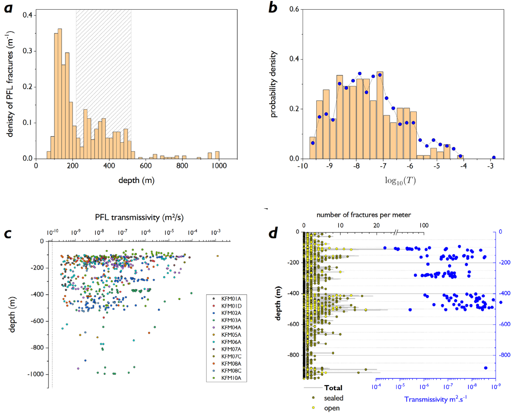
(a) (top left) Number of PFL fractures (i.e., fractures whose transmissivity is detectable with the PFL flow log) per 20 m depth increment. (b) (top left), Distribution of the decimal logarithm of PFL transmissivities in m2⋅s−1; the bars are for the whole domain (100–1000 m) and the solid blue dots for the target domain between 220 and 520 m. No value smaller than 10−9.5 are observed; the impact of this threshold, although very low, is discussed in Section 4.3 and in Figure 6. (c) (bottom left), PFL transmissivity as a function of depth for all the boreholes. (d) (bottom right), Example of a borehole logging (KFM02A) showing the measured density of fully intersecting fractures (number per borehole length with sealed and open densities indicated by the solid and yellow dot, respectively) on the left and the measured PFL transmissivity on the right. Masquer
(a) (top left) Number of PFL fractures (i.e., fractures whose transmissivity is detectable with the PFL flow log) per 20 m depth increment. (b) (top left), Distribution of the decimal logarithm of PFL transmissivities in m2⋅s−1; the bars are for the whole domain ... Lire la suite
The spatial distribution of transmissive fractures varies from one borehole to another but with common features as clustering in flow zones, presence of large domains without detectable flowing structures, and positive correlation between zones of high fracture density and zones of large PFL transmissivities (Figure 1d). Note that the correlation between fracture density and PFL transmissivity is far from perfect and many counterexamples exist where PFL fractures are observed corresponding to zones of normal fracture density.
In the following, we focus on the domain of interest for the waste repository. We arbitrarily set the upper and lower depths to 220 m and 520 m, respectively, in accordance with the density of the PFL fractures observed in Figure 1a. The distribution of PFL transmissivity between 220 and 520 m is not different from that observed on the whole domain (100–1000 m), despite the variability in the density of PFL fractures (Figure 1b).
3. Scaling metrics for flow log interpretation
In what follows, an interpretation framework based on the PFL data, including the transmissivity values and their spatial distribution is introduced. This is done through the prism of scale analysis, where the in-situ scale-dependent permeability is defined and evaluated for domains of increasing size.
The primary component of the analysis is the total inflow through a given core log section:
| (3) |
To reveal the flow network organization, we focus on the distribution of “wet” sections (i.e., sections containing at least one inflow), as it is done when determining the fractal properties of a network [Tél et al. 1989]. Whether a section is dry or wet depends on the resolution of the inflow measurement. Even if the PFL instrument is extremely sensitive, it is clear that the transmissivity distribution is not complete and truncated at the PFL resolution (Figure 1b). This issue will be discussed further down in the text.
By taking the geometric average of the section permeability, as in de Dreuzy et al. [2002], we expect to identify some important characteristics of the flow structure (Figure 2): the percolation threshold scale pc (transition between regime I and II in Figure 2), the permeability increase above pc (regime II), and possibly a Representative Elementary Volume (REV) that indicates the scale above which the permeability no longer varies. The correspondence between the percolation threshold and a scale was established for fracture networks with a power-law size distribution [Berkowitz et al. 2000; Bour and Davy 1997, 1998; Darcel et al. 2003b; de Dreuzy et al. 2000]. Compared to networks of constant size, the percolation threshold reflects the connectivity of small fractures and the probability of encountering fractures larger than the size of the systems that connect the networks on their own. It is this dual connectivity that makes connectivity scale-dependent and gives a correspondence between the percolation threshold and a given scale. Below the percolation threshold, the wet sections are likely containing one main fracture/channel with a permeability that decreases as
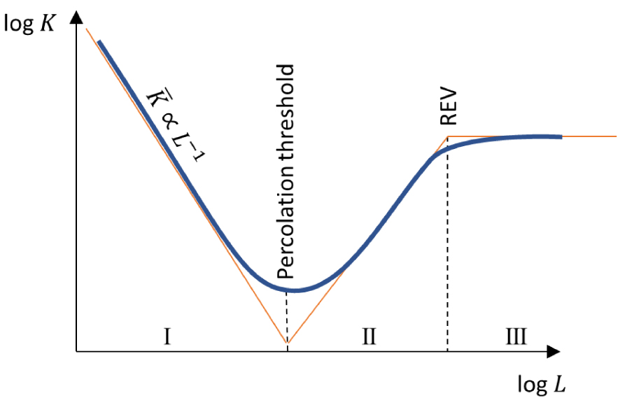
Schematic evolution of the geometric average of the permeability K as a function of the measurement scale L (solid blue line). The thin red segments indicate the three main regimes: below the percolation threshold scale pc (I), between pc and the representative elementary volume (REV) (II), and above the REV (III) [Charlaix et al. 1987; de Dreuzy et al. 2001b, 2002]. See text for an explanation of the three regimes.
To calculate K(L), we subsample each borehole with section lengths smaller than the total borehole length obtaining a set of equivalent hydraulic conductivities Kj (Equation (3)). We note N>0(L) the number of core sub-sections containing at least one positive inflow and hence a positive Kj.The first proposed metric, the function Ka(L), is the arithmetic average of the above-defined equivalent permeabilities derived from the ensemble of flowing core sections (non-flowing core sections are discarded) for a size scale L, as summarized in the equation below:
| (4) |
| (5) |
| (6) |
This metrics has been proposed by de Dreuzy et al. [2002] as the most representative mean for a permeability distribution that tends to be log-normally distributed (Figure 1).
Both Ka(L) and Kg(L) are likely to be dependent on the inflow detection limit estimated at 10−10 m2⋅s−1 for PFL measurements. Even if this value is very low, the transmissivity distribution in Figure 1b suggests that smaller values exist. By artificially increasing the detection limit, we test in the following section that the metrics do not depend too much on its value as long as it remains much in the lower end of the transmissivity distribution.
To characterize the flow channeling, we also calculate the average number of inflows in all flowing sections of length L, n(L), and a channeling metric nQ(L) derived from [Maillot et al. 2016]:
| (7) |
4. Hydraulic data interpretations
In this section, we compute the different metrics and indicators defined in the previous section for the datasets listed in Table 1 in the depth range 220–520 m (see Section 2 for an explanation of this depth range).
List of boreholes (IDCODES in the SICADA database) with PFL data including the total number of inflows, the depth of the uppermost and lowermost inflow, the smallest and the largest PFL transmissivity
| IDCODE | Number of inflows (T > 0) | Uppermost inflow (m) | Lowest inflow (m) | Min(T) (m2∕s) | Max(T) (m2∕s) | Total logged length (m) |
|---|---|---|---|---|---|---|
| KFM01A | 34 | 105.3 | 363.4 | 2.45 × 10⁻¹⁰ | 5.31 × 10⁻⁸ | 891 |
| KFM01D | 34 | 106 | 571.17 | 6.59 × 10⁻¹⁰ | 2.30 × 10⁻⁶ | 708 |
| KFM02A | 125 | 101.8 | 894 | 6.16 × 10⁻¹⁰ | 4.21 × 10⁻⁵ | 899 |
| KFM03A | 71 | 106.4 | 994 | 8.90 × 10⁻¹⁰ | 9.21 × 10⁻⁵ | 896 |
| KFM04A | 142 | 109.6 | 954.8 | 7.16 × 10⁻¹⁰ | 3.54 × 10⁻⁵ | 876 |
| KFM05A | 27 | 108.9 | 720 | 4.45 × 10⁻¹⁰ | 1.23 × 10⁻³ | 897 |
| KFM06A | 99 | 102.4 | 770.8 | 2.40 × 10⁻¹⁰ | 1.92 × 10⁻⁵ | 895 |
| KFM07A | 23 | 110.8 | 261.4 | 3.57 × 10⁻⁹ | 7.67 × 10⁻⁵ | 892 |
| KFM07C | 15 | 98.4 | 279.8 | 8.99 × 10⁻¹⁰ | 4.81 × 10⁻⁵ | 413 |
| KFM08A | 41 | 107.6 | 687 | 2.48 × 10⁻¹⁰ | 2.20 × 10⁻⁶ | 846 |
| KFM08C | 21 | 102.4 | 683.6 | 7.51 × 10⁻¹⁰ | 2.95 × 10⁻⁶ | 848 |
| KFM10A | 56 | 60.3 | 484.4 | 1.64 × 10⁻⁹ | 2.79 × 10⁻⁵ | 437 |
4.1. Permeability averages
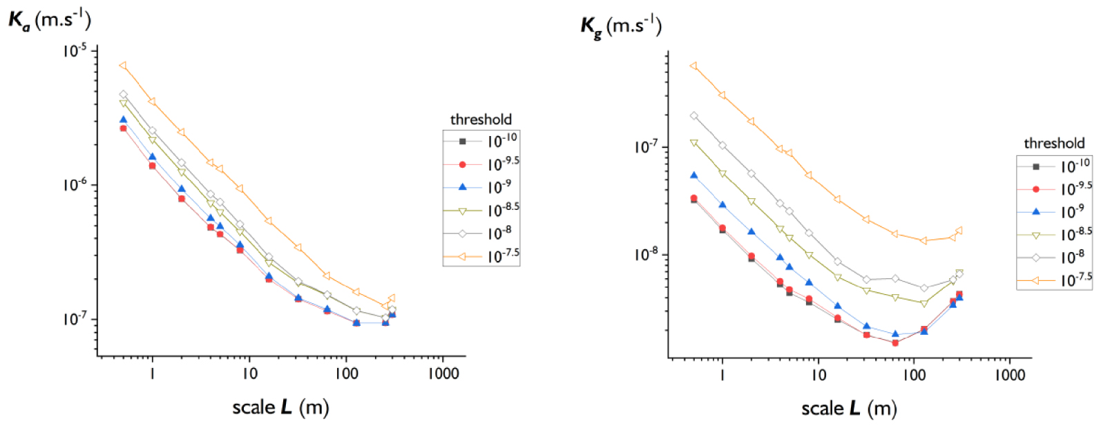
The scale evolution of equivalent arithmetic and geometric permeabilities are plotted in Figure 3. From borehole to borehole and comparable size scale, the calculated values are spread over 4 orders of magnitude. Despite this large dispersion, all the plots display a similar shape with a L−1 decrease over about 1 to 2 orders of magnitude when increasing scales until a stable (for Ka) or increasing (for Kg) regime is reached with large-scale permeabilities that range between 2 × 10⁻¹⁰ and 4 × 10⁻⁷ m⋅s−1. The transition between both regimes is at about 30 m for both permeability averages.
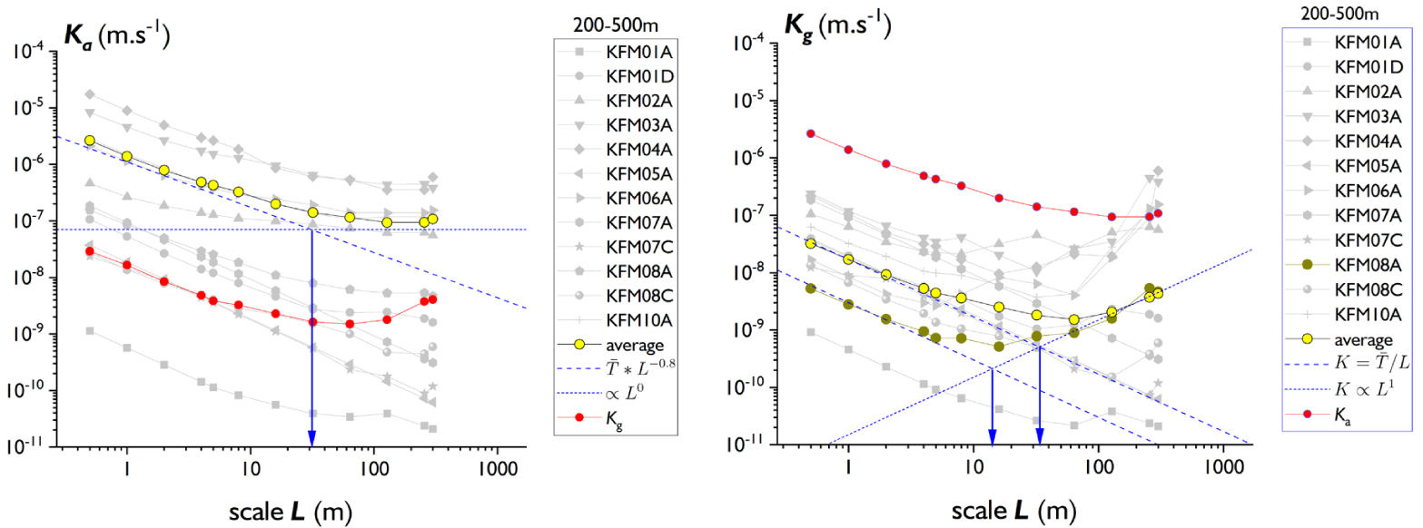
Ka(L) (left) and Kg(L) (right) computed for each borehole dataset listed in Table 1 (grey symbols) as a function of scale. For both, the yellow dots indicate the average of all boreholes and the red dots, the permeability average (i.e., Ka for the Kg graph and vice versa). The blue lines represent power-law fits at small and large scales, respectively. The dark yellow dots in the Kg plot are for KFM08A, a borehole that will be discussed in the modeling section. Masquer
Ka(L) (left) and Kg(L) (right) computed for each borehole dataset listed in Table 1 (grey symbols) as a function of scale. For both, the yellow dots indicate the average of all boreholes and the ... Lire la suite
The evolution of Ka(L) and Kg(L) reflects the organization of flows along the boreholes. In the first regime, as long as the length of the core sections is smaller than the minimum distance between two inflows, every element contains only one inflow and hence the equivalent permeability is inversely proportional to the core section length:
| (8) |
As expected, the arithmetic average of Kj is larger than the geometric average but the scaling trends are similar for this small-scale regime. We note that, for Ka, the average of all boreholes (yellow dots) seems to decrease slightly less than L−1, ∝L−0.8. This reflects a difference between the least and most permeable boreholes; the latter (KFM02A, KFM03A, KFM04A, KFM10A) having a less steep decrease with scale than the former. A basic explanation is that a high permeability is also associated with a higher density of inflows. This is not observed for the borehole-averaged Kg because the geometric average gives a more distributed weight to all boreholes whatever their permeability.
When the section length is large enough to gather several inflows, the permeability stabilizes with scale for the arithmetic average Ka, or grows as ∼L0.7 for the geometric average Kg as the result of the transmissivity distribution. The transition between both regimes spans over one order of scale magnitude between ∼6 and ∼60 m with a critical value at 30 m determined from the intersection of both end-member regimes (Figure 3). There is no limit to the increase of Kg with scale in this regime for the observed scale range (30–300 m), which means that a REV such as anticipated in Figure 2 is beyond 300 m, if it exists.
The average number of inflows per section confirms the trends observed on the permeability averages (Figure 4, left). For sections smaller than 4–5 m, only one inflow is observed on average per wet section, and then the number increases as L0.75. The maximum number of inflows for the largest section of 300 m varies between 10 and 80 with an average of 20, except for the two boreholes KFM01A and KFM07C where only 1 and 2 inflows are recorded, respectively. We also calculate the channeling metrics nQ (Equation (7)), which quantifies the number of main channels in each section. nQ shows the same two-regime scaling trend as the number of inflows per section but with smaller values, as expected. It increases above 4–5 m approximately as the square root of the number of inflows. For the largest section (300 m), only 3 main channels on average are detected.
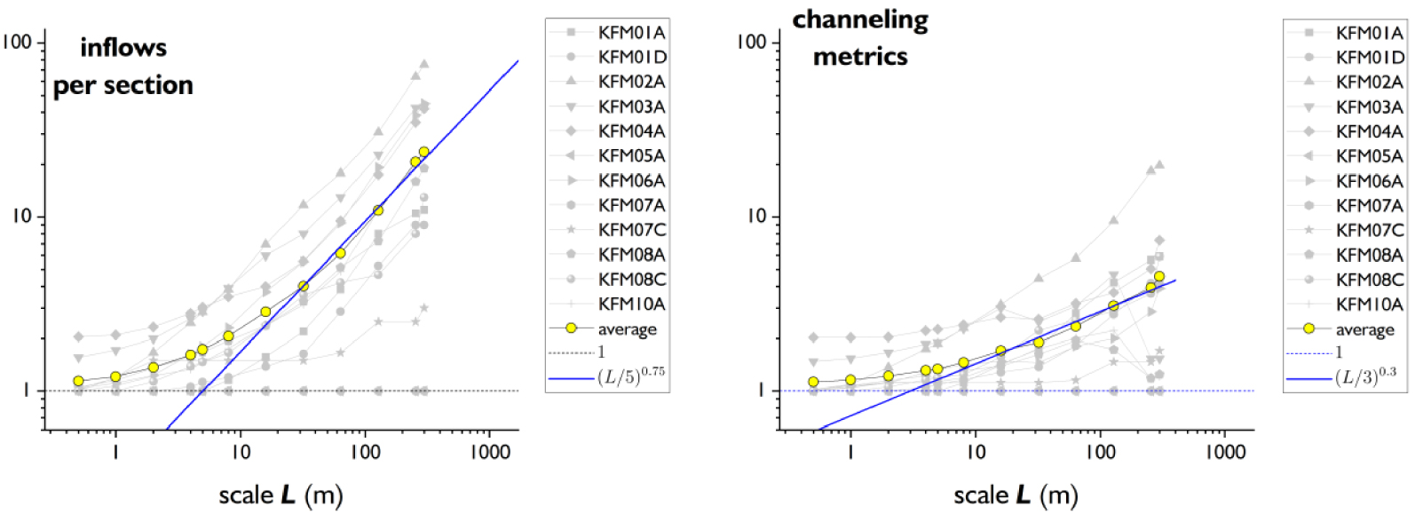
Plot of the average number of inflows per section (left) and of the channeling metrics defined in (7) (right) as a function of section scale.
4.2. Flow structure organization
We plot in Figure 5 the evolution with L of the ratio of the proportion of “wet” sections—i.e., number of sections that have at least one inflow divided by the total number of sections—with scale. This ratio, hereafter called the wetting ratio rw, controls the evolution of Ka(L) (see discussion above and (5)) and it can be used to identify a potential fractal nature of the flowing structure as it is classically done in box-counting methods [Mandelbrot 1982; Pavón-Domínguez and Moreno-Pulido 2022]. In a fractal of dimension D1D in 1D, the number of wet sections decreases as (L∕H)D 1D with H the investigated borehole length (here 300 m), and the wetting ratio increases as rw ∼ (L∕H)1−D 1D. D1D = 0 is a point-like structure in 1D corresponding to a plane in 3D. Figure 5 shows the two regimes already described: for scales smaller than ∼30 m, the wetting ratio increases as L corresponding to individual flow planes. Above 30 m, rw = (L∕H)0.3 indicating a fractal structure with a 1D dimension of 0.7 (2.7 in 3D). This complex structure and the distribution of transmissivity are likely to be responsible for the increase in the geometric average of permeability.
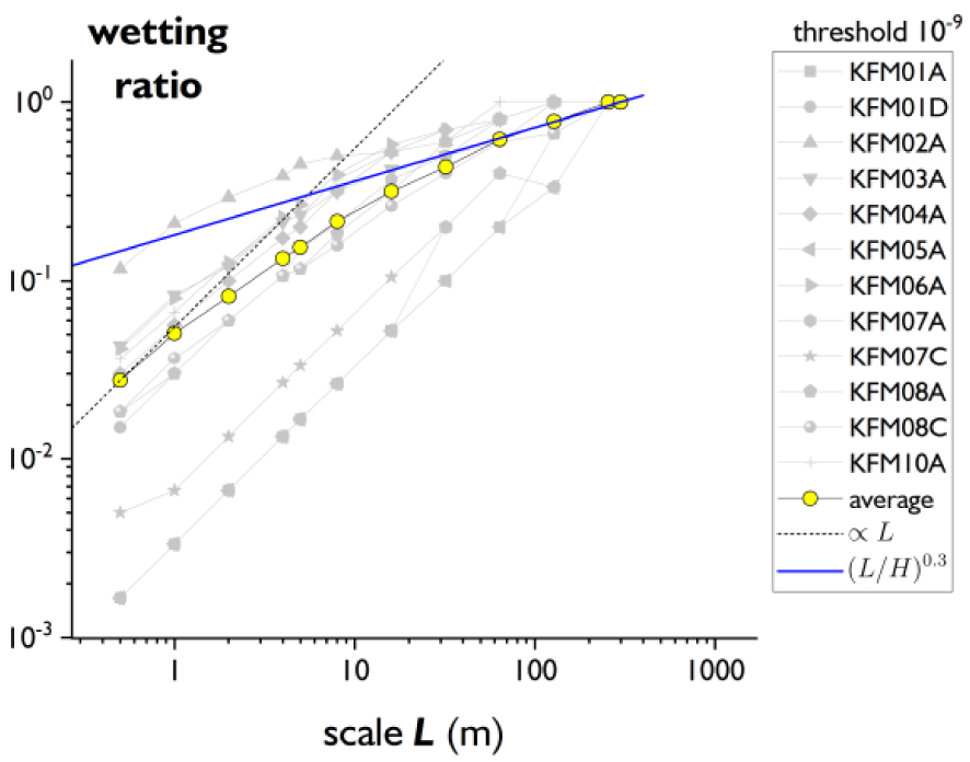
Evolution of the wetting ratio, i.e., the proportion of “wet” sections, i.e., containing at least one inflow, with section length scale L for all the boreholes (grey symbols) and for the average over all the boreholes (yellow dots). The scaling is L (dashed line) and L0.3 (solid blue line).
4.3. Dependency on the detection threshold of transmissivity
The previous analysis is potentially dependent on the flow detection resolution to identify wet and dry (no-flow detected) sections. Both Ka and Kg rely on the permeability of “wet” sections defined as the dual of no-flow sections. If inflows smaller than the detection limit of transmissivity exist, the number of wet sections will increase and the average permeability decreases. Even if the detection limit is very small, it does not seem to represent the lower bound of the transmissivity distribution (Figure 1b).
Considering that we cannot decrease the measurement resolution, we first apprise the reader that the previous scaling analysis is performed with a transmissivity threshold of 10−10 m2⋅s−1 and that the results may depend on this threshold. Then, we performed the same analysis as above but with different detection thresholds of transmissivity (Figure 6). The curves are identical for detection threshold (Td) up to 10−10 m2⋅s−1 and similar, i.e., presenting the same log-shape but with a higher permeability for Td up to 10−8 m2⋅s−1, which is the mode of the probability distribution of log-transmissivity. We thus conclude that the detection threshold is likely to be small enough to allow for a relevant scaling analysis of the flow structure, but we will be certain of this conclusion only if analyses were carried out with an even lower detection limit.
Evolution of the permeability averages Ka (left) and Kg (right) as a function of section scales for different transmissivity thresholds (see text).
4.4. Flow structure indicators
From the previous analysis, we identify a series of flow structure indicators which could serve as a basis for testing, and calibration of validating hydrogeological models. The indicators are best chosen to be characteristics of the fractured media that are likely to be controlling the flow properties, that can be measured, and whose measure is not too much affected by the conditions of the experiment. The 4 indicators listed below and in Figure 7 are chosen to be the measures of transmissivity distribution and flow structure.
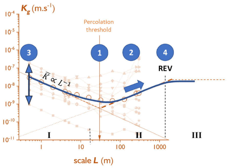
Representation of the 4 indicators (number in circles) described in the text with a graph which superposes the data of Figure 3 and the schematic scaling evolution of Figure 2. The first is the percolation threshold scale, the second is the permeability increase above the percolation threshold, the third is the distribution of transmissivities, and the fourth is the REV scale.
For each borehole, the equivalent geometric permeability average (6) with scale L can be characterized by a V shape (Figure 7) with a scattering from one borehole to another. These trends are basic to the definition of our 4 indicators.
The first indicator is the scale at which network percolates, which is about 30 m in the studied area. This scale also represents the average distance between inflows or inflow clusters. The evolution of Kg(L) below the percolation is representative of sections in which the number of inflows does not increase with scale, which explains the L−1 scaling.
The second indicator is the increase of the geometric permeability average with scale above the percolation threshold. It reflects the spatial distribution of inflows and the probability to encounter a flow path of large intensity when increasing the section scale. The slope of this increase is characteristic of the flow organization, a steeper slope indicating a higher heterogeneity of flows. Note that the increase of permeability with scale is long debated in the hydrogeological literature [Hunt 2003a, b; Illman 2006; Neuman 2005, 1994, 2003; Neuman and Di Federico 2003].
The third indicator is the dispersion of the borehole curves around the L−1 decrease. From borehole to borehole and comparable size scale, the calculated values are spread over 3 orders of magnitude (Figure 7). At sizes L smaller than the minimum distance between two inflows dmin, Kg(L) is simply equal to the geometric average of the set of individual transmissivities divided by L:
| (9) |
In theory, it exists a fourth indicator which is the representative elementary volume (REV), above which the permeability becomes scale independent. Figure 3 shows that the REV scale, if it exists, is larger than the investigated section length of 300 m.
5. Calibration/validation of DFN models
This section aims at testing the relevance of the indicators to calibrate, validate or reject DFN models. It should be taken as an illustration of the potential of the indicators and not as an in-depth analysis of the modeling.
The DFN modeling process presented here is in line with the DFN methodology defined in Selroos et al. [2022], where the definition of a DFN model for a hydrogeological application involves several steps. In the first, geological and geometrical data are used to define the DFN model of all the fractures, whatever their internal properties may be (by convenience hereafter referred to as geo-DFN). The second one is an in-between between geometric and hydraulic modeling steps. It consists in defining the DFN model of all open and partly open fractures, as a subpart of the geo-DFN model (by convenience hereafter referred to as open-DFN). Before even assigning transmissivity properties to the fractures of the open-DFN model, and hence defining the hydro-DFN model, the structure of the open-DFN model is critical for the flow: having a connected path of open fractures between hydraulically active boundaries is the prerequisite to define hydraulic properties. In each step of the modeling process, data are integrated with prior models and hypotheses and evaluated in a cycle of Sensitivity Analyses, Calibration, and Rejection tests Selroos et al. [2022].
In this section, we present only a small part of this modeling process which focuses on the integration of hydrological data analyzed in Section 4. The other parts are only briefly described. The analysis focuses on the fracture domain FFM01 [Follin et al. 2014; Olofsson et al. 2007], which is the target geological formation for the spent nuclear fuel repository [SKB 2011]. Models are compared with the borehole KFM08A (Figure 3b, dark yellow dots) that is representative of FFM01.
5.1. Description of the selected models
The geo-DFNs rely on site investigations and data interpretations at the Forsmark site [Darcel et al. 2009; Fox et al. 2007; Olofsson et al. 2007]. The fracture density and fracture orientation distributions are measured from borehole logging and core mapping. The number of fractures fully intersecting the boreholes per unit core length P10 is converted into total surface of fracture per unit volume P32 by means of stereological rules [Dershowitz and Herda 1992; Darcel et al. 2003a; Davy et al. 2006; Piggott 1997]. The values of P32 for the different orientation poles recorded in Forsmark are given in Table 2 with references therein.
List of the different fracture sets for the FFM01 fracture domain at depths between −200 and −400 m with their intensity P32 and the Fisher parameters that define their orientation distributions
| Set name | P32 (m2∕m3) | Fisher distribution parameters | ||
|---|---|---|---|---|
| Trend (°) | Plunge (°) | Kappa (-) | ||
| NS | 1.292 | 292 | 1 | 17.8 |
| NE | 1.733 | 326 | 2 | 14.3 |
| NW | 0.948 | 60 | 6 | 12.9 |
| EW | 0.169 | 15 | 2 | 14.0 |
| HZ | 0.624 | 5 | 86 | 15.2 |
The multiscale organization of fracture networks is a critical attribute for fracture connectivity and flow [Bonnet et al. 2001; Bour and Davy 1998; Davy et al. 2006]. It results in fractal properties and power law fracture size distributions, which are confirmed by the analysis of outcrop and lineament trace maps [Darcel et al. 2009]. Davy et al. [2010] have shown that the outcrop data in Forsmark are consistent with a kinematic model of fracture nucleation, growth and arrest (hereafter called the UFM model). The resulting fracture-size distribution is a double power law with a scaling exponent close to −4 above a critical fracture size lc and −3 below. The geo-DFN relies on the genetic UFM model with rules given in Davy et al. [2013]; it is characterized by the critical fracture size lc, which fixes the fracture density P32; the larger is lc, the smaller is P32.
The open-DFN is a subset of the geo-DFN where only open fractures—i.e., fractures with a non-nil open aperture—are represented. The only data available is the surface ratio of open fractures (hereafter referred as the open fraction fop), which is varying between 0.15 and 0.25 in the geological formation [Follin et al. 2014; Olofsson et al. 2007] with a value around 0.15 for the target fracture domain FFM01 [Doolaeghe Wehowsky 2021]. fop can be measured from the core logging by identifying open and partially-open fractures and measuring the ratio of fractures presenting open voids, but this is a bulk ratio that does not indicate how the fractures are opened individually or depending on their characteristics. We suspect that the relationship between the open fraction and the fracture attributes (size or orientation) is a key parameter to define the hydraulic properties of the open-DFN.
We analyze different models for the distribution of the open fraction in the network, whose parameters are given in Table 3. In all the models, we assume that fractures are either completely open or sealed. The first two models—further referred as “lc-open”—are built as genetic UFM models [Davy et al. 2013] with a larger critical fracture size lc than the geo-DFN to account for the decrease of fracture density P32. The first and second models differ by the proportion of open fraction. The second model—further referred to as 𝛼-open, is a geo-DFN for which a number of fractures have been removed to account for the open fraction independently of their size (Figure 8b). The last model, originally presented in Follin et al. [2014], relies on a different approach where the geo-DFN step was skipped and a open/hydro DFN was directly generated with only a single power-law fracture size distribution and no genetic base but only Poisson-point processes (no spatial correlations between fractures), with the orientation of Table 2 [Follin et al. 2014]. For simplicity, this last model is named pp-open (pp for poisson-point). The size distribution and the open fraction of the Geo-DFN, lc-open, 𝛼-open and pp-open models are given in Figure 8 and the other model characteristics summarized in the legend of Table 3.
Parameters of the open-DFN models
| Model | Open fraction | pP32 borehole scale | Fracture size distribution |
|---|---|---|---|
| Geo-DFN | 0 | 4.6 | UFM size model, lc = 3.2 m |
| lc-open 25% | 0.25 | 1.2 | UFM size model, lc = 17.6 m |
| lc-open 21% | 0.21 | 1 | UFM size model, lc = 21.7 m |
| 𝛼-open | 0.25 | 1.2 | UFM size model, lc = 3.2 m |
| pp-open | 0.21 | 1.02 | Power-law, exponent −3.4 |
The open fraction and P32, which are scale-dependent parameters, are calculated for a fracture size of 0.076 m equivalent to the borehole diameter. Both parameters are thus comparable to field measurements. For all the models, the smallest fracture for flow calculation is 2 m, and the system is a cube of 150 m side. The number of fractures is between 37,000 and 70,000 depending on the open-DFN model.
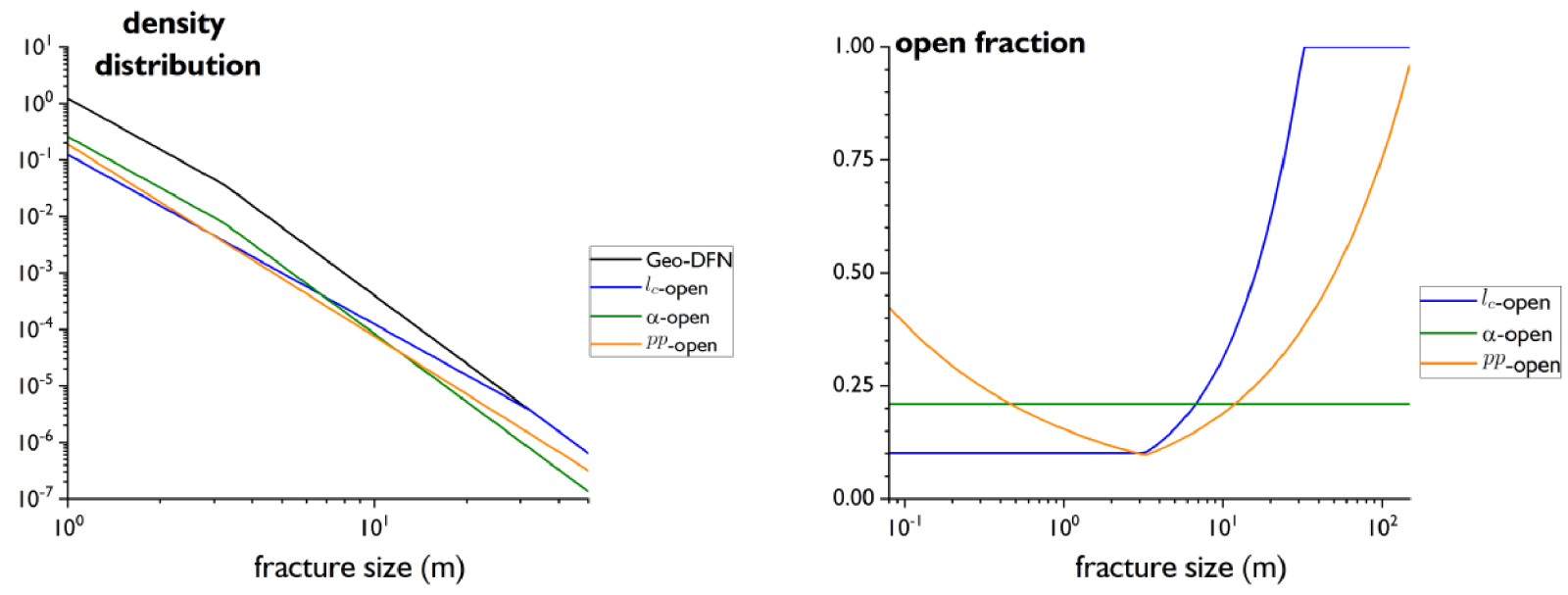
Density distribution (left) and open fraction (right) as a function of the fracture size for the Geo-DFN, lc-open, 𝛼-open and pp-open models, respectively.
Although the 4 DFN models are consistent with the same data, they are very different in terms of connectivity, as highlighted by the analysis of the percolation parameter p as a function of system size L (Figure 9). This parameter measures the degree of connectivity of the networks and is expressed as [Charlaix et al. 1984; de Dreuzy et al. 2000]:
| (10) |
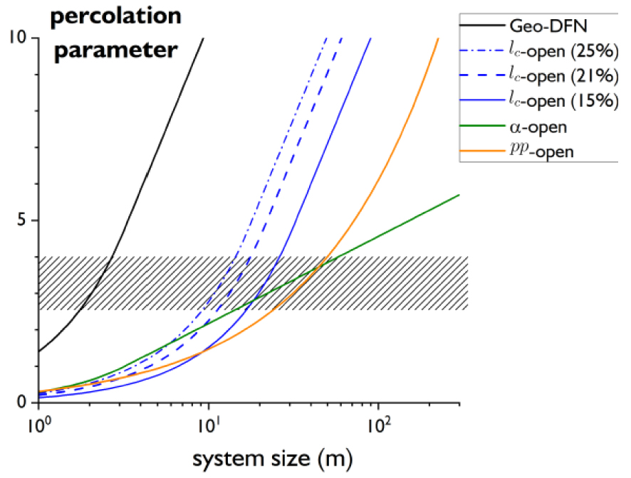
Evolution of the percolation parameters as a function of the system size for the Geo-DFN, lc-open, 𝛼-open and pp-open models. The expression of p is given by (10). The dashed rectangle indicates the percolation threshold for the prescribed orientations.
The Hydro-DFN is defined by assigning a transmissivity for each fracture. We define 4 different transmissivity models:
- all fractures have the same transmissivity (T = 1)—in this case, the resulting permeability is called the effective connectivity [de Dreuzy et al. 2001a]—;
- fracture transmissivity is proportional to the fracture size (T = l), which is the standard model studied by Frampton and Cvetkovic [2010] for similar geological formations;
- fracture transmissivity is a function of the normal stress applied to the fracture (T = f(𝜎n)); it mimics the closure of fractures by the normal stress to the fracture plane 𝜎n; in practice, 𝜎n is calculated from the projection of the remote stress tensor
with 𝜎c = 4 MPa; - fracture transmissivity is assumed to be the product of the two previous relationships, i.e., fracture size and stress: T = lf(𝜎n).
This list does not cover the whole range of model possibilities but it gives good examples of the types of transmissivity relationships that could be investigated for a site modeling. Note that, in these relations, the transmissivities are relative with respect to a reference value that must be calibrated to the data. The following analysis is independent of this reference.
5.2. Comparison models/data, and sensitivity analysis
Flow simulations are performed with the computational suite “DFN.lab” [Le Goc et al. 2019], according to the setup described in Appendices A and B. Results are averaged from 10 realizations for Kg (6) and the value is normalized by the permeability calculated first for a scale of 0.5 m:
Figure 10 shows the effects of the transmissivity model on the evolution of
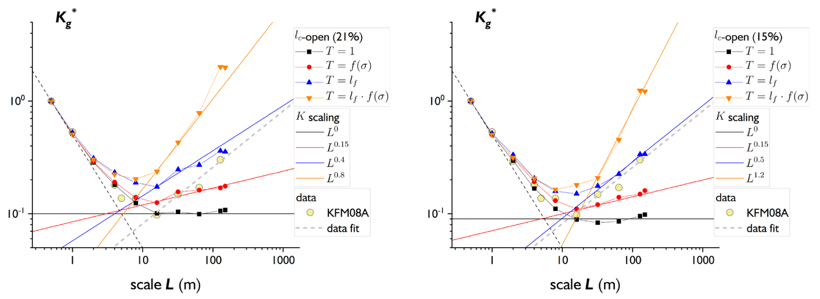
Evolution of the geometric averaged permeability as a function of scale for the lc-open model 21% (left) and 15% (right) with the various transmissivity models (see the list above). An approximate power law fit for the different regimes of scaling is provided for all the models. The fit exponent is an indication of the intensity of the permeability with scale for large scales. The permeability scaling measured at KFM08A (yellow dots) and the fit for large scaling (grey dashed lines) are also indicated for comparison. Masquer
Evolution of the geometric averaged permeability as a function of scale for the lc-open model 21% (left) and 15% (right) with the various transmissivity models (see the list above). An approximate power law fit for the different regimes ... Lire la suite
The transition scale between both regimes has been estimated from the intersection of the end-member regimes at small and larges scales: K ∝ L−1 at small scales, and K ∝ L𝛼 at large scales with 𝛼 dependent on the transmissivity model. The transition is about independent of the transmissivity model around 4–4.5 m for the lc-open model with an open fraction of 21% (Figure 10a) and around 10 m with 15% (Figure 10b). It is slightly larger than—but still consistent with—the percolation scale for this model estimated from Figure 9.
These simulations are merely indications of the possible effects associated with the transmissivity models. A more complete study is needed to derive general laws. Note also that the normalization by the first point of the curve removes the variability from one model to another and from one realization to another. This point is discussed later.
How the permeability scaling reveals the open-model is presented in Figure 11 for two transmissivity models: T = 1 (left) and T = lf(𝜎) (right). The trends are similar to those presented in Figure 10, and the differences between the different open models mostly lie in the scale at which the transition between both two end-member regimes occurs. The increasing order of the different transition scales is in agreement with the evolution of the percolation parameter with the scale: lc-open models first, then pp-open model and 𝛼-open. Even the crossing of the curves of the last two models observed on
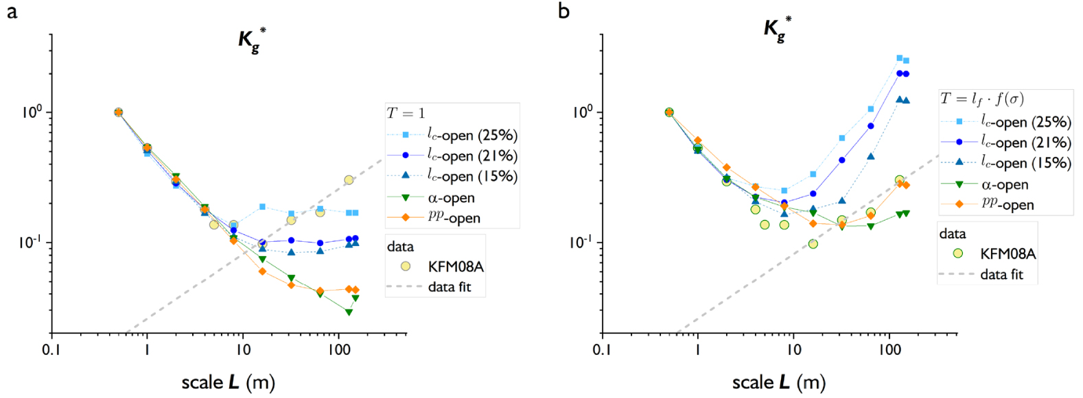
Evolution of the normalized geometric-averaged permeability for the different open-models and two transmissivity models: T = 1 (left) and T = l ⋅ f(𝜎) (right). The symbol colors and line types are similar to the one used in the Figure 9. The yellow dots on the right plot indicate the KFM08A scale analysis.
In Figure 12, we present an attempt to estimate the model variability (third validation indicator in Section 4.4). We calculate the lognormal standard deviation of the geometric average permeability 𝜎ln (K g) for 10 realizations for models, and in-between boreholes for data. 𝜎ln (K g) is dimensionless and does not depend on the unit of the fracture transmissivity, which makes it a useful indicator for comparing models and data. 𝜎ln (K g) has been calculated for 10 realizations for each combination between an open model and a transmissivity model. Figure 12 shows the evolution of 𝜎ln (K g) with scale for different transmissivity models and lc-open 15% (left), and for different open models and T = lf f(𝜎) (right). Not surprisingly, the transmissivity model with the largest variability is T = lf f(𝜎), i.e., when the transmissivity depends both on stress and fracture size. This is the only model that shows an increase in variability with scale above 10–20 m. This trend is also observed in the data but to a lesser degree. For all other transmissivity models, the variability is about constant with scale and it is not very different from one model to another except for the model with a constant transmissivity which has a lower variability (Figure 12a). This result must be confirmed by a larger number of simulations.
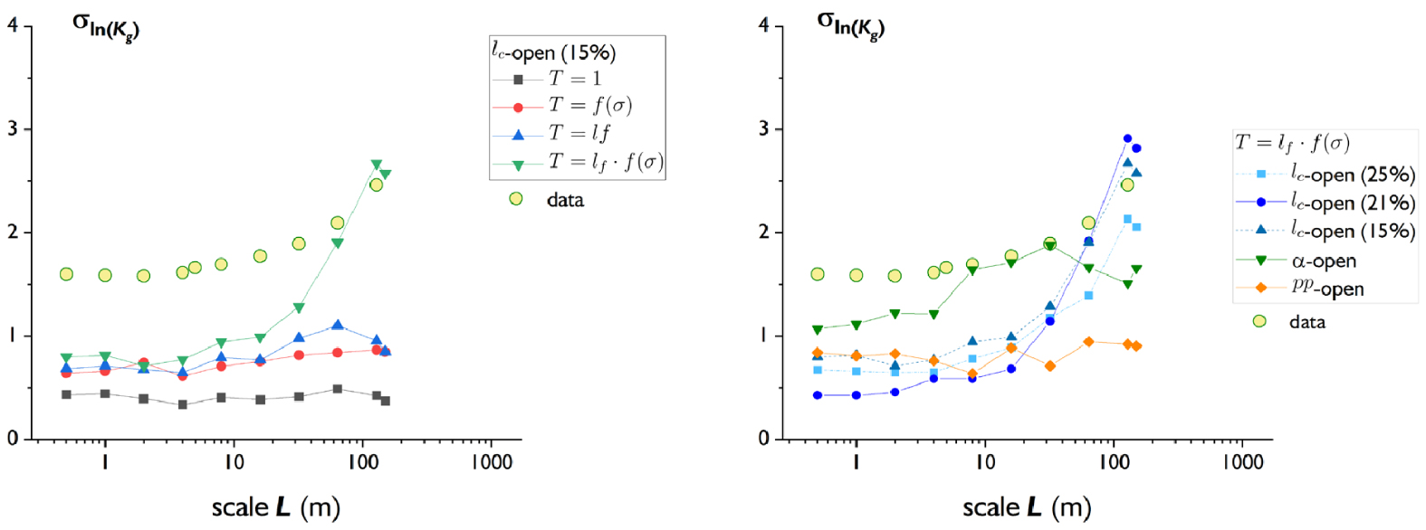
Evolution of the standard deviation for 10 realizations of the lognormal distribution of permeability as a function of scale. Left: comparison of the different open-DFN models, all with the transmissivity model T = l; right: comparison of the different transmissivity models, all with the lc-open DFN model.
The impact of the open model on 𝜎ln (K g) is presented in Figure 12b. The 𝛼-open model has the largest variability, probably because it is largely controlled by a few big fractures. The pp-open model is the only one where the variability does not increase with scale for this transmissivity model.
Note that the comparison between model and data is not fair because the boreholes mix domains that can be quite heterogeneous, in particular, in terms of open fraction, while models are built with a constant open fraction. The 𝜎ln (K g) values are therefore likely to be overestimated for the data compared to the models and a correction may be necessary to make a true comparison.
6. Discussion
The four indicators defined in the Section 4.4 turn out to be useful to validate or calibrate models. All the models presented are consistent with the data, but no all of them can reproduce the data indicators. We discuss here the ability of the indicators to constrain both the structure that carries the flow and the transmissivity model that is applied to that structure.
All the models—again, calibrated on the data from Forsmark—reproduce the V-shape scaling curve of the permeability geometric average observed in data.
- The first indicator is the scale which marks the transition between the L−1 scaling at small scale and the transmissivity scaling at large scale. This scale is closely related to a connectivity threshold of the open-DFN structure. Indeed, for open-DFN, whose distribution of the largest fractures follows a power law, the connectivity increases with scale and the percolation threshold is reached at a given scale which can be predicted by the evolution of the percolation parameter with the scale. For all the tested models, the transition/percolation scale seems to be independent of the transmissivity model.
- The second indicator is the increase of the geometrically-averaged permeability with scale. It can be modeled by a power-law scaling whose exponent gives the increase in intensity. This indicator reveals the transmissivity model and a large increase is likely associated with a dependency of fracture transmissivity with fracture size. A high variability in fracture transmissivity, even without this transmissivity scaling effect, can also create an increase in permeability but to a lesser extent.
- The third indicator is the variability of geometrically-averaged permeability from one well to another (data) or from one realization to another (models). It has been quantified as the standard deviation of the logarithm of permeability, which is a dimensionless parameter that relies on the likely lognormal permeability distribution. This indicator is much more sensitive to the structure model (open-DFN) than the transmissivity model with the exception of the extreme transmissivity model T = l ⋅ f(𝜎), where the variability is high and scale dependent above the transition scale (i.e., 2nd indicator) as it is the case for the data. We do not want to draw definitive conclusions on this indicator because it would require many more models and realizations, and a comparison taken on more homogeneous data.
Although the analysis is far from exploring all the structure and transmissivity models of DFN, we can draw few preliminary conclusions on the capacity of the chosen models to reproduce the indicators.
- In the DFN modeling workflow, an underconstrained critical point is the way in which the open fracture fraction is distributed in the network. Only the total open fraction cannot be retrieved from flow logs. If the open fraction is uniformly distributed over all fractures regardless of their size or orientation, as it is for the 𝛼-open model, the network is less connected than other models, and probably the natural networks, whatever the assigned transmissivity model may be (see Figure 8a). On the other hand, if the open fraction is large at small scale, as it is for the pp-open model, the network is more connected than other models and data at these scales. This highlights the primary importance of properly defining what fractures are sealed and the proportion of open fractures per fracture size.
- The transmissivity model T = 1 (i.e., constant transmissivity for each fracture) cannot not reproduce the V-shape of Kg vs scale. This model is obviously unrealistic, however we suspect that any transmissivity model, whose variability from one fracture to another is too low could not reproduce the permeability increase with scale as observed in data above ∼10 m. On the other hand, the transmissivity model combining fracture size and normal stress T = lf(𝜎) predicts permeability increase with scale too sharp compared to data. It is not certain to find an unequivocal solution between the transmissivity model and the observed permeability scaling by playing on the fracture size and orientation/stress dependence, but this indicator still reduces the field of possibilities.
- It is difficult to know at present whether a model should be rejected altogether (e.g., the 𝛼-open or pp-open models) or whether it is still possible to modify some of their parameters to fit the data. This exercise is however necessary to limit the field of possible models.
- The best-fit model among those tested is lc-open with a transmissivity model T = l but it is not totally satisfactory, particularly in terms of the variability it induces (3rd indicator), which is too low and does not depend on the scale.
Note that the fourth indicator, which is the existence of a representative elementary volume, is not observed in the data where the permeability geometric average increases continuously with the scale.
7. Conclusion
The objective of the paper is to better understand and quantify the flow structure in fractured rocks from PFL flow logs, and also to propose relevant indicators for validating, calibrating or even rejecting hydrological models. The data consists of a series of inflows along each borehole with an equivalent transmissivity measured from pumping tests. We first studied what the inflow distribution tells us about the permeability structure from a series of analysis: distribution of transmissivities as a function of depth, proportion of flowing sections as a function of section scale, scaling of the arithmetically-averaged and geometrically-averaged permeability. We argue that the permeability scaling evolution provides more information on the flow structures than macroscopic values (i.e., large scale permeability), the latter being too integrative.
We thus define three indicators of the flow structure from the scale evolution of the permeability geometric average that highlight intrinsic properties of the flow structure:
- a percolation scale ls,
- the way permeability increases with scale above ls,
- the permeability variability, measured as the standard deviation of the permeability logarithm for different boreholes or model realizations, as a function of scale.
A 4th indicator on the representative elemental volume could in principle be defined but the data show that this volume/scale is beyond the 300 m investigated.
We tested a series of numerical models by running flow simulations on generated DFNs to compute the same indicators on synthetic data. Most of the models are built from the DFN methodology with three steps: the geo-DFN based on the observed fracture network, the open-DFN which is the part of the geo-DFN where fractures are open, and a transmissivity model applying on each fracture of the open-DFN. The analysis of the models showed that the percolation scale is controlled by the open-DFN structure and that the percolation scale can be predicted from a scale analysis of the percolation parameter (basically, the third moment of the fracture size distribution that provides a measure of the network connectivity). For the same geo-DFN, the distribution of the open fraction with fracture size is the critical parameter that controls the percolation parameter and the percolation threshold. The way permeability increases with scale above the percolation threshold is controlled by the transmissivity model. We have tested several of them with a dependence of the fracture transmissivity on either the orientation of the fractures via a stress-controlled transmissivity or their size or both. Although size dependence induces the greatest effect on permeability increase, the variability due to orientation (i.e., stress) dependence also has a non-negligible effect that is enhanced when the two dependencies are combined.
The comparison with data on the first two indicators shows that a model that matches the characteristics of the geo-DFN with the measured open fraction of 15% adequately fits the data, provided that the large fractures remain open and that the fracture transmissivity model is well selected. Most of the other models shows unacceptable differences with data, however other models or model combinations still have to be explored before rejecting them.
The third indicator on model variability is still problematic since the natural data show a higher variability than the models but the open fraction is also much more variable in the data than in the models.
By characterizing the flow structure in terms of permeability scaling and variability, and by defining three indicators that describe some fundamental characteristics of the flow/permeability whatever the scale may be, we bring a new way to calibrate and/or validate models or at least to reduce the field of model possibilities.
Conflicts of interest
Authors have no conflict of interest to declare.
Acknowledgements
The authors acknowledge the two anonymous referees who helped improve the manuscript. Philippe Davy is particularly grateful to Professor Ghislain de Marsily for the help and encouragement to develop the fundamental research on the flow properties of fractured media.
Vous devez vous connecter pour continuer.
S'authentifier