


 CC-BY 4.0
1. Introduction
The low-carbon transition requires an increasing amount of raw materials, from the most traditional, such as aggregates, to the most emerging and rare metals, raising the question of their availability [de Marsily and Tardieu 2018]. In particular, sand and gravel will be needed for large-scale infrastructure development such as for wind turbine foundations and structures or for insulation materials. Although sand is one of the most abundant materials on Earth [Sverdrup et al. 2017], its exploitation faces major environmental issues, associated economical difficulties and even regional scarcity concerns [Ioannidou et al. 2020], in particular when it comes to its quality requirements. Population growth, rapid urbanisation and infrastructure development have led to increasing demand since the 1950s [OECD 2019]. Mostly used in the construction industry as a key ingredient in the production of concrete, for road bases and land reclamation, sand and gravel are the world’s most consumed primary materials after water, up to 50 billion tonnes produced each year [Bendixen et al. 2021], at unsustainable levels far greater than their natural renewal [Bendixen et al. 2019; Peduzzi 2014].
Sand and gravel resources are derived from various geomorphological settings such as beach deposits, streambeds, river floodplains and terraces, alluvial fans, and glacial deposits. Extraction of material from terraces and upland areas is generally perceived as having less impact than removing sand and gravel from active floodplains and stream channels [Kondolf 1997; Sandercock and Ladson 2014]. However, when aggregates are mined below the water table, artificial water bodies fed by groundwater appear as a new landscape feature. These thousands of gravel pit lakes are now a common freshwater lake type significantly influencing the morphology of the watershed, the natural hydrologic system and regional biogeochemical cycles [e.g., Mollema and Antonellini 2016]. In these environments, surface water and groundwater will mix and interact with the atmosphere. By offering open water surfaces where direct evaporation can occur, sustained by groundwater inflow, gravel pit lakes are generally recognised as a sink for adjacent aquifers in temperate and Mediterranean climates [Mollema and Antonellini 2016], particularly in dry years [Schanen 1998], although they may also act as a temporary buffer reservoir [Sinoquet 1987], especially during low-amplitude floods [Czernichowski-Lauriol 1998]. This freshwater loss is of concern, in areas where the mining of sand and gravel from those productive reservoirs is already in competing use with drinking water supply.
Furthermore, gravel pit lakes, characterised by infinite transmissivity and a unit storage coefficient, also alter the hydraulic gradient in the adjacent aquifer, causing the water table to rise or fall and thus disturbing the groundwater drainage pattern [Peaudecerf 1975]. By establishing a surface of equipotential head, gravel pit lake levels may nonetheless be representative of the average groundwater level, like giant piezometers. With the development of ever more efficient remote sensing systems, satellite observation will soon provide regular monitoring of temporal fluctuations of open continental water surfaces with unprecedented precision. Despite their small size, gravel pit lakes are a good candidate for future monitoring by the SWOT (Surface Water and Ocean Topography) satellite [Ottlé et al. 2020]. For landscapes where few in situ groundwater level measurements are available, gravel pit lakes could be used as proxy indicators of local water resource trends. This will require the use of a modelling tool for the coupled gravel pit-aquifer system.
A lot of effort has recently been put into analysing lake–aquifer interactions but future work still needs to assess the potential of using the lakes, and in particular the increasingly common gravel pit lakes, as monitoring wells of shallow groundwater for better water resources planning and management [Shrestha et al. 2021]. Understanding how gravel pit lake level will fluctuate in response to groundwater exchange, overland flow and atmospheric conditions (precipitation and evaporation) is therefore fundamental for this purpose, especially as artificial lakes interact differently with groundwater compared to natural lakes [El-Zehairy et al. 2018]. Special emphasis in this paper is on the dynamics of these interactions. By first reviewing the results of field and numerical studies, we recall which consequences gravel mining may have on groundwater systems from a quantitative point of view. We then present the numerical code we have developed in order to simulate the gravel pit lake/aquifer interaction and introduce the test case used to validate the lake module. On the basis of the same test case, we finally illustrate numerically the hydrodynamic effects associated with gravel pit lakes and also discuss the main factors influencing lake level changes.
2. A brief review of the hydrodynamical impacts of gravel pit lakes
The interactions between gravel pit lakes and their environment have received attention for many years and have recently been summarised by Mollema and Antonellini [2016]. This additional state of knowledge report is meant to be an overview of relevant information on the hydrodynamic aspects associated with the presence of gravel pit lakes. The main elements discussed in this section are summarised in Figure 1.
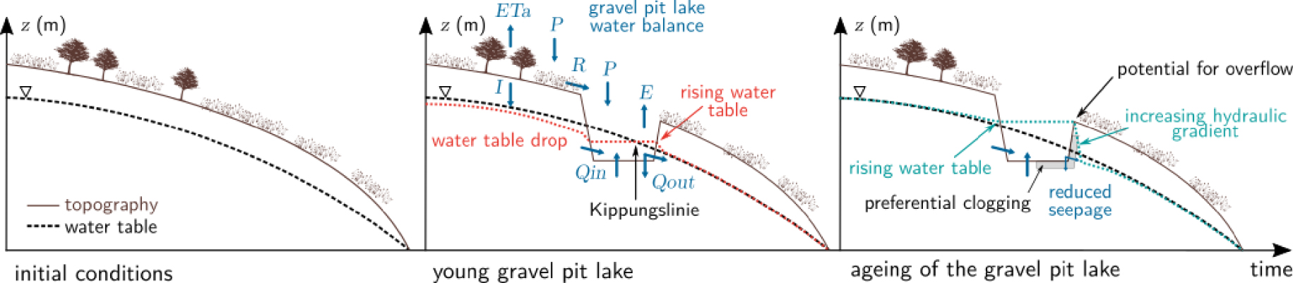
Illustration of gravel pit lake–aquifer interactions over time. The terms of the water balance are: precipitation P, land actual evapotranspiration ETa, open-water evaporation E, diffuse runoff R, infiltration I, groundwater inflow Qin, groundwater outflow Qout.
2.1. Characteristics of gravel pit lakes
By definition, a gravel pit lake develops where sand and gravel extraction extends below the water table. Gravel excavations are therefore typically found in areas with a shallow water table, in floodplains and adjoining terraces of large rivers, in glacial valleys or coastal areas, where most coarse-grained sediments were deposited. Scattered throughout these landscapes, pit lakes are permanent water bodies of recent formation, mostly dredged since the second half of the last century. Usually located near urban areas, where aggregates are needed, water-filled pits are used for a variety of purposes, as reservoirs for water supply and irrigation, for recreational activities, and wildlife habitat. As such, they play an important ecological role [Seelen et al. 2021].
The gravel pit pools are usually small, with a surface area varying from a few hundred square metres to several hectares. Many of them have steep sides, uneven but relatively flat bottoms and irregular shorelines [e.g., Hindák and Hindáková 2003; Kondolf 1997]. Their maximum depth depends on the thickness of the gravel layers, which is usually limited, resulting in generally shallow lakes but they tend to be deeper that natural lakes [Vucic et al. 2019] and some can reach a depth of several tens of metres [Mollema and Antonellini 2016].
Gravel pit lakes are often in close proximity to each other, with large areas of the plains turning into open pits, up to nearly 25% [Peckenham et al. 2009], but they are usually disconnected from permanent watercourses, except during exceptional floods [Kondolf 1997]. They therefore generally have no natural surface inlet and outlet. When they are located in relatively flat floodplains, diffuse runoff is also limited. In contrast, they are in close hydrologic continuity with the surrounding groundwater body [Søndergaard et al. 2018], as highly permeable sand and gravel deposits allow significant groundwater seepage. Groundwater inflow is thus considered a key component in the water balance of quarry lakes. This inflow returns either downstream to the aquifer or to the atmosphere, making most of these artificial lakes so called flow-through or seepage lakes [Wilson 1984].
2.2. Hydrodynamic effects associated with gravel pit lakes
Gravel pits are young objects in the landscape whose environmental effects have been observed in situ for about 50 years. A number of studies on their hydrodynamical impacts have been published since the pioneering work of Peaudecerf [1975] and Vandenbeusch [1975] in France, Wrobel [1980] in Germany or Wilson [1984] and Morgan-Jones et al. [1984] in Great Britain. Most of them have been carried out in temperate and western countries where sand and gravel mining was historically practised [Koehnken and Rintoul 2018] and are summarised in Table 1.
Summary of the scientific literature on the hydrodynamic impacts of gravel pit lakes, by site and in chronological order
| Reference | Site | Deposit type |
|---|---|---|
| Vandenbeusch [1975] | Garonne River, France | Alluvial |
| Saplairoles et al. [2007] | ||
| Bessière et al. [2013] | ||
| Morgan-Jones et al. [1984] | River Colne, England | Alluvial |
| Wilson [1984] | Rivers Thames and Avon, England | Gravel terraces |
| Durbec [1986] | Rhine River, France | Alluvial |
| Sinoquet [1987] | ||
| Marsland and Hall [1989] | Southern coastline, England | Beach |
| Mazenc et al. [1990] | Oise River, France | Alluvial |
| Panel [1991] | Marne River, France | Alluvial |
| Blanchard et al. [1991] | Loire River, France | Alluvial |
| Mimoun [2004] | ||
| Hatva [1994] | Finland | Glaciofluvial |
| Mead [1995] | Thurston county, Washington, USA | Unconsolidated deposits of glacial and nonglacial origin |
| Schanen [1998] | Seine River, France | Alluvial |
| Kattner et al. [2000] | Danube River, Germany | Alluvial |
| Michalek [2001] | Columbia River, Oregon, USA | Floodplain |
| Green et al. [2005] | Minnesota, USA | Unconsolidated deposits of glacial and nonglacial origin |
| Kuchovský et al. [2008] | Morava River, Czech Republic | Alluvial |
| Peckenham et al. [2009] | Hancock county, Maine, USA | Unconsolidated deposits of glacial and nonglacial origin |
| Smerdon et al. [2012] | Boreal Plains, Canada | Glacial outwash plains |
| Apaydın [2012] | Kazan Plain, Turkey | Fluvial |
| Mollema and Antonellini [2016] | River Meuse, the Netherlands | Alluvial |
| Mollema and Antonellini [2016] | Adriatic coast, Italy | Coastal areas |
A major concern in the development of aggregate mines is to avoid or minimise negative effects on local water resources. Peaudecerf [1975] was among the first to consider their impacts on groundwater and to question the compatibility of simultaneous water abstraction and gravel mining. First, gravel extraction produces an area of high permeability within the aquifer, which alters the direction of groundwater, either by providing preferred groundwater flow paths towards the lake or conversely, as an obstacle to groundwater flow due to clogging of the pit bed and banks. Second, what was previously the water table becomes an horizontal lake surface. As a result, groundwater levels immediately adjacent to the open pit must fall upgradient and increase at its downgradient end (Figure 1). Wrobel [1980] postulates that the initial level of the gravel pit lake should theoretically stabilise at the height of the pre-extraction water table that existed approximately halfway between the upstream and downstream ends of the open pit. He calls the line where the pre-extraction water table intersects the surface of the lake the “Kippungslinie”. It divides the lake into an upstream section where groundwater inflow is prevalent, and a downstream area where outflow takes place. Any further shift in the position of this line would thus determine the presence and extent of lake sealing [Wilson 1984]. The effects of existing mines on groundwater have been confirmed by field observations of local changes in groundwater levels [Morgan-Jones et al. 1984], of up to a few tens of centimetres in the immediate perimeter of the gravel pits and measurable over a maximum of several hundred metres around the gravel pit [e.g., Bessière et al. 2013; Gravost 1988; Sinoquet 1987]. Assessing these changes quantitatively, however, is often difficult due to the lack of site-specific data on water levels prior to gravel mining.
Changes in groundwater levels can affect the water supply of nearby wetlands [Green et al. 2005], streams [Kuchovský et al. 2008] or other surface water features [Smerdon et al. 2012], either adversely upstream of the lake or favourably where downgradient increases in water levels create opportunities for wetland enhancement [Maliva et al. 2010]. Of major concern and source of land-use conflicts is the potential impact on groundwater supply, as the deposits that contain significant aggregate resources also host valuable unconfined aquifers [e.g., Apaydın 2012; Nadeau et al. 2015]. Marsland and Hall [1989] recall in this respect the dispute between the “water” and “gravel” interests during the 1970s in Kent County, England. The former argued that the water resource available for abstraction would decrease due to evaporative losses from open water surfaces. The latter replied that the additional storage provided by lakes mitigated the drawdowns of the neighbouring production wells and that it was water withdrawal that was the cause of the decline in water levels. Marsland and Hall [1989] eventually conclude that the average groundwater level had fallen due to both gravel extraction and groundwater abstraction, making this coastal aquifer more vulnerable to saline intrusion.
It is still necessary to clarify in which direction aggregates extraction affects the water balance components (Figure 1). When examined on a monthly basis, precipitation generally exceeds open-water evaporation in winter and the gravel pit lakes recharge the aquifer; however evaporation exceeds precipitation in other months of the year, resulting in a loss to the aquifer [Wilson 1984].
On one hand, the removal of vegetated, low-permeability soil layers in the excavation area can promote enhanced recharge and a higher rate of water cycling [Smerdon et al. 2012], provided that the lakes capture available excess precipitation and spring snowmelt [Hatva 1994], river water infiltration [Kattner et al. 2000] or local surface water runoff [Apaydın 2012]. However, the topography is often flat in the vicinity of gravel pits and they are also designed to be protected from surface water intrusion which could cause pollution in the aquifer [Saplairoles et al. 2007].
Furthermore, removing the gravel itself increases the storage capacity, which can act to maintain locally higher aquifer water levels. Particularly during floods or after a rainfall event, gravel pit lakes may temporary act as a buffer reservoir to dampen groundwater level fluctuations, depending mainly on the hydraulic conductivity of the aquifer [Sinoquet 1987]. However, the storage volume available at the time of overflow may be negligible so that this effect is only observed for small overflows in spring and summer, but is cancelled out for large floods [Mazenc et al. 1990]. Gravel mines can instead facilitate the transfer of water [Mazenc et al. 1990] or even be captured by the active channel in case of flooding when they are located close to a watercourse [Kondolf 1997].
On the other hand, the gravel pits create windows through the unsaturated soil layer into the aquifer, which is directly exposed to the atmosphere and thus, to increased water losses through evaporation, which can lead to a water balance deficit, especially during dry years [Saplairoles et al. 2007; Schanen 1998]. Two processes operate that are difficult to quantify, direct evaporation from the open water surface and transpiration by emergent plants, depending on meteorological factors and local conditions such as the depth of the water body, the presence of riparian trees along the shoreline [Hayashi and van der Kamp 2021] or the connection with the surrounding groundwater body that replenishes the evaporated water. In most cases, evaporation from the artificial pond should be larger larger than actual land evapotranspiration notably in temperate and Mediterranean climates [Mollema and Antonellini 2016], even though it can be substantially smaller than potential evapotranspiration [Hayashi and van der Kamp 2021]. Evaporation losses from gravel pit lakes have been estimated at an average of 6 to 11 m3 per day and per hectare of pits [Panel 1991; Schanen 1998] but varies according to the hydrological year. In addition to the amount of water that would have infiltrated in the absence of the quarries, it may represent a significant share of the renewable resource, especially as compared to groundwater withdrawals, and given the relatively small area occupied by the water bodies [Bessière et al. 2013]. If the lakes are concentrated in close proximity to each other, the cumulative effect of their large number may be sufficient to cause a measurable drop in the water table [Marsland and Hall 1989; Wilson 1984].
In conclusion, the increase in open water resulting from gravel extraction surely affects the water balance of their catchment. The processes involved are, however, often difficult to quantify, vary from one year to another and depend on the regional context, including previous land use prior to the land-water conversion. For example, one should also consider former groundwater-consuming activities such as irrigation in areas replaced by gravel pits [Maliva et al. 2010]. One of the major hydrological impacts of the flooded gravel pits is their significant open water evaporation, which is expected to increase further under climate change [Mollema and Antonellini 2016], as does the global evaporative water loss, especially from artificial lakes [Zhan et al. 2019; Zhao et al. 2022].
2.3. Factors that matter
The aforementioned impacts of gravel pits on groundwater flow patterns depend on several key factors: (i) the extent of clogging of the sides and the bottom of the lakes, (ii) the geometry of the excavations, (iii) their position with respect to the general direction of groundwater flow, and (iv) the characteristics of the aquifer itself, which influence the hydraulic gradient.
Clogging occurs as the result of a series of phenomena leading to a decrease in the permeability of the solid matrix at the interface between surface water and groundwater. Among the mechanisms involved in clogging, the most important is the sedimentation of fine particles in suspension, the origin of which lies partly in the extraction and processing phase itself, when silt and clay tend to be washed out of the gravel as it is excavated [Wilson 1984]. The partial filling of the excavations by the low-permeability overburden in the restoration phase is a further source of fine sediment and another clogging factor [Vandenbeusch 1975]. To a lesser extent, chemical and biological processes are also responsible for progressive clogging over time. Indeed various geochemical reactions of oxidation–reduction, precipitation/dissolution or dissolved complex formation take place in the lake water when it mixes with groundwater and can lead to clogging of the lake boundary [Wilson 1984]. The development of algae, bacterial flora or rooted aquatic vegetation in summer and the deposition of organic matter in winter will also cause biological clogging [Blanchard et al. 1991].
The amount of clogging in gravel pit lake varies significantly depending on a number of factors such as the morphology of the pit and in particular the slope of the banks, the mining method and subsequent reclamation, the current use of the lake, the presence of vegetation on the banks, or the turbidity of the lake water. According to field observations, clogging is not evenly distributed along the banks (Figure 1): it is usually predominant on the downstream banks of the gravel pits, in the direction of flow [Vandenbeusch 1975], and preferentially occurs on their lower fringe [Blanchard et al. 1991], whereas there is little or no clogging when the slope is greater than 20% [Eberentz and Rinck 1987; Gravost 1988]. The lake bottom is also subject to long-lasting clogging, particularly due to the collapse of the steep slopes [Zhang et al. 2019], but otherwise does not vary significantly throughout the pit. Clogging starts from the first stages of mining and is generally established within a few years from the cessation of excavation [Muellegger et al. 2013; Vandenbeusch 1975]. It increases over time but with less intensity [Eberentz and Rinck 1987], at a variable rate of evolution that depends mainly on the quality of the lake water [Wilson 1984], and eventually becomes imperceptible to field measurements [Darmendrail 1986]. Observations made in situ show clogged layers of varying thickness, from 0.5 to 1.5 m, and hydraulic conductivity between 10−8 and 10−3 m/s [Durbec 1986; Schanen et al. 1998].
The level of the lake, compared to the average pre-existing water table in the gravel pit area, is a good indicator of the presence and extent of lake sealing [Wilson 1984]. Likewise, variations in the level of the gravel pit lake that are not synchronised with those of the water table and of smaller amplitude characterise the buffering role played by partially clogged reservoirs [Sinoquet 1987]. Indeed, sealing of the downstream boundary of gravel lake influences the long-term lake and groundwater levels, by raising the water level in the lake, as well as in the aquifer up-gradient from the lake, while downstream, the water table is lowered and the hydraulic gradient is locally increased [Peaudecerf 1975; Vandenbeusch 1975] (Figure 1). It is sufficient to maintain lake–aquifer exchanges [Sinoquet 1987] but the low-permeability gravel lake sediments notably reduce the rate of groundwater seepage through the banks [Schanen 1998; Wilson 1984]. In the case of deep gravel pits and because clogging occurs primarily at depth, a low water table during a dry period will not favour groundwater seepage on the lower banks, whereas efficient exchanges between the lake and the aquifer are still possible when the water level can reach the upper unclogged fringes of the banks [Eberentz and Rinck 1987; Mead 1995].
The ageing of a water-filled gravel pit therefore results in a gradual slowing down of its exchanges with the adjacent aquifer. Several techniques are now available to estimate groundwater inflow and outflow in lakes and map their spatial distribution and temporal variability, using for example seepage meters, onshore and offshore geophysical measurements, or environmental tracers such as stable isotopes and temperature [Kidmose et al. 2011; Masse-Dufresne et al. 2021].
With regard to the influence of shape and size of the excavations on lake–groundwater interactions, Peaudecerf [1975] mentions that the disturbance of the original equipotential lines will be accentuated if gravel pit lakes are excavated in line parallel to the regional hydraulic gradient whereas elongated excavations, with their long axis perpendicular to the groundwater flow direction, will have relatively little effect on flow conditions. The creation of small water bodies rather than a large pond is also preferable to limit the risk of causing temporary overflows during high-flow periods [Mazenc et al. 1990]. This is an important point to take into account when digging a gravel pit to avoid any potential overflow, should the raised lake level downstream exceed the topographic surface, especially when the latter is flat (Figure 1). Other lake parameters, such as the lake bed slope, have been identified as controlling the amount and spatial distribution of seepage [Genereux and Bandopadhyay 2001], while excavation depth will have virtually no effect [Peaudecerf 1975].
As for the position of the open water body within the regional flow system, it is obviously important for the gravel pit lake’s water budget [Peaudecerf 1975]: as numerically simulated by Cheng and Anderson [1994], groundwater inflow and outflow in lakes located lower in a watershed are likely to be higher and more important to the budget of lakes relative to precipitation than for uppermost lakes since lakes located in the discharge area intercept deeper groundwater than in the upper portion of the watershed where groundwater flows to and from the lakes originate from more variable shallow flow system.
Last but not least, it has long been known to what extent the hydrodynamic properties of the porous medium itself strongly influence the interaction of lakes and groundwater [Winter 1976]. The magnitude of seepage is often governed by the regional groundwater conditions, i.e. hydraulic head gradient, anisotropy and heterogeneity of the aquifer which determine the background height of the water table relative to the lake level, especially on the downslope side of the lake.
2.4. Modelling gravel pit lakes
The large volume of literature referred to above provides guidelines for sand and gravel mining operations, well known to professionals, which aim to ensure a balance between responsible economic development and mitigation strategies to protect local water resources and avoid overflows. Mining policies vary considerably between states and local jurisdictions but in most countries, sand mining is not only formally regulated by national mining legislation but must also comply with environmental legislation [Botta et al. 2009]. Accordingly, an integrated environmental assessment, management and monitoring programme must be implemented in order to obtain permission to start operating a sand and gravel quarry. In this context, relatively simple groundwater modelling is now commonly used in planning aggregate excavation to make predictive and quantitative assessments.
The models make it possible to assist in the management of water resources [Fouché et al. 2020] and examine the impact of various developments or restoration plans. The impact of gravel extraction on groundwater conditions is usually investigated by simulating three states [Kuchovský et al. 2008; Panel 1991]: pre-mining, with the presence of the existing open pits and integrating future gravel pits. In particular, the models enable the predictions of the cumulative effects of multiple extractions at the scale of the entire alluvial system [Bessière et al. 2013] or to consider that all remaining alluvial resources are exploited [Mazenc et al. 1990]. Field observations are used to adjust selected hydraulic parameters used in the hydrodynamic model such as the degree of clogging of the gravel pit banks [Durbec 1986]. On theoretical case studies, sensitivity analyses are performed to assess the dominant parameters determining the response of the aquifer-gravel pit lake system.
Such numerical studies of lake–groundwater interactions are mainly conducted on natural lakes, from the early work of Winter [1976] who examined the general principles of these interactions to the more recent investigations of Jazayeri et al. [2021] who modelled the effects of lakes on groundwater wave propagation. They are also instructive with respect to artificial lakes when they aim to identify the main factors controlling lake–groundwater systems by varying lake and aquifer characteristics [e.g., Genereux and Bandopadhyay 2001].
Different types of representation have been used to simulate the hydraulic effect of gravel pit lakes in groundwater flow models: (i) the simplest way is to specify the lake level as a constant head over the areal extent of the pit, assuming that it does not vary as a result of atmospheric exchanges or interactions with surface water and groundwater [e.g., Mimoun 2004]; (ii) the famous and widely used “high K” technique, which proved to adequately simulate lakes [Winter 1976], where they are considered to be a domain of very high hydraulic conductivity, of specific recharge and with a storage coefficient equal to 1 [e.g., Bessière et al. 2013; Durbec 1986; Michalek 2001; Mimoun 2004]; (iii) as the latter method is nevertheless subject to some numerical instabilities and faces difficulties in representing the seepage through the clogged boundaries of the lake, it may be necessary to consider more sophisticated lake modules [e.g., Smerdon et al. 2012; Zhang et al. 2019], such as the Lak package developed for Modflow [Merritt and Konikow 2000] or the new Slm package [Lu et al. 2021]. One of the particularities of lake packages is that they allow lake water levels to fluctuate in response to the lake–aquifer interaction, driven by the conductance of the interfaces.
3. Numerical modelling of groundwater-gravel pit lake exchanges
The next step was to provide the integrated modelling platform CaWaQS with such a tool capable of simulating the fluctuations in gravel pit lake water levels, in relation to their environment. We chose to develop a library dedicated to the hydrological simulation of gravel pits, given the modular architecture of CaWaQS and thus, on the basis of the one already available in Modflow [Harbaugh 2005]. This module is based on the calculation of the water balance of the gravel pit, taking into account precipitation, evaporation, runoff and exchanges with adjacent aquifers. It has therefore been validated on a simplified alluvial plain case by comparing its performances with those of its counterpart and precursor, the Lak3 package [Merritt and Konikow 2000].
3.1. Including a lake module in the CaWaQS hydrosystems modelling platform
3.1.1. The CaWaQS platform
CaWaQS (CAtchment WAter Quality Simulator) is a distributed and modular modelling platform for regional hydrosystems [Flipo 2005; Labarthe 2016]. This tool couples specific packages to simulate water transfers within and between the different reservoirs of the water cycle, from the surface to the underground compartment. The platform is conceptually divided into three components representing the surface, the unsaturated and saturated zones. Among its various libraries, it includes a package for the calculation of hydraulic heads in multi-layer aquifer systems, applying a semi-implicit finite volume scheme for the numerical resolution of the groundwater flow equation. We relied on the functionalities already existing in this library to develop a new module to simulate the interactions between the aquifer and a surface water body in order to estimate the hydrodynamic impacts of gravel pits.
3.1.2. Mathematical formulation of the gravel pit lake module
The gravel pit lake module is designed to compute the lake level based on the volumetric exchanges of water into and out of the lake with the atmosphere, surface waters and adjacent aquifers, summarised in the overall lake water balance. As described in Equation (1), the lake water level is controlled by the balance between the following terms of dimension (L3⋅T−1): direct precipitation onto the lake P, diffuse runoff R, evaporation E, groundwater inflow Qin and outflow Qout from the aquifers, both laterally through the gravel pit banks and vertically across its bed. As gravel pit lakes usually have no permanent surface inflow or outflow streams, this term was not included in their water budget. During a given period 𝛥t (T),
| (1) |
| (2) |
| (3) |
| (4) |
| (5) |
3.2. Validation on a test case
The numerical performance of the gravel pit package was evaluated by comparison with the state-of-the-art Lak package [Merritt and Konikow 2000] associated with Modflow [Harbaugh 2005], on a test case consisting of a gravel pit connected to two aquifers, as representative conditions in alluvial aggregate mining areas, such as those found in the alluvial plain of the Seine River, upstream of Paris, France [Schanen 1998].
3.2.1. Case description
A gravel pit lake, 250 m wide and 500 m long in the direction of flow thus covering about 14 ha, is dug into a 6 m thick first layer of alluvial deposits down to a 20 m thick second layer of chalk, in the centre of a domain of dimensions 3125 m × 3125 m, with a grid cell size of 62.5 × 62.5 m (Figure 2). The top surface of the model is flat, at an altitude of 126 m. The alluvial aquifer is fed to the west by a lateral flow of 1.85 × 10⁻³ m3⋅s−1, at the surface by a recharge of about 218 mm/year and is hydraulically connected to the chalk aquifer, itself bounded by no flow conditions on each side and at the bottom. Constant head boundaries were placed along the eastern edge of the first alluvial layer and no flow boundaries, parallel to the west to east groundwater flow. Both aquifer layers are confined, with a horizontal hydraulic conductivity of respectively 6 × 10⁻³ m⋅s−1 for the top layer and 5 × 10⁻⁴ m⋅s−1 for the deeper aquifer, and a vertical-to-horizontal anisotropy ratio of 0.1.
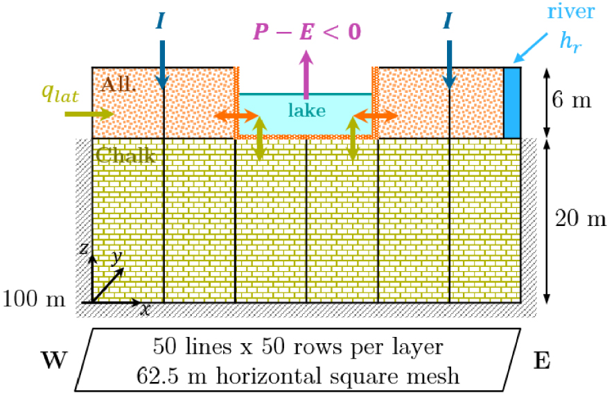
Description of the hypothetical two-layer case study.
The surface runoff is considered to be zero. The gravel pit is fed by precipitation of 675 mm/year but is subject to a higher evaporation of 710 mm/year. The same specific conductance is chosen for the bed and the banks of the gravel pit, which translates using Equation (3) into equivalent specific conductances of 4.0 × 10⁻⁵ s−1 for the vertical interfaces separating the gravel pit from the alluvial deposits and 4.5 × 10⁻⁶ s−1 for the horizontal interfaces between the lake bottom and the chalk. Multiplying by the surface area of the interface gives conductances Cn of 1.5 × 10⁻² m2⋅s−1 and 1.8 × 10⁻² m2⋅s−1 respectively.
Two simulations were carried out, in steady and transient states, using a time step of one day and the explicit procedure for the lake scheme. The threshold for groundwater convergence was set to 0.0001 m. The forcings remain constant during the transient simulation, which is initialised under arbitrary conditions but sufficiently far from the steady state, with the initial lake level at its minimum and contrasting conditions in the two aquifers. For a sufficiently long simulation, the transient solution must converge towards the simulated steady-state. The proposed setup and model parameters are summarised in Table 2.
Definition of the study area: model setup and parameters
| Alluvium (layer 1) | Chalk (layer 2) | Gravel pit (bed & banks) | River | |
|---|---|---|---|---|
| Horizontal hydraulic conductivity Kh (m⋅s−1) | 6 × 10⁻³ | 5 × 10⁻⁴ | ||
| Vertical hydraulic conductivity Kv (m⋅s−1) | 6 × 10⁻⁴ | 5 × 10⁻⁵ | ||
| Storage S (-) | 0.06 | 0.001 | ||
| Thickness e (m) | 6 | 20 | ||
| Specific conductance Cg (s−1) | 5 × 10⁻⁵ | |||
| Initial conditionsh0 (m) | 123 | 122 | 120 | 124.5 |
| Boundary conditions | ||||
| Dirichlet hr (m) | 124.5 | |||
| Neumann qlat (m3⋅s−1) | 1.85 × 10⁻³ | |||
| Recharge I (m⋅s−1) | 6.9 × 10⁻⁹ | |||
| Precipitations P (m⋅s−1) | 2.14 × 10⁻⁸ | |||
| Evaporation E (m⋅s−1) | 2.25 × 10⁻⁸ |
3.2.2. Simulation results
A first set of simulations made it possible to ensure the similarity of the results produced by the two codes CaWaQS and Modflow in the absence of a gravel pit. In steady-state, the simulated head differences over the study area are less than 1 mm and negligible in terms of calculation accuracy. The introduction of a gravel pit has an impact on the distribution of equipotential lines and therefore on the flow pattern in the vicinity of the water body, converging upstream and diverging downstream (Figure 3a). The water table is lowered upstream of the gravel pit lake up to more than 8 cm, while a high hydraulic gradient develops downstream (Figure 3b). Between the two models CaWaQS and Modflow, the simulated head differences in the alluvial aquifer do not exceed 0.1 mm, within the margin of error of the case without a gravel pit. The water budget of the gravel pit is detailed in Table 3. The atmospheric moisture deficit E − P of 35 mm⋅year−1 results in a net inflow to the gravel pit of the same magnitude, of which nearly three quarters are from the alluvial aquifer. There is no difference between the flows calculated by each code.
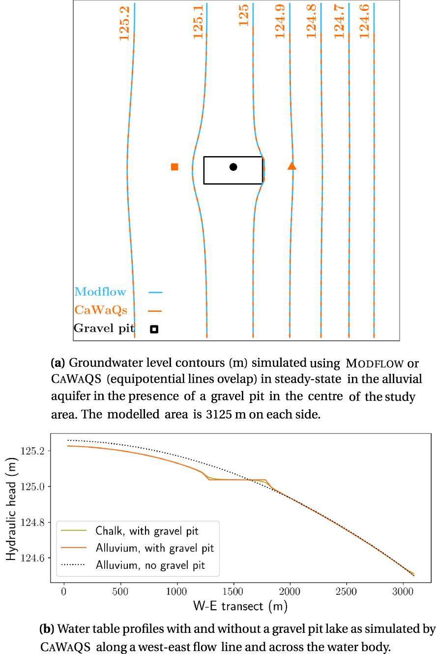
Simulation results for validation.
Gravel pit lake water balance in steady-state
| Precipitation (m3⋅day−1) | Evaporation (m3⋅day−1) | Groundwater flows (m3⋅day−1) | ||||
|---|---|---|---|---|---|---|
| Inflow | Outflow | |||||
| InV | InH | OutV | OutH | |||
| CaWaQS | 260.0 | 273.4 | 436.1 | 164.3 | 425.1 | 161.9 |
| Modflow | ||||||
V and H indicate flow through vertical interfaces between the gravel pit and the first layer and through horizontal interfaces between the gravel pit and the deeper layer, respectively.
When using the explicit procedure at a daily time step, the simulated lake level evolution was almost identical between the lake module of CaWaQS and Lak, despite some differences at the beginning of the simulation, maximum on the first day (0.1 m). By decreasing the time step from one to half and then a quarter day, the transient CaWaQS model results in a consistent lake level, whatever the time step, with a maximum difference of less than 0.5 m at the beginning of the simulation, equivalent to that obtained with Modflow (0.48 m versus 0.42 m respectively) but which lasts longer. The temporal evolution of the heads simulated by the two numerical codes is compared at a time step of 0.25 day at two points in the alluvial aquifer, upstream and downstream of the gravel pit (see location in Figure 3a), and in the gravel pit itself. Figure 4a illustrates the convergence of the water levels in the aquifer and the gravel pit lake towards their equilibrium values. For the gravel pit, the difference in lake level is maximum on the first day of simulation (0.021 m) and decreases with time (Figure 4). It is higher, although still acceptable, than that obtained at the same point in the alluvial aquifer in the absence of a gravel pit (0.002 m). Water balance calculations for the lake show a similar evolution of the inflow and outflow of the gravel pit from one code to another (Figure 5). After an initial filling phase, the lake acts as a flow-through system, with the rate of groundwater inflow nevertheless always exceeding the outflow (see steady-state water balance in Table 3).
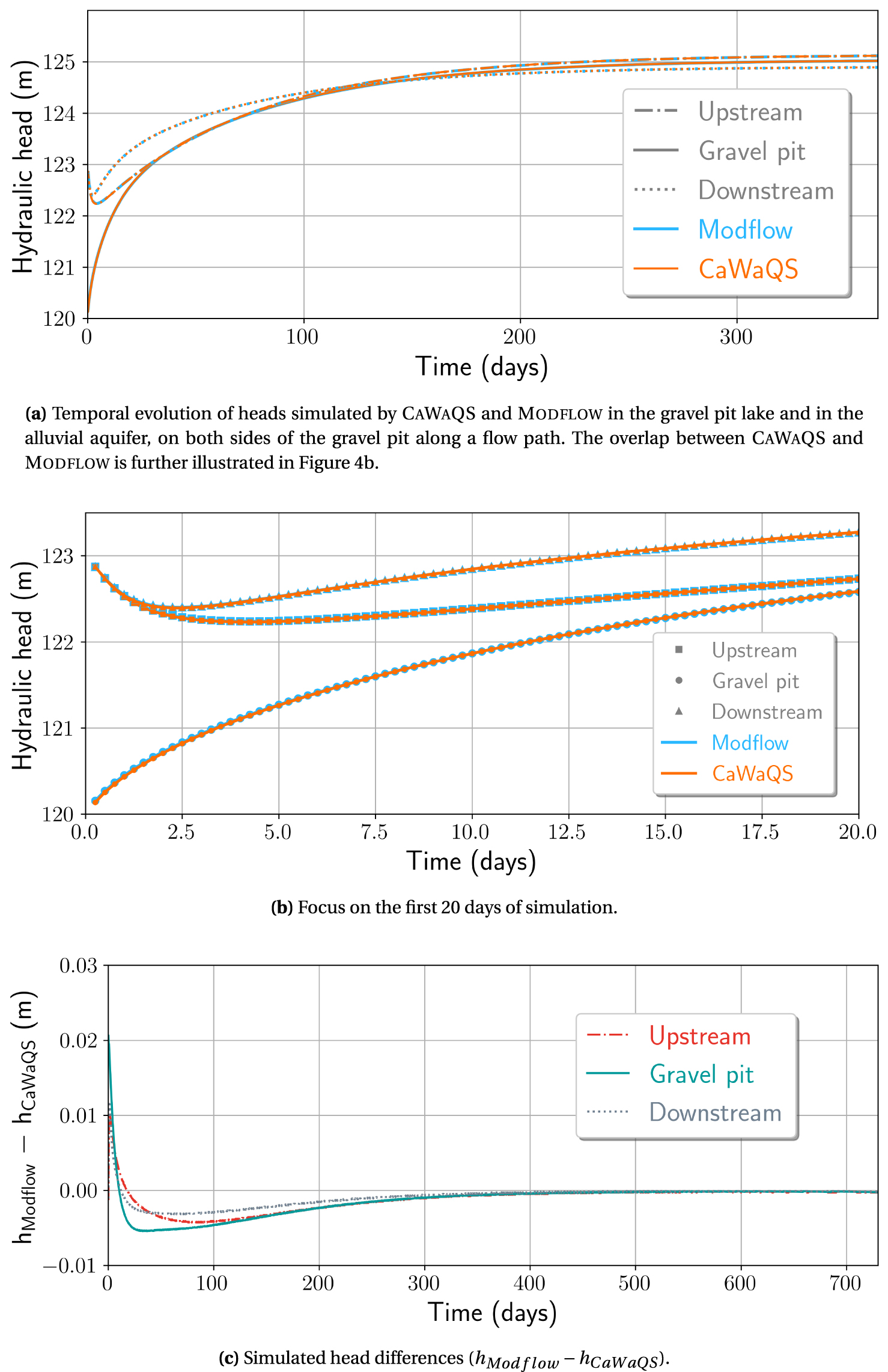
Detailed comparison CaWaQS–Modflow at three points (see location in Figure 3a) under transient conditions (explicit scheme, 0.25 day time step).
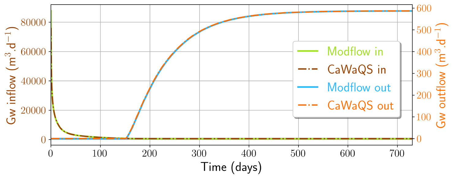
Flows into and out of the gravel pit lake during the transient run, as simulated by the two codes.
Thus validated and operational, the lake module has been integrated into the modelling platform as a specific library, which can be activated if needed. The test case configuration was taken as the baseline model for further sensitivity analysis to explore the impact of the introduction of a gravel pit lake on the behaviour of a hydrogeological system composed of two connected aquifers in interaction with a river.
4. Numerical experiments characterising gravel pit lake–aquifer interactions
In a third step, in silico experiments are run to illustrate the general principles governing the interactions between a gravel pit lake and the aquifer system in which it is embedded, principles which were recalled in the first part of the present work. The modelling approach offers the possibility of quantifying the exchange flows between the gravel pit and the aquifers and of simulating the changes in lake level and water table following gravel excavation. We first simulate the gravel pit lake–groundwater system under steady-state conditions. By varying the various parameters that could impact groundwater seepage to the lake and local water levels, we analyse their relative significance. We then examine the response of the gravel pit lake to cyclic transient boundary conditions, whose influence on the seasonal water balance terms is also investigated.
4.1. Simulations design
Steady-state simulations were carried out from the base case (#1) using various configurations relative to (i) geometrical factors (#2 to #8): size, shape and depth of the gravel pit lake, number of lakes, lake orientation with respect to the direction of flow, distance of the gravel pit from the river, (ii) hydrodynamical factors (#9 to #15): hydraulic conductivity contrasts within the groundwater system, ratio of horizontal to vertical hydraulic conductivity and clogging of the lake bed and banks, and (iii) meteorological factors (#16 to #19): groundwater recharge (I and qlat) and atmospheric moisture deficit (E − P). The values of the parameters chosen for the tests are shown in Table 4. Although hypothetical settings are simulated, it is expected that these values and the selected magnitude in their change from the baseline conditions are realistic and representative of gravel pit lake environments.
Design of the steady-state simulations: model parameters
| Simulations | Geometrical factors | |||||
|---|---|---|---|---|---|---|
| Size (m2) | Shape | Depth (m) | Number | Orientation | Position | |
| #1 ref. | 140,625 | Rectangular | 6 | 1 | Parallel | Central |
| #2 size | 257,812.5 | |||||
| #3 square | Square | |||||
| #4 depth | 20 | |||||
| #5 × 3 | 46,875 | 3 | Perpendicular | |||
| #6 ppdcl | Perpendicular | |||||
| #7 up | Upstream | |||||
| #8 down | Downstream | |||||
| Hydrodynamical factors | ||||||
| Transmissivity T (m2⋅s−1) | Anisotropy Kv∕Kh | Clogging Cg (s−1) | ||||
| Alluvium | Chalk | |||||
| #1 ref. | 3.6 × 10⁻² | 10−2 | 0.1 | 5 × 10⁻⁵ | ||
| #9 homo | 3.6 × 10⁻² | 1 | Bed | 5.09 × 10⁻⁵ | ||
| #10 Tall | 3.6 × 10⁻¹ | |||||
| #11 Tch | 10−4 | |||||
| #12 𝛼 | 0.5 | |||||
| #13 noC | No clogging | |||||
| #14 C4 | All but upstream | 10−8 | ||||
| #15 Ctot | All banks & bed | 10−8 | ||||
| Meteorological factors | ||||||
| qlat (m3⋅s−1) | I (m⋅s−1)/(mm⋅year−1) | P − E (m⋅s−1)/(mm⋅year−1) | ||||
| #1 ref. | 1.85 × 10⁻³ | 6.9 × 10⁻⁹ ∕ 218 | − 1.1 × 10⁻⁹ ∕ −35 | |||
| #16 E+ | − 1.38 × 10⁻⁸ ∕ −44 | |||||
| #17 P | 1.1 × 10⁻⁹ ∕ 35 | |||||
| #18 P+ | 1.38 × 10−8 = 2 × I#1 / 44 | |||||
| #19 q+ | 6.51 × 10−2 = I#1 | 1.96 × 10−10 = qlat #1 / 6 | ||||
Two sets of transient simulations are used, one involving a step change in water inflow and the other a sinusoidal variation in its boundary conditions. The first set, based on all the simulations carried out in steady-state and defined as initial conditions, consists of cancelling all the recharge terms of the lake–groundwater system (qlat, I and P − E) and following the rate of gravel pit lake level recession until a new equilibrium is approached. The response time 𝜏c of the gravel pit lake is then deduced. This characteristic time is given by the exponential decay constant, adjusted between 10 and 90% of the total lake level change due to the cessation of recharge, in order to take into account the time necessary for the system to reach a purely exponential decay [Cuthbert 2014]. A value of 0.06 is assigned to the storage coefficient of the upper aquifer and of 0.001 for the lower aquifer, resulting in hydraulic diffusivity T∕S of 0.6 and 10 m2⋅s−1, respectively.
Additional transient simulations are developed to examine the response of the groundwater–lake system to periodically oscillating recharge (I and P − E) and boundary conditions (qlat, hr), independently at first and then by applying all the forcings simultaneously. The sinusoidal input signal is expressed in the form of a cos(𝜔t), where a is the driving force amplitude (L, L⋅T−1 or L3⋅T−1), 𝜔 = 2π∕To is the oscillation frequency (T−1), To is the oscillation period (T) and t is the time (T). At the river boundary, the head amplitude is about 0.3 m. In this scenario, mean driving forces were applied so that qlat = I = 2.23 × 10⁻² m3⋅s−1 and I = E − P = 2.36 × 10⁻⁹ m⋅s−1. The period is 1 year, i.e., seasonal variations are investigated. The resulting cyclic stresses are illustrated in Figure 7. Steady-state groundwater heads and lake level are used as initial conditions and the transient model is run with daily time steps until a quasi-steady oscillatory state is reached. Models are used to evaluate the response of the gravel pit lake’s level to periodically changing hydraulic conditions, for different configurations involving increasing clogging of the lake (ref., C4 and Ctot).
4.2. Simulation results
4.2.1. Steady-state analysis
The hydrodynamic disturbance caused by the gravel pit lake, as simulated by the gravel pit lake–aquifer system models, is assessed using several criteria (see Table 5) that measure (i) the impacts in terms of groundwater and lake levels, as compared to equivalent baseline simulations with no gravel pit: to this end, we calculate the difference in water levels and the position of the Kippungslinie (𝜅); (ii) changes in the water budget components, (iii) the water residence time of the gravel pit lake.
Main results of the steady-state and transient simulations: water levels and balance components
| Simulations | Water levels | Water balance | |||||||||
|---|---|---|---|---|---|---|---|---|---|---|---|
| 𝛥h− (m) | 𝛥h+ (m) | hL (m) | 𝜅 (%) | 𝜏c (days) | Qin | E∕(Qin+P) (%) | InV (%) | InH (%) | 𝜏r (years) | ||
| (m3⋅day−1) | (%) | ||||||||||
| #1 ref. | −0.084 | 0.038 | 125.037 | 70 | 73 | 600 | 10 | 32 | 73 | 27 | 3.2 |
| #2 size | −0.116 | 0.035 | 125.017 | 77 | 84 | 851 | 15 | 38 | 72 | 28 | 4.2 |
| #3 square | −0.059 | 0.019 | 125.035 | 73 | 74 | 569 | 10 | 33 | 73 | 27 | 3.4 |
| #4 depth | −0.088 | 0.033 | 125.033 | 73 | 71 | 738 | 13 | 27 | 84 | 16 | 2.6 |
| #5 × 3 | −0.032 | 0.004 | 125.048 | 75 | 74 | 729 | 13 | 28 | 79 | 21 | 2.7 |
| #6 ppdcl | −0.040 | 0.004 | 125.054 | 80 | 75 | 590 | 10 | 32 | 74 | 26 | 3.3 |
| #7 up | −0.050 | 0 | 125.201 | Ø | 85 | 225 | 4 | 56 | 73 | 27 | 8.9 |
| #8 down | −0.122 | 0.074 | 124.718 | 63 | 60 | 988 | 17 | 22 | 73 | 27 | 1.8 |
| #9 homo | −0.055 | 0.023 | 124.841 | 71 | 78 | 661 | 11 | 30 | 35 | 65 | 2.8 |
| #10 Tall | −0.009 | 0.006 | 124.568 | 62 | 10 | 180 | 3 | 62 | 78 | 22 | 9.9 |
| #11 Tch | −0.106 | 0.049 | 125.182 | 69 | 94 | 583 | 10 | 32 | 100 | 0 | 3.4 |
| #12 𝛼 | −0.084 | 0.037 | 125.034 | 70 | 71 | 627 | 11 | 31 | 65 | 35 | 3.1 |
| #13 noC | −0.091 | 0.031 | 125.029 | 75 | 70 | 840 | 15 | 25 | 90 | 10 | 2.3 |
| #14 C4 | −0.038 | 0.143 | 125.143 | 103 | 102 | 25 | <1 | 96 | 100 | 0 | 79.7 |
| #15 Ctot | −0.171 | 0.019 | 124.950 | −4 | 1110 | 13 | <1 | 100 | 7 | 93 | 142.6 |
| #16 E+ | −0.110 | 0.011 | 125.011 | 87 | 73 | 667 | 12 | 35 | 72 | 28 | 2.9 |
| #17 P | −0.079 | 0.042 | 125.042 | 66 | 73 | 589 | 10 | 30 | 73 | 27 | 3.3 |
| #18 P+ | −0.053 | 0.069 | 125.068 | 47 | 73 | 524 | 9 | 28 | 73 | 27 | 3.7 |
| #19 q+ | −0.134 | 0.095 | 125.205 | 58 | 73 | 1138 | 20 | 20 | 73 | 27 | 1.8 |
𝛥h− and 𝛥h+ are respectively the maximal fall and rise in water levels along a flow path across the gravel pit lake, compared to the equivalent case without a lake, hL is the simulated gravel pit lake level, 𝜅 is the position of the Kippungslinie within the lake as counted from upstream, 𝜏c is the response time of the gravel pit lake, Qin is the groundwater inflow to the gravel pit lake, also expressed as a percentage of total flow in the aquifer system, E∕(Qin + P) is the fraction of precipitated water and inflowing groundwater evaporated from the gravel pit lake, InV and InH are inflows through vertical interfaces between the gravel pit and the alluvial layer and through horizontal interfaces between the gravel pit and the chalk layer, respectively, here expressed as a percentage of total inflow Qin, and 𝜏r is the water residence time of the gravel pit lake. Numbers in bold are discussed more specifically in the text.
For the reference simulation #1, the steady-state model results in a gravel pit lake level of 125.037 m, a level that corresponds to the pre-extraction water table established at a distance of 70% of its size from its upstream side. For an unclogged gravel pit lake, it moves not at mid-point of the gravel pit lake [Wilson 1984] but downward at 75%. This is in line with the parabolic water table profile, here related to the specified recharge and which should apply further in the case of an unconfined shallow aquifer. The position of the Kippungslinie therefore reflects not only the presence and extent of the lake sealing as expected [Wilson 1984, simulations #14 and #15] but also the recharge conditions of the system (see simulations #16, #18 and #19). A positive atmospheric lake balance (#18) equilibrates the lake at mid-point while as the E − P deficit increases, so decreases the predicted level of the gravel pit lake (#16, Figure 6a), as well as the water table downstream of the lake. The main changes in lake water levels are nonetheless predicted as a consequence of lake sealing. While the two simulated water table profiles in the case of clogged lake (#14 and #15) are similar, characterised by slight rise and fall respectively upstream and downstream of the lake, e.g., a limited impact on alluvial groundwater levels, the predicted lake levels are opposite. A partially clogged lake gives rise to a high lake level (125.143 m), as often described in the literature [e.g., Peaudecerf 1975] and acts as a reservoir fed by the alluvial aquifer upstream (100% of inflowing groundwater) and mainly drained by the chalk aquifer. In contrast, if totally sealed, the gravel pit lake ends as a terminal lake, with a low level (124.950 m), nearly 20 cm lower, mainly fed by the deep aquifer and where groundwater inflow exactly compensates for the atmospheric moisture deficit. A high hydraulic head gradient, of 3.3‰, i.e., more than ten times greater than the initial gradient, is found upstream of the excavation, as opposed to its downstream location in C4 simulation. The hydraulic gradients on either side of the lake are all the more pronounced as the clogging is significant. In the absence of clogging, the transition between the gravel pit lake and the water table is smoothed. In this case, the simulated water table is similar to that obtained from an additional run using the “high K” technique (referred to as #13b in Figure 6a).
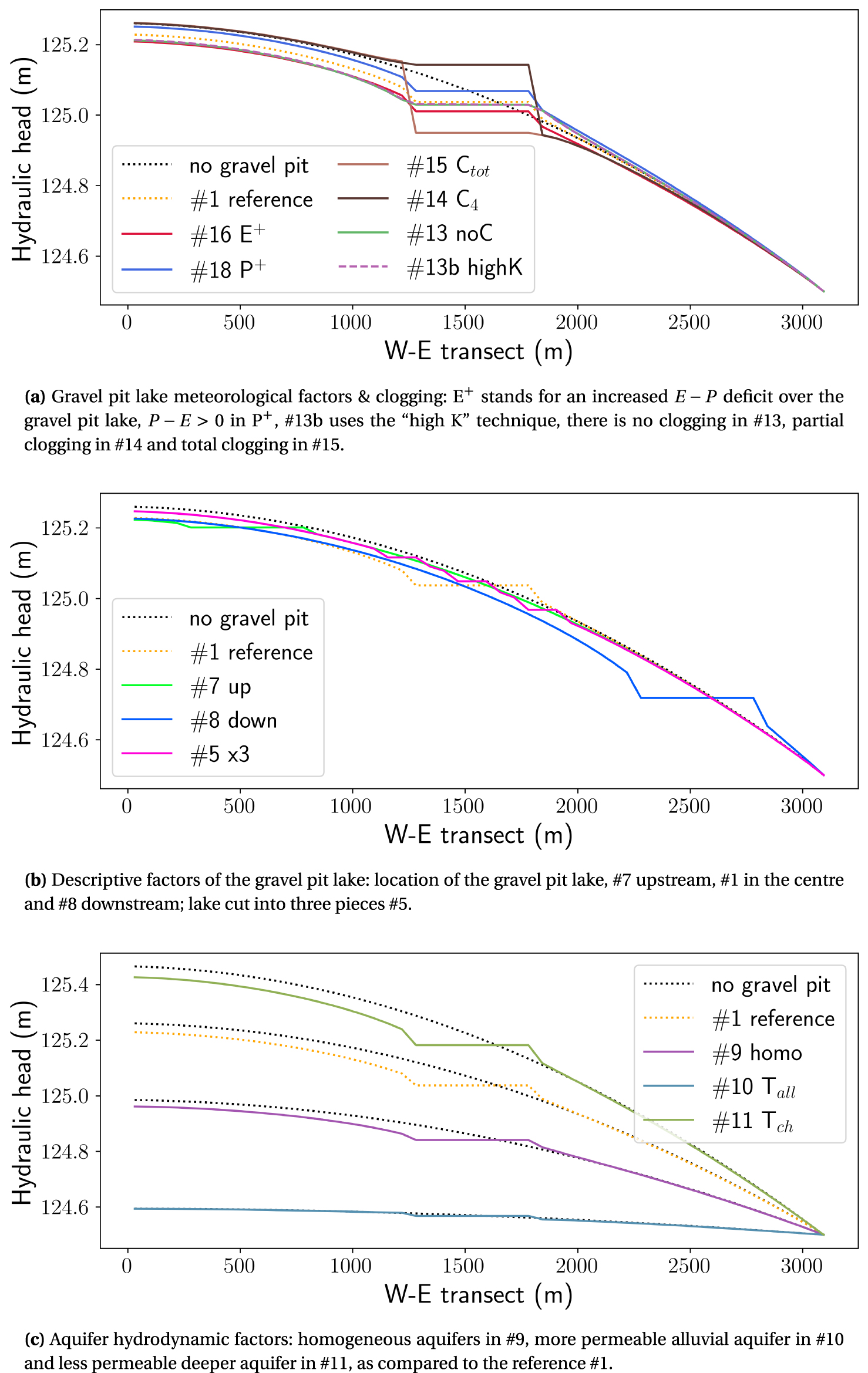
Selected results of the steady-state simulations along a west–east flow line and across the water body, for different configurations of the gravel pit (see location in Figure 3a).
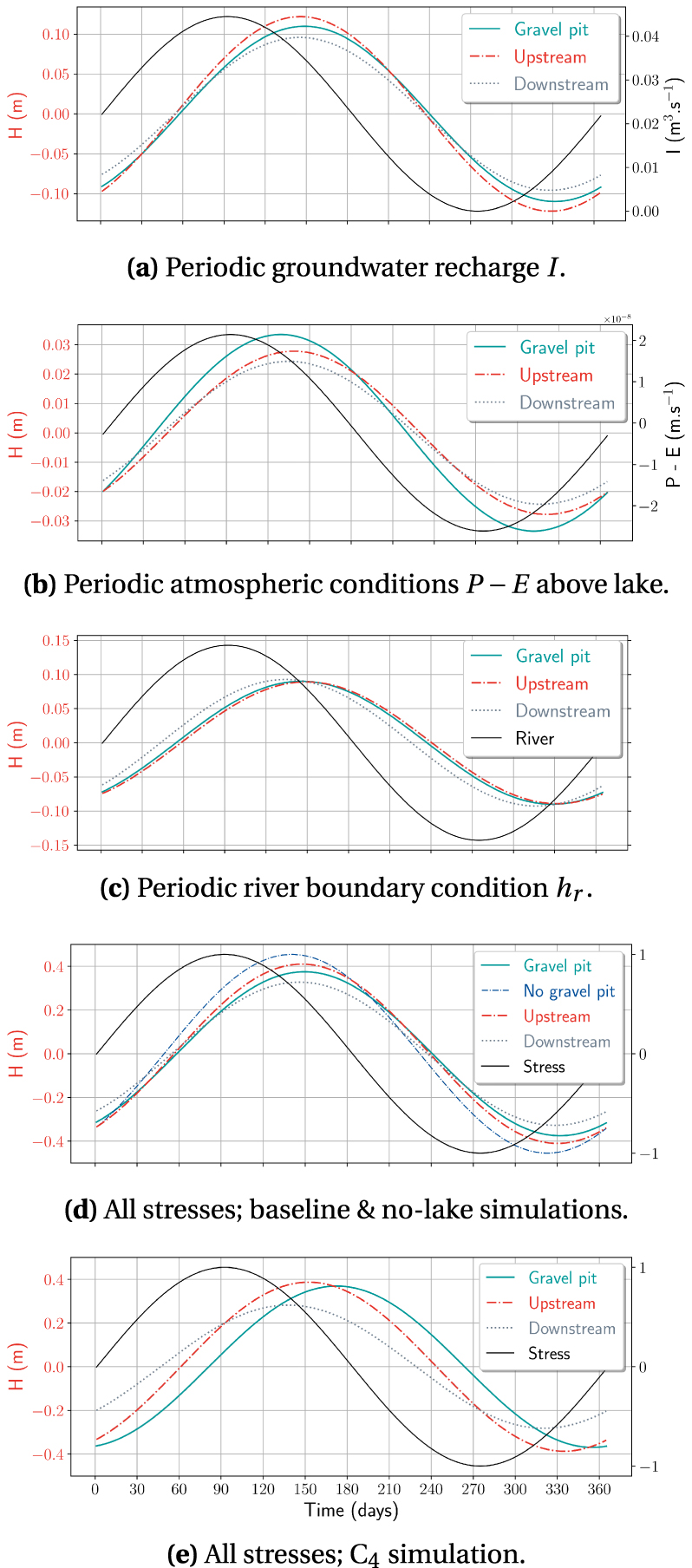
Theoretical response of the gravel pit lake level, and of selected upstream and downstream water levels in the alluvial aquifer (see location in Figure 3a), here represented by their amplitude, to various simple sinusoidal hydraulic stresses applied to the lake and the aquifer (shown in black in the figure). Results correspond to baseline simulation, except (e), for a partially clogged gravel pit lake (C4 simulation). Also plotted in (d), the equivalent upstream groundwater level simulated in the absence of a gravel pit. The graphs share a common x-axis. Masquer
Theoretical response of the gravel pit lake level, and of selected upstream and downstream water levels in the alluvial aquifer (see location in Figure 3a), here represented by their amplitude, to various simple sinusoidal hydraulic stresses applied to the lake ... Lire la suite
In the chosen configuration, with a Dirichlet boundary condition downstream and a Neumann boundary condition upstream, the impact of the gravel pit lake on groundwater levels is mainly felt upstream, where the water table is generally lowered as compared to the pre-extraction levels, whereas the lake influence is rather limited downstream of the gravel pit lake (Figure 6). The intensity of the response of the aquifer system to the creation of the water body is also conditioned by the position of the lake along the flow line. Far from the low points of the valley, only a limited drop in the water table is simulated (#7, Figure 6b). It is even more pronounced the closer the gravel pit lake is to the river (#8), where the initial water table gradient is higher. This is also the case when the transmissivity of the system decreases (#11, for the chalk aquifer, Figure 6c). On the other hand, in a highly permeable aquifer (#10, for the alluvial aquifer), the change in water table from the pre-extraction situation will be difficult to measure (see Table 5). The impact of the gravel pit on groundwater levels can finally be reduced by choosing a gravel pit layout perpendicular to the flow, which offers a larger exchange surface to the flow (#6 and #3), by favouring the number of water bodies (#5, Figure 6b) rather than a single large lake (#2), whose level could end up higher than the natural ground level downstream.
With regards to the water balance, groundwater exchange with the gravel pit lake represents, in the examples considered here, up to 20% of the total flow circulating in the aquifer system. It is enhanced when a higher upstream groundwater flow is intercepted by the water body (#19 and #8), especially if the gravel pit is larger or deeper (#2 and #4), and it is generally accompanied by a decrease in inflowing water evaporated from the lake. A greater number of water bodies also means an increased rate of water cycling (#5). Two parameters of the model again play a major role in controlling the lake seepage, namely the bed and banks conductance (#14 and #15) and the hydraulic conductivity of the superficial aquifer (#10). Indeed, the rate of groundwater input to the lake becomes a negligible component of the overall water balance when clogging is severe. With respect to the hydraulic conductivity of the alluvial aquifer, the model results indicate that there is a reduction in groundwater inflow to the lake, which is related to the lower hydraulic gradient, while the conductance of the lake/aquifer interface remains dominated by bank clogging.
For an isotropic and homogeneous porous media (#9), upward flux of deep groundwater into the gravel pit lake is predominant due to the larger area offered to the flow by the bottom of the gravel pit. However, if the medium is anisotropic and the hydraulic conductivity decreases with depth, results show that the majority (three quarters in the reference case) of the lake inseepage comes from the shallow aquifer (horizontal conductance of the interfaces one order of magnitude higher than the vertical conductance in simulation #1). The share of flow through the lake bottom may increase in case of clogging if it is homogeneous (see noC, ref. and Ctot simulations). The relative contributions of the two aquifers are indeed variable and depend on the hydraulic conductivity contrast between the two units (#9–11), the ratio of horizontal to vertical hydraulic conductivity (#12) and the extent of lake sealing (#13–15). They are highly dependent on local groundwater flow conditions, according to whether the gravel pit is complete and rests on a low permeability layer (no exchange via the bottom of the gravel pit in the case tested here, #11), on the vertical heterogeneity of the bank clogging, or on whether the banks are more clogged than the bottom of the gravel pit due to the partial backfilling of the excavation with the overburden.
The computation of the water residence time 𝜏r in the gravel pit lake summarises the previous observations concerning the level at which the gravel pit lake equilibrates and its exchanges with the aquifers. In this theoretical case study, the water retention time is around 3 years. In particular, it is variable along a flow path, here five times higher upstream than downstream (down versus up simulations). It becomes longer as the amount of seepage is reduced (e.g., Tall simulation), mainly with the ageing of the gravel pit and the subsequent clogging (residence time more than one order of magnitude higher than the median).
4.2.2. Transient analysis
The transient numerical models are used to investigate the dynamic changes in gravel pit lake water level as a result of variations in the balance between inputs and outputs of water. Estimating gravel pit lake response times provides information on the time required for the lake level to adjust to these changes. They are shown in Table 5 for each of the 19 cases. The calculated 𝜏c values range from 2 to 3 months. It is dependent on the horizontal distance away from the divide, and is longer for the lake in the most upgradient position. The lake response is also defined by the size of the gravel pit. The results mainly illustrate how the response for any gravel pit lake is determined by the hydrodynamics properties of the lake–groundwater system. The larger the hydraulic diffusivity of the shallow aquifer, the shorter the time to reach the equilibrium lake level and conversely when the gravel pit lies on a low permeability bedrock. Finally, 𝜏c depends largely on the connectivity between the gravel pit lake and groundwater, i.e., on the conductance of their interfaces. Significantly slower responses, up to 3 years, are simulated as a result of sealing of the bed and banks of the gravel pit lake.
For small lakes such as those in gravel pits, however, relatively short response times are expected and hence an ability to propagate forcings whose period of fluctuations is of the same order as the response time, i.e., also short. In this theoretical case study, the annual period is close to 2π𝜏c. For lower frequency components, the gravel pit lake will remain approximately in equilibrium while high frequency signals will be attenuated independently of 𝜏c, the lake acting as a low pass filter [Mason et al. 1994].
We now examine the one-year response of the gravel pit lake to such periodic forcing, once the lake level has reached a pseudo-sinusoidal steady-state. Figure 7 illustrates the rise and fall of water levels around the average in the gravel pit lake and in the shallow aquifer about 100 m upstream and downstream of the lake, in response to seasonal varying groundwater (Figure 7a for I; not shown for recharge flux qlat across the lateral boundary) and lake recharge (Figure 7b), river head (Figure 7c) and to all hydraulic stresses considered together (Figure 7d), for the base case. Water table fluctuations are greater near the groundwater divide than in the discharge area, except where changes in the river level are the main driver, for example during high-flow periods. Their simulated amplitude H and phase 𝜙 values are summarised in Table 6. Relative to the no-lake case, the results show that the presence of the gravel pit lake dampens the groundwater wave propagation, as the water table exhibits smaller amplitude and increased phase lag (see also Figure 7d), underlining the dominant role of the storage effect of the lake, as pointed out by Jazayeri et al. [2021]. Regarding the gravel pit lake’s level itself, slower readjustments also occur in response to the sinusoidal variation in groundwater recharge, as compared to the aquifer, to be related to the response time 𝜏c of the gravel pit lake. The influence of the varying precipitation inputs and evaporation outputs into/from the lake is felt beyond its physical extent on either side of the lake, as illustrated in plot Figure 7b, but is expected to be of limited extent, due to the small amplitude involved, and masked by the variability of groundwater seepage (Figure 7d).
Results of the baseline transient simulations under the action of each stress separately and then all together: amplitude H and phase shift 𝜙 of the gravel pit lake level and of the alluvial groundwater level at about 100 m upstream and downstream of the lake
| Stress | Upstream | Gravel pit lake | Downstream | |||
|---|---|---|---|---|---|---|
| H (m) | 𝜙 (days) | H (m) | 𝜙 (days) | H (m) | 𝜙 (days) | |
| I | 0.122 | 52 | 0.110 | 56 | 0.096 | 51 |
| qlat | 0.172 | 56 | 0.145 | 65 | 0.120 | 65 |
| hr | 0.089 | 56 | 0.090 | 53 | 0.093 | 40 |
| P − E | 0.028 | 42 | 0.033 | 36 | 0.024 | 38 |
| All | 0.410 | 55 | 0.375 | 58 | 0.328 | 53 |
| No gravel pit | 0.455 | 48 | — | — | 0.336 | 44 |
| All C4 | 0.387 | 60 | 0.370 | 80 | 0.282 | 46 |
| All Ctot | 0.369 | 44 | 0.130 | 91 | 0.216 | 46 |
Also presented are the results of an equivalent simulation with no gravel pit lake, in response to the periodic variations of the first three hydraulic stresses, and two additional simulations involving respectively a partially and a totally clogged gravel pit lake.
How the sealing layer on the banks and at the bottom of the lake influences the attenuation and phase shift of the input signal within the lake–aquifer system is illustrated using the cases of a partially and a totally clogged gravel pits (C4 and Ctot). Due to the longer response time of the water-filled pit, a further attenuation in amplitude and a significant shift in phase (from 58 to 81 or even 91 days) of the lake’s response are simulated (shown for C4 case in Figure 7e), while contrasting effects on signal propagation are noted when comparing upstream and downstream of the alluvial aquifer on either side of the lake.
The water regime of the gravel pit lake is not only the result of precipitation inputs exceeding evaporation outputs or vice versa but is mainly determined by the seasonal variability of net groundwater flow Qin − Qout. Assessing groundwater–lake exchanges is therefore a key element in the overall understanding of gravel pit lake hydrology. The simulated seasonal distribution of the lake water balance components over a hydrological year supposed to start in October is presented in Figure 8, where positive values indicate fluxes recharging the pit lake. During the wet season, water storage in the lake is provided by net influx of groundwater and direct precipitations, in proportions that will depend on local climate, hydrogeological conditions and gravel pit lake hydraulic properties. During the dry season, the surface water evaporation is mainly compensated by the release of water stored during the preceding high-flow period, with an additional groundwater supply, at the end of the dry period in the baseline case or in the case of a completely clogged gravel pit (C4).
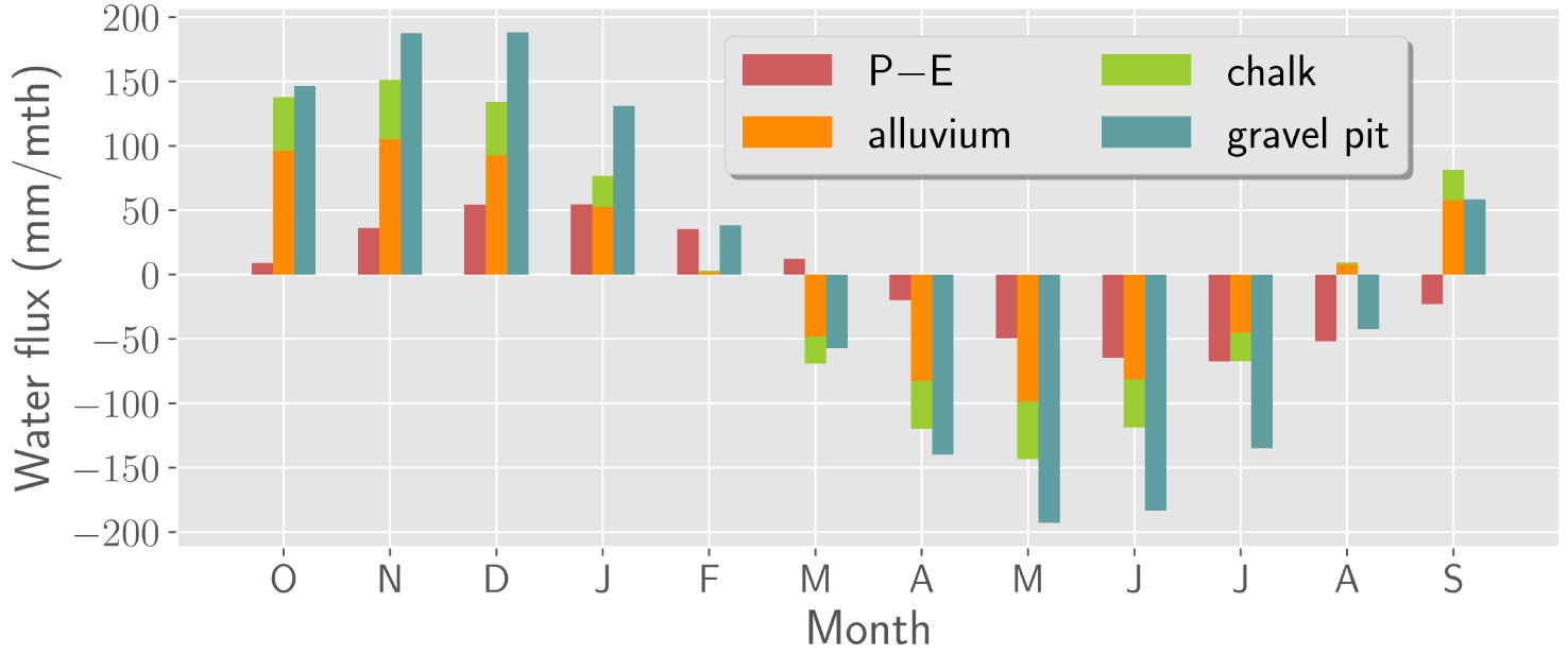
Water balance of the gravel pit lake: the monthly averages of net atmospheric inputs (P − E), net seepage from the alluvial and chalk aquifers (Qin − Qout), and variations in the gravel pit storage are shown for the reference transient simulation, under the effect of all applied stresses.
5. Conclusion
The theoretical numerical case studies, conducted in this work under steady-state and transient regimes for a single gravel pit lake, illustrate the diversity of the situations that can be encountered under real-world conditions. They are useful for understanding the mechanisms that govern the temporal and spatial occurrence of groundwater-gravel pit lake interactions. The intensity of their exchanges is one of the particularities of these man-made lakes, which distinguishes them from natural lakes, although the importance of this process is increasingly recognised even for the latter [e.g., Hokanson et al. 2022]. The gravel pit lake water level and its changes are primarily dependent on the variability of the groundwater contribution, while the balance between precipitation and evaporation plays a secondary role. The significant amount of groundwater through-flow, combined with the small size of the open pits, results in short residence times. Low values, ranging from a few days to one and a half years, are indeed generally compiled for gravel pits [Schanen 1998; Weilhartner et al. 2012]. This has implications for the nutrient budget of the gravel pit lake and hence, their ecology and the effective management of these aquatic ecosystems. Accurate spatial and temporal quantification of groundwater inflow and outflow to the lake is a prerequisite for estimating the mass balance of its dissolved components.
Despite the interannual variability due to surface water evaporation is generally outweighed by the through-flow of groundwater, it is still a potential sink term for the aquifer system. More investigation is needed to obtain valid estimations of the magnitude and seasonal distribution of open water evaporation in the particular case of gravel pit lakes. In this respect, state-of-the-art thermodynamic lake models [Ottlé et al. 2020] or isotope mass balance models [Gibson 2002] should prove useful in estimating the evaporation losses. A generalisation of studies on gravel pit lakes to any type of climatic context is also awaited, as well as a broad assessment of how groundwater-gravel pit lake interactions may be modified as a result of climate change, following the pioneer work of Mollema and Antonellini [2016]. Given their small size, it is expected that gravel pit lakes will have a more sensitive short-term response to seasonal events than to low-frequency climatic events such as droughts, but this needs to be checked against the geographical context of each site.
Assessing the response of the gravel pit lake–aquifer system to changes in climate conditions and land use may require further modelling developments to take into account a wider range of processes such as a more comprehensive description of vertical flows in the vadose zone, whether to better estimate infiltration and evapotranspiration processes or additional delays in water transfer to the aquifer. Also, there is less understanding of how extreme events, such as flash floods or droughts, may influence this behaviour [Cross et al. 2014] and additional coupling of the subsurface to the surface would be useful in this respect. This is indeed one of the limitations of the simple modelling approach we have developed within the CaWaQS platform, as well as the simplification of solving the flow equation only for a confined aquifer for the moment. In this latter case, this leads in particular to a slight overestimation of the flows exchanged with the shallow aquifer (of the order of +5%) at the expense of the deep aquifer (−10%), as compared to the results of an additional baseline run carried out using Lak-Modflow in unconfined mode. Greater numerical stability and ease of deployment at the scale of a real case study with multiple water bodies are however expected.
The next step is to use this mathematical tool for modelling purposes in such a regional case study. Although gravel pit lakes are becoming an increasingly common type of freshwater and their local impacts are regularly examined, they are more rarely studied on a regional scale. To fill this gap, we are currently developing an application in the alluvial plain of the Seine River, upstream of Paris. In the so-called Bassée region, a thousand small water bodies resulting from post-war sand and gravel extraction are scattered across the floodplain. The existence of numerous water level records on well-maintained sites, future accurate remote sensing of their temporal variations by the SWOT satellite, and the present numerical code will be of great benefit in deciphering the cumulative effect of a multitude of gravel pits of different shape and size in a heterogeneous hydrogeological environment. Such a combination of tools will also be useful in monitoring water resources in strategic areas where water and aggregate resources coexist.
Conflicts of interest
The authors declare no competing financial interest.
Dedication
The manuscript was written by AJ. SW developed the first version of the code and TV updated it, under the supervision of AJ. FC participated in the sensitivity analysis conducted by AJ. NF provided access to CaWaQS and expertise. All authors have given approval to the final version of the manuscript.
Acknowledgements
This work was funded by the Centre National d’Etudes Spatiales (CNES) through the TOSCA-SPAWET programme, with additional support from the PIREN-Seine programme. The authors warmly thank the two referees whose valuable comments helped to clarify the manuscript.