


 CC-BY 4.0
1. Introduction
In a global energy transition context, the potential of geothermal power, i.e. electricity generation from geothermal energy, might be underestimated. The installed capacity of geothermal power plants has increased by 27% between 2015 and 2020 [Huttrer 2021]. The world’s total geothermal power reached 15.9 GWe (electric gigawatt) in May 2020 and the regular increase since 2010 would imply a total world installed capacity of around 20 GWe (the equivalent of the average power of 20 nuclear reactors) in 2025 [Huttrer 2021]. However, this prediction is based on present-day geological models of geothermal reservoirs, which are generally assumed to be located in specific tectonic and geodynamic contexts (e.g. extensional tectonics or volcanic areas). The three main countries where geothermal exploration has recently increased are Indonesia, Kenya, and Turkey. In these and other countries where geothermal energy is exploited, surface manifestations such as geysers, hot springs, or fumaroles are observed and represent direct evidence of an underlying geothermal reservoir (e.g., Larderello, Italy; Wairakei, New Zealand; The Geysers, California; Olkaria, Kenya; Germencik, Turkey). However, in this study, we focus on specific geological systems that may host geothermal reservoirs without showing surface evidence. Permeable structures such as crustal fault zones (fault cores and hundreds of meters wide networks of interconnected fractures in the damage zone) are particularly discussed. These structures may represent unconventional geothermal resources for power production [Duwiquet 2022], since reservoir permeability would be sufficiently favorable to avoid stimulation [see Jolie et al. 2021 for a detailed review of conventional and unconventional geothermal resources].
In the following, a “high-temperature” geothermal system refers to a geothermal reservoir where the temperature is greater than 150 °C. Various definitions are used in the literature [e.g., Jolie et al. 2021] and our choice corresponds to a threshold value of temperature where exploration of such systems in France has to be officially declared. Actually, Lund et al. [2022] emphasized that electric power can be generated from geothermal systems where the temperature is as low as 90 °C, but our study will be focused on higher-temperature geothermal systems with better energy performance.
Several high-temperature geothermal systems at exploitable depths (1–4 km) do not exhibit surface manifestations (e.g., Landau in the Upper Rhine graben). Actually, “blind” or “hidden” geothermal systems were discovered accidentally during oil, gas, or mining activities [e.g., the geothermal reservoirs in the Imperial Valley of southern California, or those in the Basin and Range province; Faulds and Hinz 2015; Garg et al. 2010; Dobson 2016]. Likewise, the Soultz-sous-Forêts thermal anomaly (Upper Rhine graben, France) was first evidenced by temperature measurements performed in petroleum boreholes [Haas and Hoffmann 1929]. Recently, a blind geothermal system in western Nevada has been discovered through a “geothermal play fairway analysis”, where gravity, magnetics, resistivity, and geothermometry data were combined before deciding to drill temperature-gradient boreholes [Craig et al. 2021]. Interestingly, their predicted geothermal power reaches 16 MWe. From this example and many others, one can infer that the presence of a magmatic activity is not a prerequisite for the formation of shallow thermal anomalies. To summarize, exploitable thermal anomalies at shallow depths are probably much more present than previously assumed.
Promising areas where geothermal systems could be exploited can also be inferred from the presence of anomalously high subsurface temperature gradients. However, direct measurements of underground temperatures depend on the availability of sufficiently deep (hundreds to thousands of meters) and open boreholes. When such temperature measurements are available, downward extrapolation to greater depths may however be biased by several physical and geological processes, as detailed later. When heat flow or underground temperature data are not available, geothermal potential becomes difficult to assess, except if multidisciplinary studies are conducted [Craig et al. 2021].
However, it is well known that temperature is not the only fundamental parameter to make an exploitable geothermal reservoir. Permeability and flow rate are essential. In a sense, the role of permeability was neglected in the last decades, and artificial techniques were developed to enhance the efficiency of fluid circulation (the “Enhanced Geothermal Systems (EGS)” concept). Yet, instead of looking for anomalously hot areas where permeability could be enhanced, it might be worth searching for anomalously permeable zones, such as crustal fault zones [Bellanger et al. 2016; Duwiquet et al. 2019, 2021] where deep hot fluids would naturally rise to shallow crustal levels. This concept, which prioritizes permeable zones instead of hot zones, may strongly increase the number of favorable geological systems where blind geothermal reservoirs would be present. We therefore focus our study on hydraulically active parts of fault zones, which are recognized as preferential pathways for fluid flow.
The main objective of this study consists in opening different ways of thinking and exploring geothermal energy. More precisely, this study is aimed at (i) describing the various physical processes at the origin of the formation of geothermal reservoirs; (ii) suggesting new perspectives for geothermal exploration through different views of high-temperature geothermal systems; (iii) estimating possible targets in fault zones for the development of geothermal energy in Europe in the next decades. After describing several mechanisms at the origin of thermal anomalies in the shallow crust (Section 2), we present tectonic and geodynamic processes that can affect the thermal regime of the crust at different scales (in space and time), from mantle to crustal units (Section 3). Then a literature review focuses on crustal permeability (Section 4) and highlights the role of damage zone geometry on the heat transport mechanisms and on the conditions for the onset of buoyancy-driven convection (Section 5). We discuss the role of tectonic regimes in the establishment of thermal anomalies in permeable fault zones. The effect of local topography, the roles of fault dip and fault thickness, and the role of tectonic regimes are then investigated by new numerical results based on previously published numerical procedures [Taillefer et al. 2017, 2018; Guillou-Frottier et al. 2020; Duwiquet et al. 2022]. Finally, we describe physical processes occurring at more local scales, in particular the interplay between hydrothermal fluid flow (buoyancy-driven and/or topography-driven) and local stress regime (inducing a poroelasticity-driven flow), which may result in potentially exploitable geothermal reservoirs. Whatever the cause leading to fluid flow (topography, buoyancy, poroelasticity) our study is mainly focused on the establishment and the amplitudes of thermal anomalies at exploitable depths.
2. Heat flow, temperature anomalies, and geothermal energy
2.1. Heat flow components
The thermal regime of the crust is mainly controlled by heat conduction. By definition, the measured surface heat flow includes the heat flow coming from the mantle and the crustal component due to radiogenic heat production [Jaupart and Mareschal 2011]. If mantle heat flow and thermal properties of crustal rocks (thermal conductivity, thermal diffusivity, and heat production rates) were well constrained, then crustal temperatures would be predicted with small uncertainties. However, this is not the case, and uncertainties in mantle heat flow values or in heat production rates may under- or over-estimate crustal temperatures by several tens of °C at a depth of a few kilometers.
Mantle heat flow is generally deduced from surface heat flow values and models of crustal composition. For an average 40 km–thick stable continental crust, the average surface and mantle heat flow values amount respectively to 67 and 30 mW⋅m−2, with an average crustal heat production providing 37 mW⋅m−2 [Lucazeau 2019; see Jaupart et al. 2015 for more detailed statistics on continental heat flow]. Below cratonic areas, mantle heat flow is much lower, around 10–15 mW⋅m−2 [see Table 7 in Jaupart et al. 2015]. Outside cratonic areas, the mantle heat flow may exceed 50 mW⋅m−2 [e.g. Lucazeau et al. 1984].
When radiogenic heat production of crustal rocks is not anomalously high, the crustal component of surface heat flow is typically around 30 to 40 mW⋅m−2 [see average crustal compositions detailed in Jaupart et al. 2016]. However, when surface heat flow is around 80–100 mW⋅m−2 or even higher, the crustal component is necessarily larger due to higher heat production rates, and the mantle heat flow component probably exceeds 30 mW⋅m−2. Even when several geophysical datasets are taken into account to infer the most probable crustal models, the uncertainty on mantle heat flow value can reach 15 to 20% [Jaupart et al. 2015]. In addition, when the temperature dependence of thermal properties [Clauser and Huenges 1995; Whittington et al. 2009] is not considered, the inferred crustal temperatures may be strongly underestimated [Braun 2009].
Apart from these uncertainties in the context of a thermally conductive regime, the occurrence of fluid flow in permeable rocks (advective or convective regimes) may strongly disturb the isotherms that would have been inferred from a purely conductive regime. For example, the uprising of crustal fluids through permeable fault zones may induce the formation of kilometer-sized positive thermal anomalies exceeding several tens of °C [e.g. Wanner et al. 2019; Guillou-Frottier et al. 2020]. In the following, a positive/negative thermal anomaly corresponds to temperature values above/below an average conductive temperature–depth profile.
The knowledge of crustal temperatures is necessary to understand tectonic regimes and processes. Rock rheology is strongly temperature-dependent, and the deformation style may evolve from brittle to ductile for a temperature increase [Burov 2011]. In addition to spatial variations of crustal temperatures, rheological contrasts and their tectonic consequences add a temporal variation over a long timescale. Processes such as sedimentation, erosion, faulting events, exhumation and topography building, affect crustal temperatures over several tens of Myrs, thus involving transient evolution of crustal temperatures that could even lead to partial melting and magmatism [Jaupart and Mareschal 2011; Chen et al. 2018]. Because heat diffusion is a long-term heat transfer mechanism, such large-scale processes may still affect the present-day temperatures of the upper crust, leading to the formation of thermal anomalies.
Although the typical time scale of geothermal systems is much shorter (tens to hundreds of thousands of years), it is fundamental to consider past tectonic processes as a potential source of present-day thermal anomalies. Indeed, the shape of the isotherms in the upper crust (<10 km) is particularly controlled by topography [Braun 2002; Foeken et al. 2007]. Therefore, rapid relief evolution due to fault activity can affect the isotherm distribution [Ehlers and Farley 2003]. In this case, isotherm disequilibrium is slower than deformation and thermal anomalies can be generated by past and no-longer active tectonics.
2.2. Heat flow and crustal temperatures
Interestingly, a positive thermal anomaly in the shallow crust is not necessarily correlated with a high surface heat flow, and a high surface heat flow is not always associated with an underlying positive thermal anomaly. Yet, geothermal exploration is generally focused either on areas where surface manifestations are present, or in areas showing abnormally high surface heat flow.
Terrestrial surface heat flow represents the energy loss at the surface of the Earth, through a unit surface (W⋅m−2). Expressed as the product of the vertical temperature gradient by the thermal conductivity, it is thus not directly correlated to temperature:
| (1) |
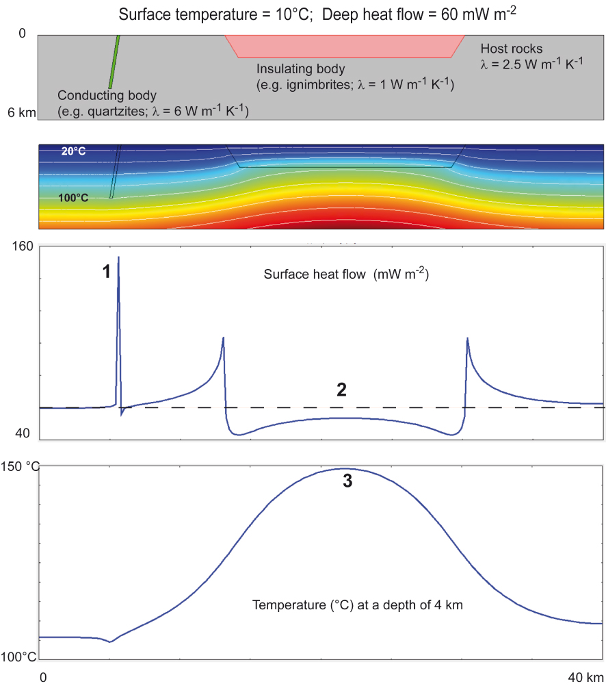
Case of heat refraction due to lithological contrasts. From top to bottom: geometries, boundary conditions, and physical properties; temperature field with isotherms in white contours separated by 20 °C; surface heat flow; horizontal temperature profile at a depth of 4 km. A conductive and narrow body (in green on the top image) does not disturb the isotherms (white contours) but results in an elevated surface heat flow (label 1). On the opposite, the large and insulating body (in pink on the top image) results in an important uplift of the isotherms, but a small heat flow anomaly (label 2). However, a temperature of almost 150 °C is present at a depth of 4 km (label 3). Masquer
Case of heat refraction due to lithological contrasts. From top to bottom: geometries, boundary conditions, and physical properties; temperature field with isotherms in white contours separated by 20 °C; surface heat flow; horizontal temperature profile at a depth of 4 km. A ... Lire la suite
On the contrary, when large thermally insulating bodies are present (e.g., a porous sedimentary layer or a thick sequence of ignimbrites, pink horizontal body on top of Figure 1), the isotherms are uplifted and a positive thermal anomaly develops (Figure 1, label 3). However, the product of the low thermal conductivity by an elevated temperature gradient may result in a normal surface heat flow (Figure 1, label 2). In this case, the underlying thermal anomaly (150 °C at a depth of 4 km, label 3) cannot be inferred by looking at surface heat flow data only.
Furthermore, thermal conductivity is also influenced by various factors such as temperature, the dominant mineral phase, porosity and saturating fluid, and anisotropy [Clauser and Huenges 1995]. All these factors may significantly affect the bulk thermal conductivity of the rocks. For example, anisotropy of thermal conductivity should be considered in sedimentary layers, especially in shales and clay-rich rocks [e.g., Davis et al. 2007].
One consequence of these simple heat refraction effects is that geothermal exploration may be underdeveloped if thermal features are considered through heat flow data only. To estimate correctly the underground temperatures, any analysis of heat flow data should be accompanied by an analysis of thermal conductivity data.
2.3. Thermal features at Soultz-sous-Forêts (upper Rhine graben, France)
The geothermal site of Soultz-sous-Forêts is a striking example of what is addressed in this study. Over the 20 km surrounding the area, high surface heat flow values range between 121 and 183 mW⋅m−2 [Lucazeau 2019], probably due to a large-scale anomalously high mantle heat flow, associated with the formation of the European Cenozoic Rift System [Dèzes et al. 2004]. However, this high surface heat flow is not accompanied by hot springs or other surface manifestations of underlying geothermal activity.
The presence of an anomalous surface temperature gradient in the area was established at the beginning of the XXth century when tens of boreholes were drilled in the Pechelbronn oil field, a few kilometers east of Soultz-sous-Forêts. With the available bottom-hole temperature measurements, Haas and Hoffmann [1929] established a temperature map at a depth of 400 m and discovered the thermal anomaly of Soultz-sous-Forêts (around 55 °C at a depth of 400 m). Before deep (up to five kilometers) boreholes were drilled at Soultz-sous-Forêts, the available subsurface temperature gradient measured at depths of a few hundred meters was exceptionally high (110 °C⋅km−1). Thus, the existence of a high-temperature geothermal reservoir at a shallow depth (estimated around 170 °C at a depth of 1.5 km, black star in Figure 2a, or between 140 and 180 °C at a depth of 1900 m, black rectangle in Figure 2a) was then suggested [Gerard and Kappelmeyer 1987]. In the late 80’s and in the 90’s, when the first shallow boreholes at Soultz were deepened to greater depths, it turned out that a temperature of only 140 °C was reached at a depth of 2 km, and only 200 °C at a depth of 5 km [Genter et al. 2010; Figure 2a]. The regularly decreasing temperature gradient from 1 km to 3.5 km depth represents the vertical extent of a nearly isothermal reservoir, where hydrothermal convection dominates and homogenizes temperatures [Clauser and Villinger 1990; Guillou-Frottier et al. 2013]. Similar temperature–depth profiles (an elevated surface temperature gradient and a nearly isothermal reservoir over several kilometers) were indeed measured in many other high-temperature geothermal systems (see examples of such temperature profiles in Figure 2b).
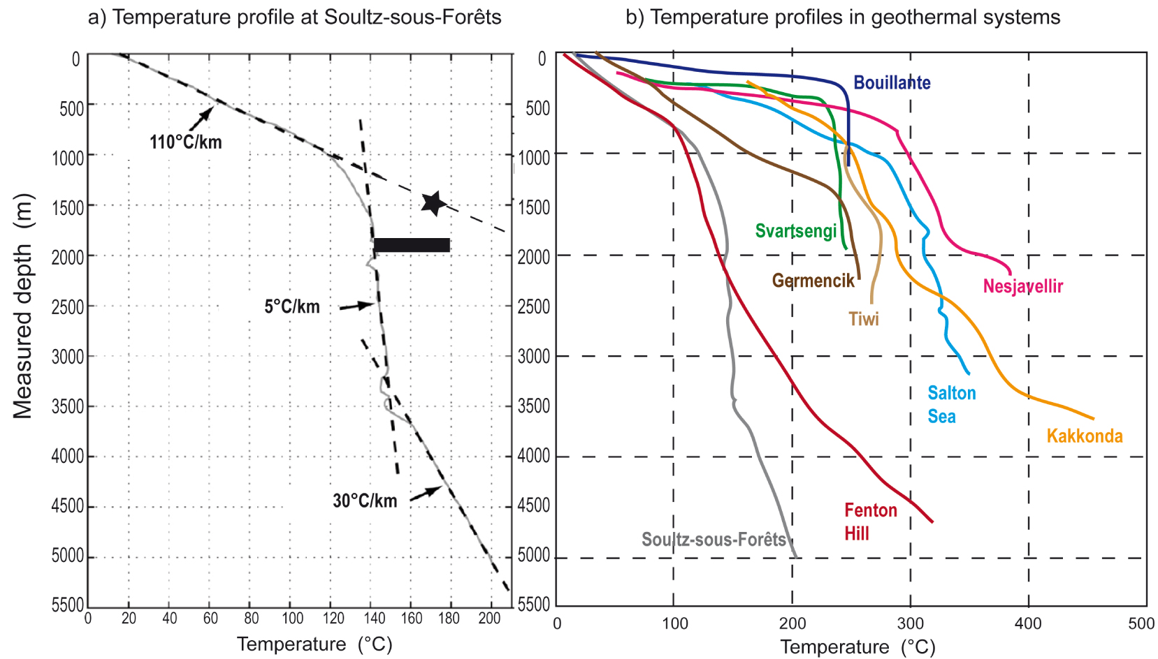
Temperature profiles in geothermal systems: (a) measured temperature profile (grey) in the GPK2 borehole at Soults-sous-Forêts (Alsace) and modifications of the temperature gradient (dashed lines), after Genter et al. [2010]. The black star and the black rectangle indicate the predictions in 1987 (see text). (b) General shape of temperature profiles in different geothermal systems: Fenton Hill [Harrison et al. 1986], Svartsengi and Nesjavellir [Steingrímsson 2013], Germencik Inanc Tureyen et al. [2014], Bouillante [Guillou-Frottier 2003], Tiwi [Moore et al. 2000], Salton Sea [Sass et al. 1986], Kakkonda [Doi et al. 1998]. Masquer
Temperature profiles in geothermal systems: (a) measured temperature profile (grey) in the GPK2 borehole at Soults-sous-Forêts (Alsace) and modifications of the temperature gradient (dashed lines), after Genter et al. [2010]. The black star and the black rectangle indicate the predictions in ... Lire la suite
With the example of Soultz-sous-Forêts in mind, where no hot springs or fumaroles are visible, one may postulate that the discovery of new high-temperature geothermal systems is still plausible, as soon as hydrothermal convection can occur in the shallow crust. The occurrence of hydrothermal convection requires that the host rock must be sufficiently permeable. Since the density of hydrothermal fluids is temperature-dependent, whatever the fluid composition, hot and light fluid at a depth of several kilometers would naturally rise to shallow levels, where less permeable rocks will enclose the geothermal reservoir.
Beside the occurrence of buoyancy-driven convection [or “free” convection, as detailed in Alt-Epping et al. 2021], non-Rayleigh convection and topography-driven (“forced”) convection may play a significant role in fluid flow and thermal regimes. In this study, although we put forward the role of damage zone geometry (Section 4.3) on the occurrence of buoyancy-driven convection (see Section 5.2), the other driving forces are also considered (topography-driven and poro-elasticity-driven forces).
3. Large-scale (10–1000 km) thermal anomalies: geodynamical control
3.1. Large-scale heat flow anomalies
Although lithological contrasts may result in small-scale discontinuous heat flow variations (Figure 1), long wavelength heat flow anomalies can be evidenced by interpolation maps such as the one published by Artemieva and Mooney [2001] (Figure 3). Anomalous heat flow values [higher than the average continental heat flow of 67 mW⋅m−2, Lucazeau 2019] can be delineated over several hundreds of kilometers. In southeast Australia (Figure 3a), a ∼250 km large zone shows high heat flow values (92 ± 10 mW⋅m−2), which are interpreted as resulting from high heat production of basement rocks [an average value of 6 μW⋅m−3 is obtained, instead of less than 3 μW⋅m−3 outside the area; Neumann et al. 2000].
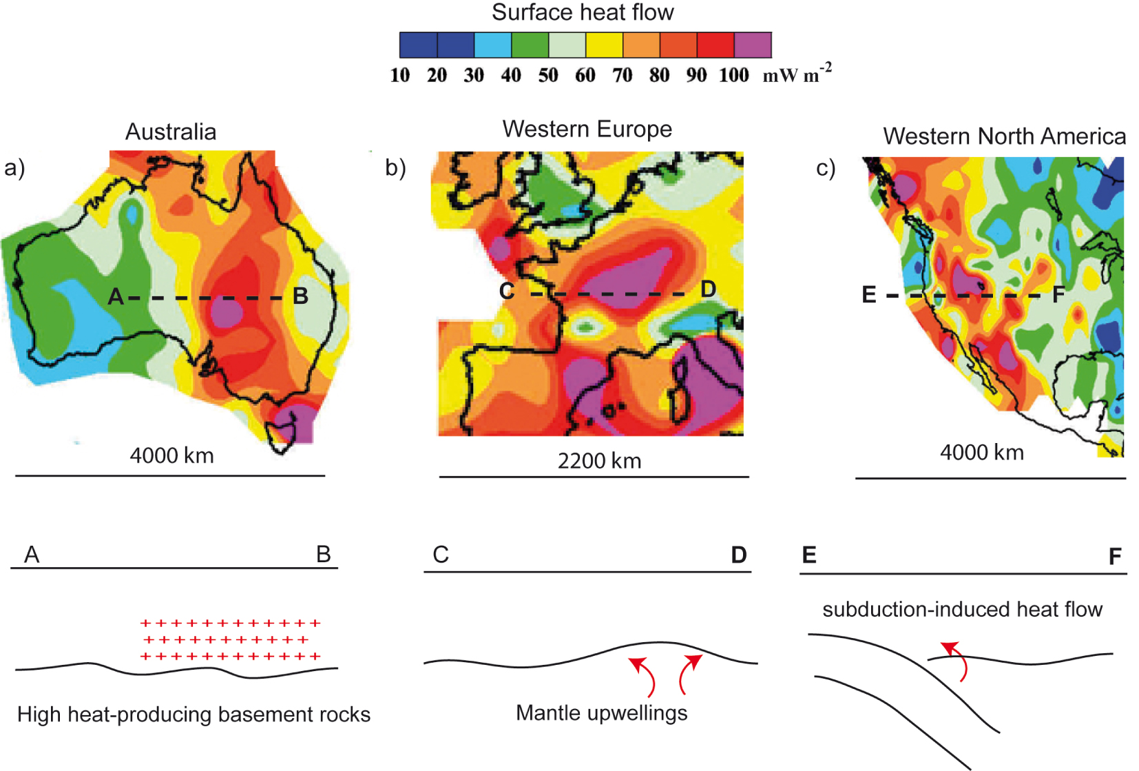
Three examples of interpolated maps of surface heat flow data (top), from Artemieva and Mooney [2001], and synthetic west-east cross-sections of geodynamic contexts (bottom). Long wavelength heat flow anomalies (from red to purple) are visible in southeast Australia (a), from the French Massif Central to the Rhine graben (b), and in western North America (c).
In the French Massif Central (Figure 3b), a broad zone of heat flow values exceeding 100 mW⋅m−2 can be delineated over a distance of ∼300 km [Lucazeau and Vasseur 1989]. Lucazeau et al. [1984] showed that crustal heat production alone cannot explain this long wavelength anomaly. They suggest that an additional mantle heat flow component, reaching 25–30 mW⋅m−2 (resulting in a maximum mantle heat flow around 60 mW⋅m−2) and associated with the recent Cenozoic activity, corresponds to the signature of a mantle diapir. According to recent thermo-mechanical models of plume–lithosphere interactions, small-scale mantle upwellings (or “baby-plumes”) might have played a significant role in continental rifting [Koptev et al. 2021].
The third example (Figure 3c) illustrates the long wavelength heat flow anomaly along the western coast of North America, below which the Farallon oceanic plate had subducted. Erkan and Blackwell [2008] detailed the different subduction-related geodynamical events that could explain the large-scale positive and negative heat flow anomalies. In particular, the geothermal systems of the Basin and Range Province, Nevada, would be associated with subduction-induced extensional tectonics and with surface heat flow higher than 80 mW⋅m−2 [Wisian and Blackwell 2004]. Slab tears and their thermal consequences might also have played a role in establishing this large-scale heat flow anomaly, promoting the melting of the ascending asthenosphere, particularly in the northeast portion of Baja California region [Ferrari et al. 2018]. At smaller scales, the high surface heat flow values in western Anatolia, Turkey, could be related to underlying subduction-related mantle flow (slab rollback and slab tear processes), inducing high mantle heat flow [e.g., Roche et al. 2018, 2019]. Similar processes may be at the origin of the extensional tectonics in Tuscany, Italy, where the Larderello-Travale geothermal field is characterized by an high regional surface heat flow exceeding 100 mW⋅m−2 over more than 100 km [Bonini et al. 2014].
3.2. Effect of mantle heat flow on crustal temperatures
The previous examples suggest that deep thermal anomalies that occurred in the past have diffused towards the surface, leaving a thermal imprint that can be deciphered today. Figures 4a and b illustrate the effect of mantle heat flow (Qm) on steady-state crustal temperatures for a three-layer crust, where heat production rates are twice as large as the ones described for an averaged crustal composition. A 35 km thick crust is made of a 13 km thick upper crust (thermal conductivity of 3.0 W⋅m−1⋅K−1, heat production of 3.2 μW⋅m−3), an intermediate 11 km thick crust (2.5 W⋅m−1⋅K−1 and 1.5 μW⋅m−3) and a 10 km thick lower crust (2.0 W⋅m−1⋅K−1 and 0.4 μW⋅m−3). For this model, the crustal component reaches 62.1 mW⋅m−2. A mantle heat flow of 20 mW⋅m−2, leading to a surface heat flow (Qs) of 82.1 mW⋅m−2, is not sufficient to get 150 °C in the first 6 km of the crust. However, a Qm value of 50 mW⋅m−2 (Qs = 112.1 mW⋅m−2) allows such high temperatures, but only below a depth of 4 km. Figure 4c illustrates the transient effect of a thermal pulse coming from the mantle. Considering the steady-state temperature profile of Figure 4a with a mantle heat flow value of 20 mW⋅m−2, an instantaneous thermal pulse of 30 mW⋅m−2 (providing a mantle heat flow of 50 mW⋅m−2) is applied during 10 Myrs. Mantle heat flow is then reduced instantaneously to its initial value of 20 mW⋅m−2. It results that the induced temperature change at a depth of 5 km does not exceed 24 °C. For a thermal pulse of 50 mW⋅m−2, temperatures exceeding 150 °C are found below a depth of 4100 m.
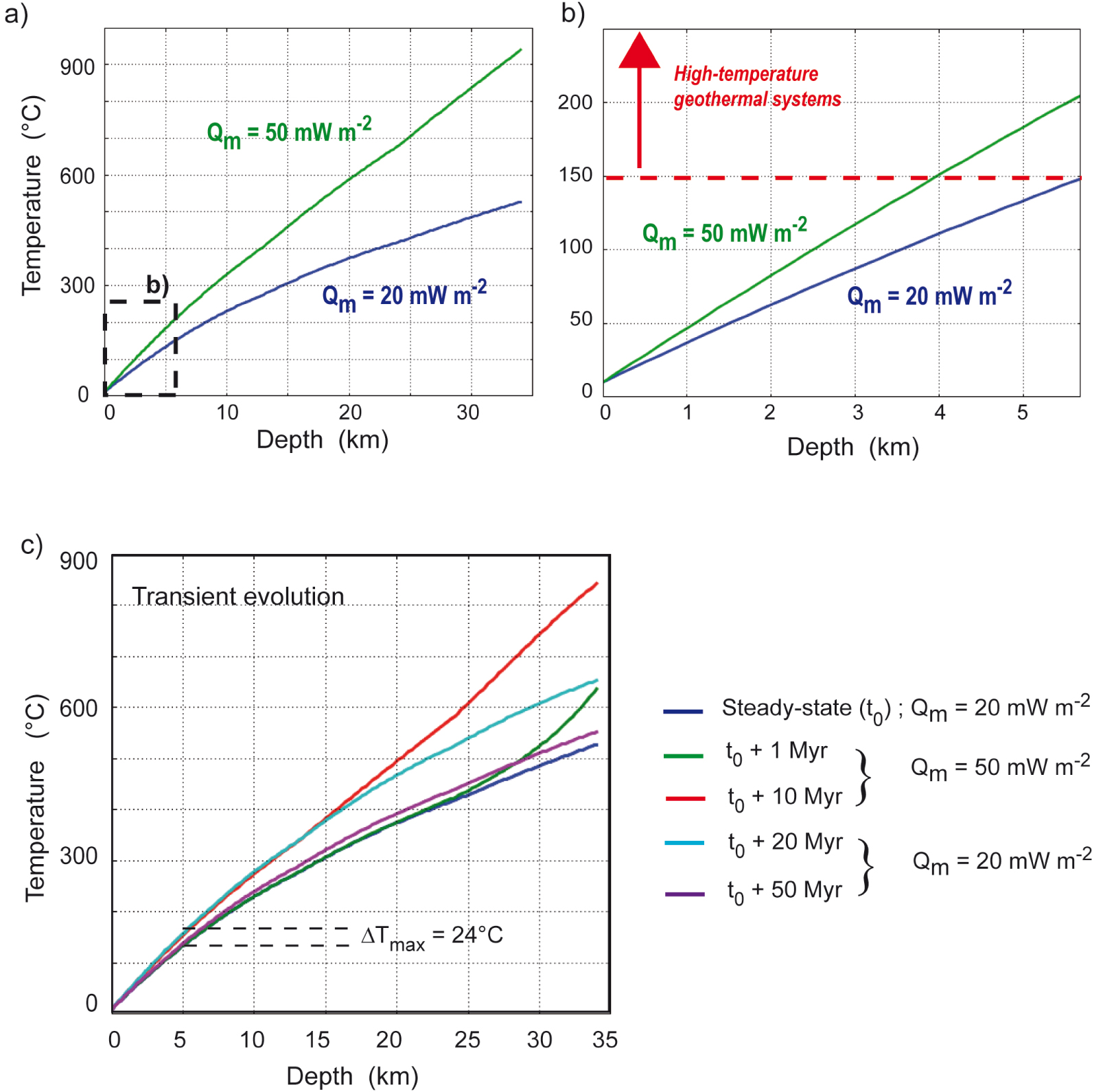
Effect of mantle heat flow on temperature–depth profiles for a three-layer crust enriched in radioactive elements (see Section 3.2). The crustal geotherms on the left (a) are zoomed at shallow depth in (b), where the red arrow indicates the temperature domain for high-temperature geothermal systems; (c) transient effect of an instantaneous increase of Qm (from 20 to 50 mW⋅m−2 during 10 Myrs).
In summary, whatever the chosen crustal models, in the absence of shallow magmatic intrusions, and for reasonable values of heat production rates (from 0.5 μW⋅m−3 in the lower crust to 4.0 μW⋅m−3 in the upper crust), temperatures above 150 °C are difficult to be reached at shallow depths (1–4 km). If heat transfer occurs only by conduction, then abnormally high heat production rates are required, as for some Australian granites. Otherwise, high temperatures (>150 °C) at shallow depths can only be reached if fluid circulation is taken into account.
4. Small-scale (0.1–10 km) thermal anomalies: structural control
This section is dedicated to abnormally permeable zones of the crust, particularly fault zones within which fluid circulation induces thermal anomalies at shallow depths (Section 5). Here, we first focus on crustal permeability and transient effects on permeability as detailed in Taillefer [2017], and then on fault zone architecture and damage zone properties.
4.1. Crustal permeability
Permeability is a key parameter that controls the occurrence of fluid flow (whether driven by topography or buoyancy) and thus the location and the amplitude of thermal anomalies [e.g., Taillefer et al. 2018; Guillou-Frottier et al. 2020; Alt-Epping et al. 2021]. Crustal permeability is considered to be strongly depth-dependent [Anderson et al. 1985; Ingebritsen and Manning 1999; Shmonov et al. 2003; Saar and Manga 2004; Stober and Bucher 2007; Earnest and Boutt 2014; Ranjram et al. 2015], and recent studies showed that the permeability at depth is the main parameter that controls the longevity of a geothermal system [e.g. Ingebritsen and Gleeson 2017]. Exponential first-order relationships were established between permeability and depth [Anderson et al. 1985; Shmonov et al. 2003; Saar and Manga 2004], and the few hydraulic data on crystalline rocks [Stober and Bucher 2007] seem to confirm this dependence (red curve in Figure 5). However, based on large data sets, recent studies showed that permeability values in the shallow crust (<2.5 km) are mainly controlled by lithology [Neuzil 2019, Figure 5] and tectonic setting [Ranjram et al. 2015]. Unfortunately, permeability evolution in the targeted depth window for geothermal energy (1–4 km), is still not well constrained due to the lack of data [Stober and Bucher 2007; Ranjram et al. 2015].
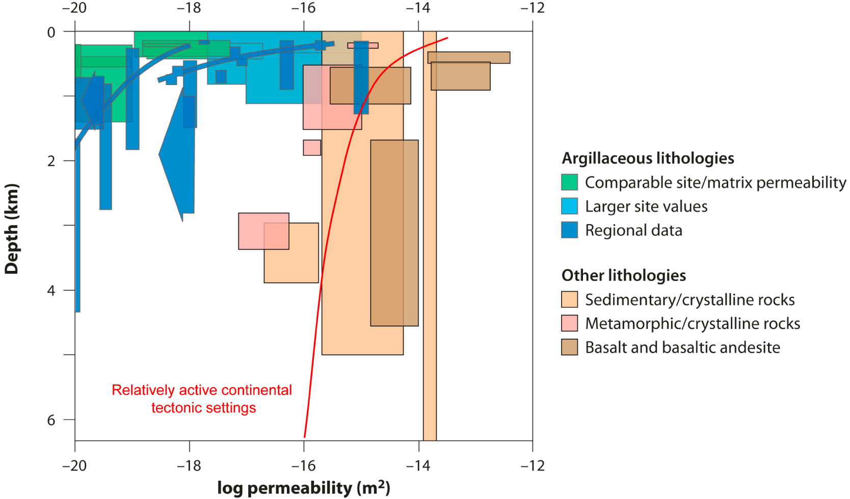
Range of permeability (m2) vs. depth (km) for different lithologies in the brittle continental crust [modified after Neuzil 2019]. Green and blue are site (10−2–102 km2) and regional (103–106 km2) clay and shale data, other colors are sedimentary/crystalline rocks and metamorphic/crystalline rocks [Townend and Zoback 2000], except brown for basalt and basaltic andesite [Saar and Manga 2004]. The red curve represents hydraulic data from Stober and Bucher [2007].
The high sub-surface permeability (Figure 5) is related to supergene alteration processes and the fractured decompression zone [Dewandel et al. 2006]. Interestingly, rocks affected by weathering can preserve these high permeability characteristics when subsequently buried [Lachassagne et al. 2011]. This is the case at Soultz-sous-Forêts, where the permeability of the altered and fissured horizon at the top of the granitic basement is preserved at depth [Genter et al. 2010].
Fractures can increase the permeability of protoliths by several orders of magnitude [Sonney and Vuataz 2009; Cox et al. 2015]. Because of their interconnection, the set of fractures is also called a “fracture network”, whose permeability is dependent on several factors such as the fracture morphology, the spatial organization of the fracture network (density and connectivity), the fillings, and the ongoing tectonic activity that keeps the fractures open [Crider 2015]. Fractures can be closed under confining pressure, or cementation, if they are not held open by tectonic stresses or fluid pressure [Laubach et al. 2004]. Larger stress magnitudes in tectonically active regions may produce, at depth, fracture apertures larger than expected [Earnest and Boutt 2014]. Fracturing associated with the fault zones will have a significant impact on creating or maintaining permeability, particularly at the depths targeted for deep geothermal energy (1–4 km).
4.2. Transient effects on permeability variations
The fractures, the fluid pressure, and the fluid composition play a key role in the permeability evolution of the geothermal system [Renard et al. 2000]. Numerous studies on hydrothermal systems show that the permeability varies in time as well as space [e.g., Cox et al. 2015]. It is therefore relevant to consider the concept of “dynamic permeability” [Ingebritsen and Gleeson 2017] and detail the transient effects that can impact a geothermal system. In particular, mineralization processes, or fault activity and consequent fluid flow may decrease or increase permeability, respectively, as detailed below.
The whole process of fracture sealing by mineralization plays an important role in the lifespan of a geothermal system, and can significantly reduce its permeability [Renard et al. 2000; Griffiths et al. 2016]. Rock/fluid interaction will be responsible for the nature of mineralization, and mineralization can completely block fluid circulation [Staněk and Géraud 2019]. Renard et al. [2000] show that at the scale of a fracture, pressure/solution mechanisms are faster (a few years) than fracture cementation (from a hundred years to several million years), allowing fluid circulation to be maintained over time. In fault zones that localize fluid circulation, the presence of phyllosilicates and clays is frequently reported [e.g., Nishimoto and Yoshida 2010], and can change the permeability properties [e.g., Yielding et al. 1997; Leclère et al. 2012].
Fault activity can increase permeability. Major tectonic setting changes can lead to migration or modification of the main parameters of the geothermal system: spring location, flow rates and temperatures [Husen et al. 2004; Ingebritsen and Manning 2010; Cox et al. 2015; Taillefer et al. 2021]. Faulds et al. [2010] showed that, in the Basin and Range (western USA), geothermal systems are more likely associated with active faults. However, the macro-seismicity is not a critical parameter for the preservation of a permeable fracture network, if a favorably oriented stress regime can maintain the permeability required for fluid flow [Barton et al. 1995; Townend and Zoback 2000]. In this case, geothermal systems reach a state of equilibrium allowing constant hydrothermal activity [Taillefer et al. 2018].
The fluid flow itself influences permeability with fluid overpressures in low-permeability or sealed zones [Sibson 1992]. When these overpressures are located along a fault, they can initiate slip on the fault and associated earthquakes [Cox 2016]. Such a fault-valve behavior [Sibson 1992] allows post-failure discharge of fluids. Importantly, in most cases, this leads to the upward migration of fluids along the fault. In addition, the activity of the fault related to these overpressures allows the re-opening of closed or sealed fractures, and the generation of new fractures [Schoenball et al. 2020].
Finally, climatic factors can also influence fluid flow in a geothermal system. Water from numerous geothermal systems has a meteoric origin [e.g., Grasby and Hutcheon 2001; Sonney and Vuataz 2009; Diamond et al. 2018], and therefore depends on climatic conditions. Fluid flow and temperature of the water can be correlated with rainfall [Ratouis et al. 2017]. It is important to note that rainfall correlation is not systematic for a long geothermal cell [Taillefer et al. 2018]. Recent studies by Alt-Epping et al. [2021, 2022] demonstrated that flow patterns can change during periods of glaciation. For example, non-Rayleigh convection during glacial periods would evolve towards topography-driven flow during interglacial periods. Glaciation can also have several implications: (1) the loading effect of glaciers causes local variations in stress [Neuzil 2012]; (2) the melting of ice and the associated infiltration of cold fluids leads to a cooling of the massif [Maréchal et al. 1999]; (3) the thickness of ice on the relief can reduce the infiltration of meteoric water [Volpi et al. 2017].
4.3. Fault zone architecture and damage zone thickness
The fault zones constitute one of the most permeable zones in the Earth’s crust (see Sections 4.1 and 4.2). It is therefore relevant to detail the main characteristics and the fracturation volume associated with these structural objects. Two main zones are distinguished inside a deformed and altered rock volume in a fault zone: (i) one, or several Core Zone(s) (CZ) characterized by the presence of fault rocks frequently associated with clay or thin matrix (<0.1 mm) and well-developed cementation. These zones are mostly recognized as a barrier for fluid circulation when the fault is not active [e.g. Sibson 2000; Fossen 2016]. (ii) two, or several Damage Zone(s) (DZ), characterized by an increase in fracture density compared to the protolith [e.g. Sibson 2000; Faulkner et al. 2003]. The damage due to the fault activity increases the permeability of the protolith by several orders of magnitude, thus allowing fluid circulation [Mitchell and Faulkner 2012]. The damage zone is composed of an inner part, highly fractured, commonly associated with intense fluid circulation and an outer part, less fractured, but still more permeable than the protolith [e.g., Choi et al. 2016].
The degree of maturity of the fault exerts a strong control on the thickness of the DZ that localizes the maximum permeability. Figure 6 shows that the thickness of the DZ is correlated to the fault displacement, a proportional relationship exists for displacement until ∼150 m, regardless of the kinematic of the fault and the nature of the protolith [Bense et al. 2013; Mayolle et al. 2021]. Above 150 m, DZ thickness is limited to a few hundred meters [e.g., Mitchell and Faulkner 2009; Bense et al. 2013; Mayolle et al. 2019]. Characterization of the DZ thickness for faults with displacement above hundred meters shows more uncertainty due to the presence of secondary faults and the difficulty to find a continuous outcrop for fracture quantification [Choi et al. 2016]. Several models are proposed for the bending of the DZ thickness observed in Figure 6: the thickness of the brittle crust [Ampuero and Mao 2017], segmentation of the fault [Schlische et al. 1996]; accumulation of displacement and fault damage thickness by incorporating damages from the former fault segments [Mayolle et al. 2019, 2021, and references therein]. Along pluri-kilometric faults, the geometry of the fault itself has a strong control on the permeability. Indeed, fault relays, fault terminations and fault intersections are more favorable zones to channel fluid circulation due to an increase in fracture density [Curewitz and Karson 1997; Faulds and Hinz 2015].
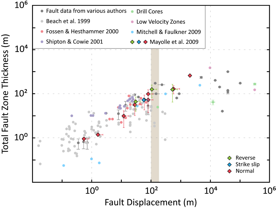
Total fault zone thickness as a function of displacement, modified from Mayolle et al. [2019]. The damage zone thickness is defined as the total adjacent damaged rock volume on both sides of the fault. The bending of the linear scaling law trend is highlighted in light brown.
5. Fluid circulation in fault geothermal reservoirs
Fluid flow in a permeable medium can be due to different driving forces [Alt-Epping et al. 2021]. In our study, the permeable medium consists of a finite width fault zone. Thus, the classical Rayleigh number expression does not apply (see Section 5.2). Although we mainly focus our study on buoyancy-driven convection, topography-driven and poro-elasticity-driven forces will be also investigated (Sections 5.3 and 5.4). The effects of fault thickness, the impact of tectonic regimes or the role of the poro-elasticity force are discussed but not compared to each other. This section is thus dedicated to illustrate independently different causes leading to the establishment of shallow thermal anomalies.
5.1. Fluid flow in fault zones and related thermal anomalies
Apart from geological evidence of fluid circulation within fault zones (see Section 4), theoretical and numerical studies brought quantitative aspects related to the required conditions for thermal convection to occur [Forster and Smith 1989; Malkovsky and Magri 2016]. When buoyancy-driven flow occurs within a fault zone, temperature anomalies develop and may result in large volumes of high (>150 °C) temperatures at shallow depths (1–4 km). For example, Wanner et al. [2019] suggested that large ellipsoidal thermal plumes are generated by fault-hosted orogenic geothermal systems, such as the Grimsel Pass case, Swiss Alps, where hot upwellings would provide hundreds of PJ (1015 J) of anomalous heat per km depth. Guillou-Frottier et al. [2020] illustrated similar convective patterns where temperature anomalies may exceed 70 °C at a depth of 500 m. These studies demonstrate that temporal and spatial variations of permeability play a key role in the morphology and amplitude of temperature anomalies. They also show that temperature anomalies are larger and higher for vertical fault zones [see also Duwiquet et al. 2019] and for wide damage zones. Because damage zone thickness may exceed several hundreds of meters, it is worth studying through simple theoretical considerations how fault zone thickness influences thermal convection features.
5.2. Role of fault zone thickness
Malkovsky and Magri [2016] studied the conditions for which thermal convection occurs within a fault zone of thickness 2𝛿 and height H, embedded into impermeable rocks. They extended the constant viscosity case developed by Malkovsky and Pek [1997] by considering a temperature-dependence of the fluid viscosity (as for the case of hydrothermal fluids), characterized by a dimensionless parameter, 𝛾. Their linear stability analysis provides a new expression for the critical Rayleigh number Racrit, where the fault aspect ratio 𝛥 =𝛿 ∕H appears:
| (2) |
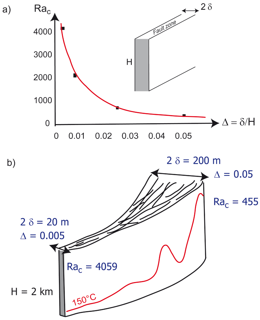
(a) Role of the fault thickness (2𝛿) (or half-thickness over height ratio, 𝛥) on the critical Rayleigh number, after the theoretical law of Malkovsky and Magri [2016]; (b) sketch of a fault zone whose thickness increases from 20 m to 200 m: the critical Rayleigh number decreases by a factor 9, and isotherms can be strongly distorted within the wide part.
When the Rayleigh number expression is considered [see Equation (12a) in Malkovsky and Magri 2016], the critical permeability above which convection occurs can be estimated for different 𝛥 ratios. The fault zone height is here fixed at 5 km, and a temperature difference of 200 °C is assumed, while other physical properties are well-known. For a fault thickness of 100 m (𝛿 = 50 m; 𝛥 = 0.01), the critical Rayleigh number equals 2050 (Figure 7a) and the critical permeability above which thermal convection occurs equals 2.6 × 10⁻¹⁴ m2. For a fault thickness of 500 and 1000 m, the critical permeability decreases to 5.9 × 10⁻¹⁵ m2, and to 1.4 × 10⁻¹⁵ m2, respectively.
However, these estimates depend on several hypotheses, such as the chosen expression of the Rayleigh number [see Equations (12a) and (12c) in Malkovsky and Magri 2016]. Another way to understand qualitatively the role of fault thickness on the temperature field is to run simple 2D numerical experiments where realistic physical parameters are chosen and where the thickness of the damage zone varies. This 2D simplification is valid as soon as fault length can be considered pluri-kilometric. The numerical procedure and set-up are detailed in the Appendix A. Thermal convection occurs within the fault damage zone, and the maximum temperature at different depths is recorded. Figure 8a illustrates this maximum temperature at a depth of 3 km in a fault zone permeability–fault zone width diagram. For example, for a fault width of 800 m where permeability equals 5 × 10⁻¹⁵ m2, 120 °C can be reached at a depth of 3 km. To get 150 °C for the same fault width, permeability must be larger than 3 × 10⁻¹⁴ m2. Figure 8b illustrates the depths for which 100, 120 and 140 °C are observed, for four different fault widths. For large fault thicknesses, temperatures above 100 °C are observed at depths lower than 2 km. On the right of light orange areas (conductive regimes), maximum temperatures are controlled by the convective regimes, where downwellings or upwellings can decrease or increase the maximum recoded temperature.
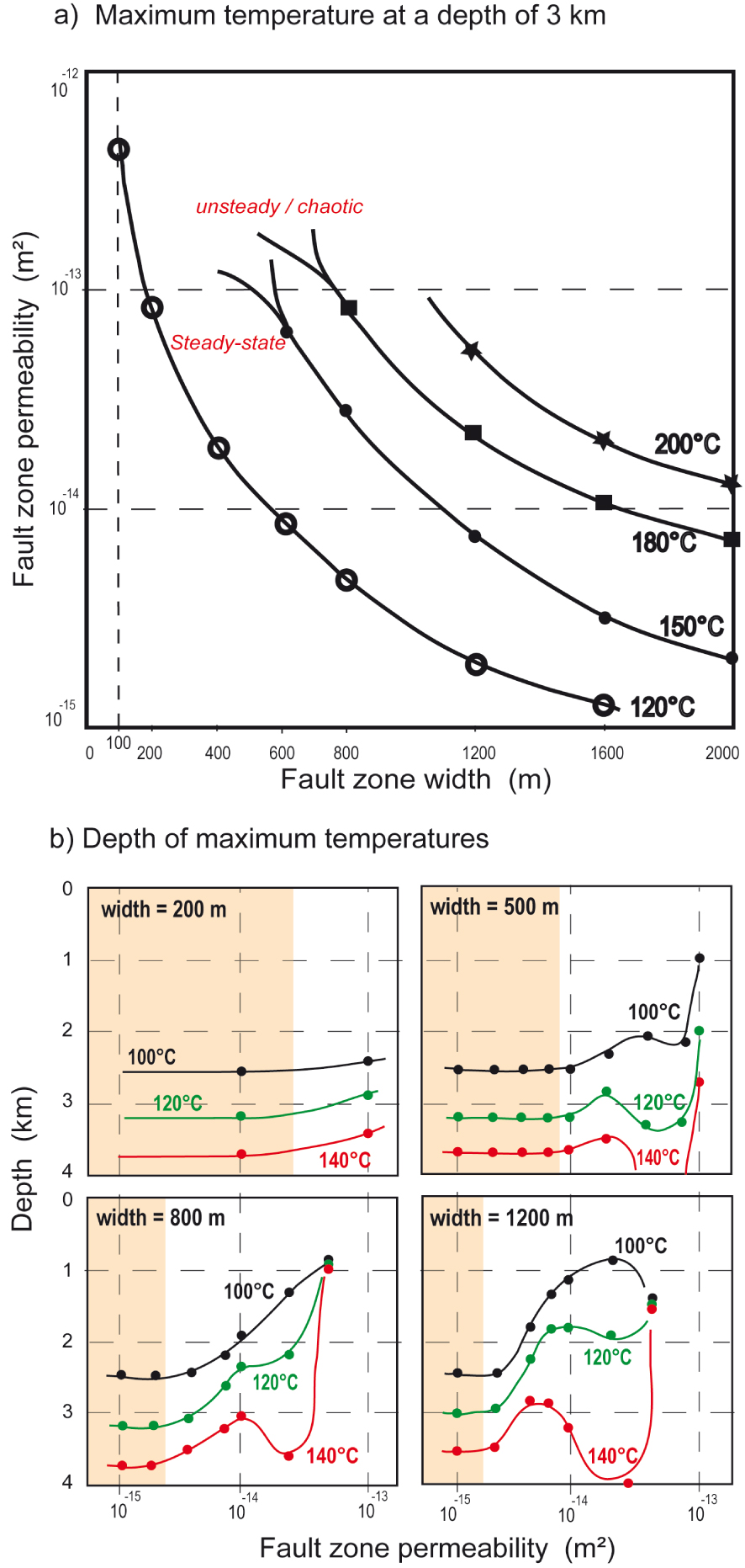
Results from 2D numerical models of thermal convection within a fault-damage zone (see details in the text and Appendix A). (a) Maximum temperature observed at a depth of 3 km. For a 600 m wide damage zone, the temperature reaches 150 °C for a permeability of 6 × 10⁻¹⁴ m2. If the fault-damage zone is twice as wide (1200 m), 150 °C is reached for a permeability of 7.5 × 10⁻¹⁵ m2. Curves for 120 °C, 180 °C, and 200 °C are also shown. (b) Depths of maximum temperatures observed (100, 120 and 140 °C) for different fault widths as a function of fault zone permeability. Areas in light orange correspond to conductive regimes. Masquer
Results from 2D numerical models of thermal convection within a fault-damage zone (see details in the text and Appendix A). (a) Maximum temperature observed at a depth of 3 km. For a 600 m wide damage zone, the temperature reaches 150 °C for a ... Lire la suite
5.3. Impact of tectonic regimes
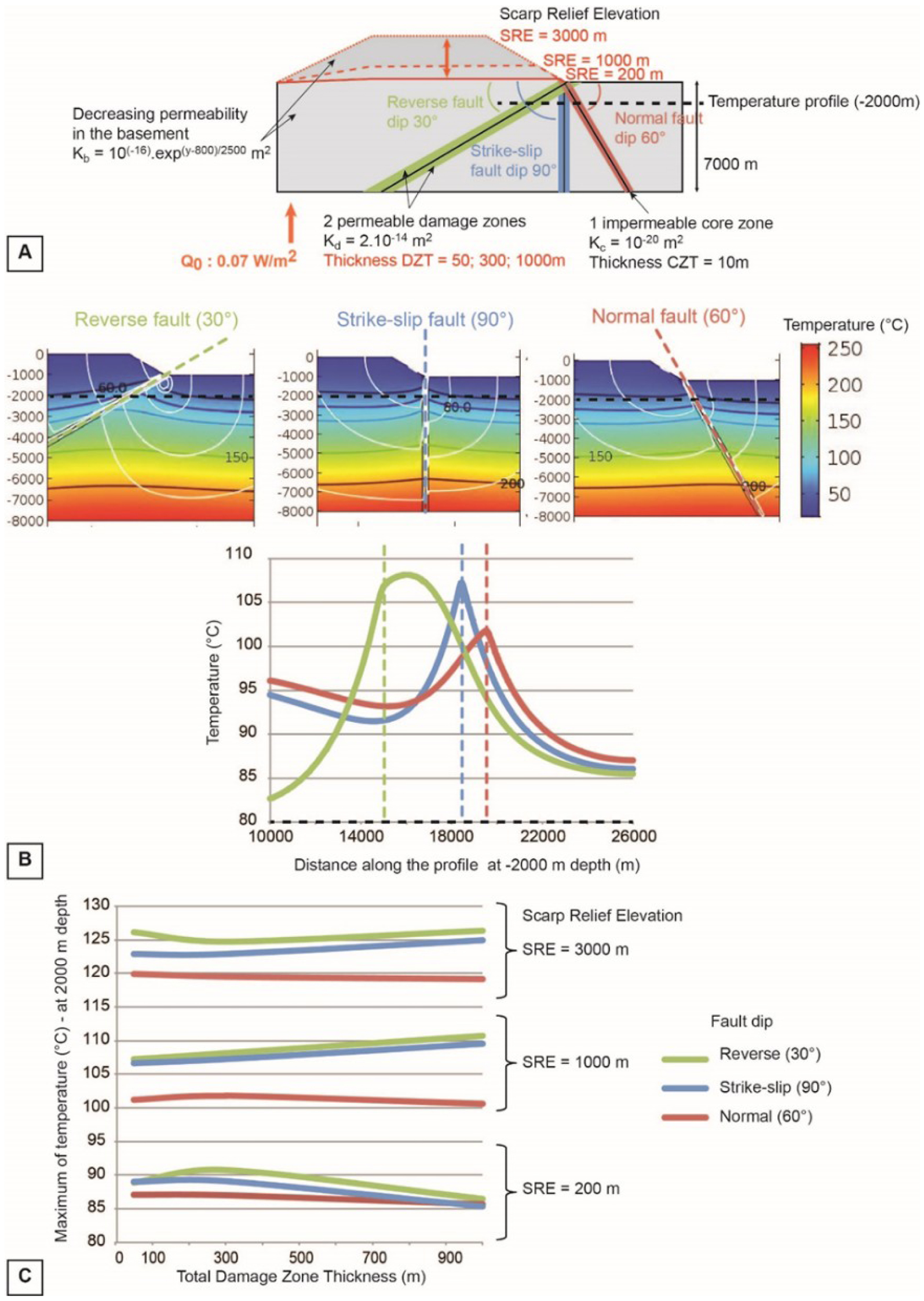
The three basic tectonic regimes, that is, extensional (normal), compressional (reverse), and strike-slip, result from different stress fields and express themselves in the field by typical geometric and geomorphologic features (e.g., fault dip, form of the scarp relief). Some of these differences are here tested in a 2D parametric study considering a fault zone and its related topography in only one of the fault compartments (Figure 9a). Mechanical stresses are not explicitly taken into account in these models, where only thermal and hydraulic processes are coupled, but their effects on fault geometry and geomorphology are reproduced.
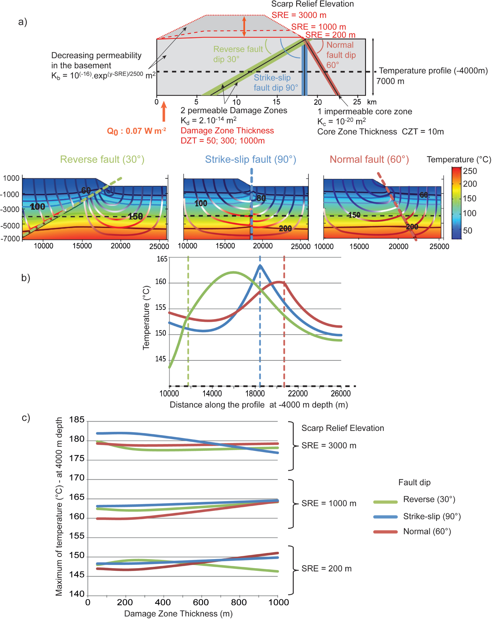
Parametric study on the geometric features of a scarp relief related to a fault offset. Colors associated with typical fault dips (green = reverse 30°, blue = strike-slip 90°, normal = 60°) are common to the three figures. (a) Sketch of the numerical model, the tested parameters are in red. (b) Influence of the fault dip on the temperature distribution (color chart), along a profile at a depth of 4000 m below the flat right compartment (dashed black line). Thick and thin lines on the sketches correspond to the isotherms and flow lines (colored according to the temperature), respectively. Dashed colored lines correspond to the position of the core zone at the surface. (c) Comparison of the maximum temperatures reached at a depth of 4000 m for the three tested parameters. Masquer
Parametric study on the geometric features of a scarp relief related to a fault offset. Colors associated with typical fault dips (green = reverse 30°, blue = strike-slip 90°, normal = 60°) are common to the three ... Lire la suite
5.3.1. Numerical model
The numerical model is a 2D-block consisting of two compartments of the basement with a depth-decreasing homogeneous permeability. A fault zone composed of one 10 m-thick core zone with a constant permeability Kc, surrounded by two damage zones with a constant permeability Kd, separates the two compartments. The choice of a constant permeability Kd may be questionable since it may depend on the tectonic regime. However, based on the Scibek database [2020], we estimate an average permeability of fault zones around 10−14 m2, whatever the tectonic regime. We thus fixed this value to allow fluid circulation within damage zones for all experiments. The thickness of the total fault damage zone (DZT, two half damage zones) is tested for the values DZT = 50, 300, and 1000 m. The fault dip is tested through three typical dip values according to the main tectonic regimes: reverse (30°), strike-sip (90°), and normal (60°). The left basement compartment (i.e., the hanging wall of the reverse fault or the footwall of the normal fault) represents a scarp relief associated with the fault offset which elevation (Scarp Relief Elevation, SRE) is tested for the values SRE = 200, 1000, and 3000 m. The model is examined along a horizontal temperature profile at 4000 m below the surface without topography (i.e. the right compartment). A mixed thermal boundary condition is applied to the topographic surface. This mixed thermal condition relates the surface heat flow with surface temperature through a heat transfer coefficient [see details in Taillefer et al. 2018, and in the Appendix A]. This allows variations in surface temperatures, as illustrated by, e.g., the presence of hot springs [see also Magri et al. 2015]. The variables and parameters used in the models are available in the Appendix A.
5.3.2. Numerical results
5.3.2.1. Influence of the fault dip
The numerical results of Figure 9b represent the temperature, the main isotherms, and flow lines colored according to the fluid temperature inside the model for the three fault dips (FD) configurations. For greater readability, only the intermediate combination is presented in Figure 9b, i.e. SRE = 1000 m, DZT = 300 m, but all the parametric combinations were tested, and show similar patterns. The flow lines in Figure 9b show that cold fluids infiltrate at the model surface and then go down to depths of several kilometers under the effect of the pressure gradient. They warm during their descent under the effect of the geothermal gradient, and reach a temperature of 150 °C around a depth of 4000 m. These warm fluids are caught by the permeable damage zones where they can easily circulate and reach the surface. In any fault dip configuration, both the sketches and the temperature profiles at a depth of 4000 m show that the deformed isotherms at the fault vicinity create a positive thermal anomaly (Figure 9b). However, the amplitude and the form of this anomaly depend on the fault dip. The thermal anomaly associated with the reverse fault (FD = 30°) has the widest lateral amplitude and is off-center with respect to the core zone. Conversely, the strike-slip (FD = 90°) and the normal (FD = 60°) fault anomalies are centered on the fault core zones. The temperature anomaly related to the normal fault is asymmetric, with the temperature in the left (relief) compartment being more elevated than in the right (flat) compartment. The fault dip, i.e., the tectonic regime, could then strongly influence the temperature distribution at the fault zone vicinity.
5.3.2.2. Relative importance of the tested parameters on the maximum temperature
The maximum temperature reached along the horizontal temperature profile at a depth of 4000 m gives an estimate of the relative importance of the three tested geometrical parameters: the total damage zone thickness DZT, the scarp relief elevation SRE, and the fault dip FD (Figure 9c). The greatest influence on the maximum temperatures is related to the scarp relief elevation (with a maximum difference of 34 °C between SRE = 200 m and SRE = 3000 m): the higher the scarp elevation relief, the higher the temperature. Fault dip and damage zone thickness have a similar influence on the maximum temperature, with a maximum difference of 5 °C between normal and reverse fault (SRE = 200 m, DZT = 1000 m), and between a damage zone of 50 and 1000 m (SRE = 3000 m, strike-slipe fault), respectively. It seems that there are no clear rules about which fault dip or damage zone thickness is more adapted for reaching the highest temperatures at a depth of 4000 m. However, additional results (see Appendix A) show that at shallow depths (2000 m), fault dip has a stronger influence on the maximum temperatures (8 °C of difference), with reverse faults recording the maximum temperatures for all the parameter combinations. At these shallower depths, the damage zone thickness has a poor influence on the maximum temperature. Nevertheless, the impacts of the fault dip and damage zone thickness on the maximum temperature are weak compared to those due to the topography.
5.4. Role of the poroelasticity-driven force
Tectonic deformation influences fluid flow in different geological contexts [Bethke 1985; Rowland and Sibson 2004; Eldursi et al. 2021]. Within a basement fault zone, such as the one described above (i.e., an anomalously permeable zone), a single stress (SHmax) impacts the general convective dynamics and affects the thermal field [Duwiquet et al. 2021]. The distribution of positive and negative temperature anomalies in these permeable areas depends, among others, on tectonic regimes, whose poroelasticity-driven force has been identified [Duwiquet et al. 2022]. These effects were highlighted both by quantifying a very small permeability variation (less than 1%), but also by recording fluid pressure variations related to the tectonic regimes implemented.
Based on poroelasticity assumptions, we propose to investigate how the poroelasticity-driven force, caused by tectonic regimes, can have an impact on the fluid flow for a 0.3 km fault thickness (here the fault core is not taken into acount). This fault thickness is typical of natural fractured systems such as the Têt fault [Taillefer et al. 2018; Milesi et al. 2020] or the Seferihisar-Balçova fault-hosted geothermal system [Magri et al. 2012]. Considering a simplified 3D geometry and realistic physical properties [see Duwiquet et al. 2022, for details] the approach consists first in generating a numerical model without tectonic regime application (the benchmark experiment, Figure 10a). Thereafter, we applied two different tectonic regimes (Figure 10b, compression and extension, Figure 10c,d). A comparison between the benchmark experiment and the other simulations will be discussed, especially in terms of fluid pressure variation (Figure 10e). This comparison allows us to understand the different dynamic convective patterns obtained in the different numerical experiments, and how the poroelasticity-driven force could explain these differences. Note that this experiment is similar to the ones discussed in Duwiquet et al. [2022] except that fault thickness is here reduced to 0.3 km.
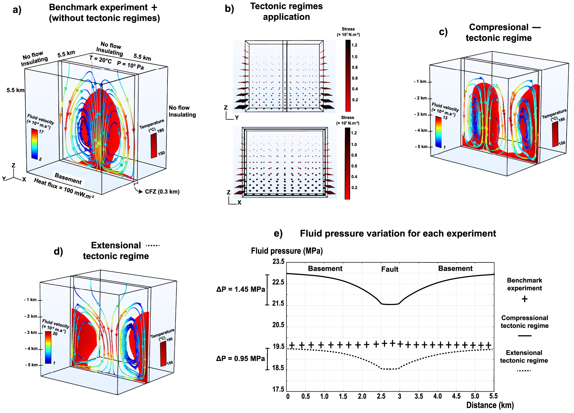
3D numerical model of hydrothermal convection within a 300 m wide fault zone embedded in impermeable rocks. A fixed temperature and a fixed pressure are imposed at the upper surface. The no-flow and insulating conditions apply to lateral boundaries. A fixed heat flux and a no-flow condition are imposed at the bottom boundary. Results correspond to a steady-state regime. (a) Boundary conditions and result for the experiment without applying tectonic stresses; (b) illustration of stress applications as boundary conditions for the compressional tectonic regime (with SHmax⩾Shmin⩾SV); (c,d): thermal (red color for temperature greater than 150 °C) and velocity fields (colored arrows along streamlines); (e) fluid pressure variations for each experiment. Masquer
3D numerical model of hydrothermal convection within a 300 m wide fault zone embedded in impermeable rocks. A fixed temperature and a fixed pressure are imposed at the upper surface. The no-flow and insulating conditions apply to lateral boundaries. A fixed ... Lire la suite
To investigate the influence of tectonic regimes on fluid flow, we used the Andersonian assumption, which is regularly used in geomechanical reservoir studies [Zoback et al. 2003]. The principal stresses are expressed with vertical (Sv), maximum horizontal (SHmax), and minimum horizontal (Shmin) components. Note that the relative stress magnitudes determine the modeled tectonic regime:
- Compressional (reverse/thrust faulting), with SHmax⩾Shmin⩾SV,
- Extensional (normal faulting) with SV⩾SHmax⩾Shmin.
As the model is aligned with the principal stresses, pure normal stresses are applied on the lateral boundaries. For the compressional tectonic regime, the fault is perpendicular to the SHmax stress while for the extensional tectonic regime, the fault is perpendicular to Shmin. In these models no shear is applied on the vertical boundaries. The depth-dependence of stresses is extracted from drilling measurements in the French Massif Central [Cornet and Burlet 1992] and is illustrated in Figure 10b. This implementation follows the method detailed in Duwiquet et al. [2022].
In the benchmark experiment (i.e. without tectonic regime application), the fluid shows an upward movement at the center of the fault zone (Figure 10a) and two downward movements on either side of the fault zone. Fluid flow velocities range from 2 to 17 × 10−9 m⋅s−1. The velocity is highest in the downward movements. The upward movements induce a rise of the isotherms. For example, the 150 °C isotherm target for geothermal energy is found at 1.2 km depth (Figure 10a), while in a pure conductive regime with no fluid flow, the 150 °C isotherm was observed at 5 km depth. Between the basement and the fault zone, no fluid pressure variation exists (Figure 10e). However, within the fault, there is a slight increase in fluid pressure, which is related to upward fluid movement. In light of these elements, buoyancy-driven forces alone act on fluid convection. After tectonic regime application (Figure 10b), the results are different (Figure 10c,d).
In the compressional tectonic regime (Figure 10c), the fluid pattern is characterized by two downward and two upward movements. The fluid velocities vary from 1 to 13 × 10−9 m⋅s−1, and the fastest velocities are found in the downward movements. The upward movements raise the 150 °C isotherm at a depth of 1.4 km. This convective dynamics differs from the benchmark experiment, (Figure 10a), as well as from the extensional tectonic regime. For the extensional tectonic regime (Figure 10d), the fluid patterns follow a downward and two upward movements. Fluid flow velocities range from 1 to 20 × 10−9 m⋅s−1, and as in the previous cases, the downward movements focus the fastest fluid flows. The temperature rise follows the upward movement and is focused on either side of the fault, and the 150 °C isotherm reaches a depth of 1.7 km.
The three numerical experiments show three different convective dynamics and three spatial isotherms distributions. Figure 10e shows the fluid pressure variations for all experiments. As previously described, for the benchmark experiment, only a small variation is noticed within the fault zone. After stress application, for the compressional tectonic regime, a lateral fluid pressure variation is present (Figure 10e), and this trend is found above the values of the benchmark experiment. The difference in fluid pressure between the basement and the fault is 1.45 MPa. For the extensional system, a variation between the basement and the fault is also observed and the trend of this variation is below the benchmark experiment. The difference in fluid pressure between the basement and the fault is 0.95 MPa. In the benchmark experiment, the only force impacting the fluid flow is the buoyancy force, whereas the implementation of a tectonic regime changes the way the fluids circulate. Note that the pressure difference generated between the basement and the fault guides the fluids from the high-pressure zones to the low-pressure zones. This force has a similar impact as the effects of topography on fluid flow [Forster and Smith 1989; Lopez and Smith 1995]. This effect is facilitated by higher permeability values in the fault than in the basement.
6. Discussion and perspectives
6.1. From large-scale mantle heat flow anomalies to fault-scale thermal anomalies
Surface manifestations or areas of anomalously high surface heat flow have long guided geothermal exploration. It seems that favorable areas are located in regions where surface heat flow exceeds 80 mW⋅m−2 [as in western North America, Wisian and Blackwell 2004], a value probably correlated with anomalously high mantle heat flow. Yet, the anomalous mantle heat flow is not necessarily transferred homogeneously at the surface, and the crustal heterogeneities may disturb and redistribute anomalous temperatures in the shallow crust. In particular, permeable zones of the crust contain crustal fluids that can circulate, by pressure-driven, poroelasticity-driven, or buoyancy-driven forces, and transfer deep hot fluids to shallow depths.
In Western Europe, the anomalous large-scale surface heat flow (Figure 3b) is probably at the origin of the European Cenozoic Rifts System [ECRIS, Dèzes et al. 2004] but associated geothermal systems are sparsely distributed, probably because permeability along associated fault-damage zones is heterogeneous. It may be worth investigating all other ECRIS-related grabens, as it was partly done in the past [Guillou-Frottier et al. 2010; Calcagno et al. 2014; Freymark et al. 2017]. Hence, geodynamic settings and the history of mantle events in the last 30 Myrs have to be taken into account in exploration strategies, in particular for the blind geothermal systems.
The most permeable zones correspond to crustal fault zones, where the thickness of the damaged zones may reach hundreds of meters. Indeed, our results on the role of fault thickness on the critical Rayleigh number (Figure 7) imply that wide crustal fault zones may host geothermal systems at shallow depths. As shown in the Appendix A and in Figure 8a, temperatures above 150 °C may be present at a depth of less than 3 km and over a width of several hundreds of meters (Figure A1b). Wide fault zones and their surroundings may thus correspond to the most promising geological targets hosting exploitable geothermal reservoirs (given that the flow rate is sufficiently high), without using extensive hydraulic fracturing. However, uncertainties in fault rock permeability must be considered since several physical and chemical processes may control the efficiency of fluid circulation (see Section 4).
6.2. Fluid flow processes within and around fault zones
The numerical models performed here (Figures 8–10) consider permeability as a static and spatially variable parameter based on a conceptual model of the “uni core” fault zone, deduced from field observations on the Punchbowl Fault zone (USA) [Chester and Logan 1986]. For larger systems, such as the Carboneras Fault Zone (Spain) [Faulkner et al. 2010] or the Pontgibaud Fault Zone (France) [Duwiquet 2022], the spatial variation of permeability corresponds to the conceptual model of the “multi-core” fault zone [Faulkner et al. 2003], where permeability can be represented as spatially heterogeneous [Duwiquet et al. 2019]. Here, our new numerical results shed light on other important factors that may also control the geothermal potential. In particular, fault dip, topography, and tectonic regime affect the underlying thermal anomaly features (Figures 9 and 10).
6.2.1. Effects of topography and tectonic regimes
The effects of topography and tectonic regimes on fluid flow are similar. According to Darcy’s law, the behavior of fluid flow is related to the pore fluid pressure gradient; pore fluid always flows from high to low pressure. Pressure gradients are generated from topographic highs to topographic lows, and induce meteoric fluid flow from peaks to valleys [Forster and Smith 1989; Taillefer et al. 2018]. The poroelasticity-driven force is related to the tectonic regime itself [Duwiquet et al. 2022], and, as for the topography-driven flow, fluids are guided from high pressure (the basement) to low pressure zones (the fault) (Figure 10e). In summary, when topography and tectonic regimes are considered, fluid flow is not only driven by buoyancy forces, but also by pressure-driven and poroelasticity-driven forces. Thermal consequences of the presence of these three different forces may be subtle.
For example, there may be a competition between the infiltration of cold fluids in the subsurface damage zone and the upwelling of warm fluids from deep levels. Downward circulation of superficial cold fluids is facilitated when the damage zone is particularly permeable, or when topography is important, explaining why large damage zones could be a disadvantage in some configurations of Figure 9c. For example, the case of a strike-slip fault zone where SRE = 3000 m shows a decreasing temperature when fault zone thickness increases, contrary to what theoretical considerations (with no topography) suggest (Figure 7). This infiltration effect also explains the asymmetry of the temperature anomaly observed in Figure 9 as a function of the position of the fault-related relief. This should be considered in three dimensions because lateral fluid flow also occurs along the fault [see Taillefer et al. 2018]. However, the infiltration effect caused by the unfavorable conjunction of permeability and topography decreases with depth because the buoyancy effect on warm fluids takes over. We note that Forster and Smith [1989] and Lopez and Smith [1995] already emphasized these complex interactions between topography-driven fluid flow in relatively permeable host rocks and buoyancy-driven fluid flow in fault zones.
6.2.2. Effect of fault dip
We find that the vertical dip (90°) concentrates a higher temperature anomaly than the 30° and 60° dips (Figure 9b). These results were also found for other model configurations where the topography was not taken into account [Duwiquet et al. 2019; Guillou-Frottier et al. 2020]. According to Figure 9b, temperatures above 160 °C would be present at a depth of 4 km for the three dips, and temperatures above 150 °C would extend laterally (outside the fault zone) over several kilometers. In Figure 10, such temperatures are reached within the fault zone between 1.4 and 1.7 km, depending on the tectonic regime. These shallower depths can be due to the absence of topography, to the vigorous convection not present in Figure 9, or to both phenomena. Indeed, the results from Figure 8 (2D models without topography), Figure 9 (2D models with topography and dip variation) and Figure 10 (3D models without topography) are difficult to compare, and permeability distributions within the host rocks are not the same. However, physical processes controlling fluid flow can be discussed.
6.3. High-temperature geothermal systems in fault zones
Although complex interactions between different fluid flow processes may exist at exploitable depths (1–4 km), we have outlined some key features of fault zones enabling us to consider them as potential hosts of high-temperature geothermal systems. The width of the damage zone must be sufficiently large to allow fluid convection to occur easily. If the fault zone is surrounded by an important relief, then large-scale cold downwellings could prevent hot temperatures to reach shallow depths. Subvertical fault zones are also more favorable for allowing important thermal anomalies at shallow depths.
Consequently, and following the main ideas of this study, we can define potential targets for geothermal exploration using the main geometrical parameters of fault zones. We focus here our analysis on thick fault zones where free convection is possible. We do not include geothermal plays where forced convection may lead to significant thermal anomalies [e.g., Grimsel Pass, Swiss Alps, Wanner et al. 2019]. The conjunction of free and forced convection within permeable fault zones in mountainous regions could also enhance the number of geothermal targets. The difficulty is that permeability data are even less collected in mountainous regions than in flat ones. This potential should be examinated in a future study.
Damage zone width is essentially controlled by the displacement on the fault whatever the fault kinematics [Bense et al. 2013, Section 4.3]. We must consider fault displacement greater or equal to 100–150 m to reach a damage zone thickness of a hundred meters or more. This critical thickness is necessary to reasonably consider the generation of convection cells (Figure 6). A power law defines the relationship between the maximum displacement on the fault and the fault length [Schultz and Fossen 2002]. This law shows that a fault displacement of 100–150 m is associated with faults lengths between 1.5 and 10 km (Figure 11). The estimation of these parameters is based on a mean permeability in the range of 10−14–10−13 m2, therefore damage zone permeabilty changes can influence the geometrical parameters necessary to generate fluid convection in a fault zone. The main geometrical parameters for faults able to host geothermal systems are: (i) a damage zone thickness ⩾ 100 m, (ii) a minimum displacement of 100–150 m and (iii) a kilometric scale fault. These parameters are illustrated in Figure 12, where a damage zone thickness of 600 m is chosen.
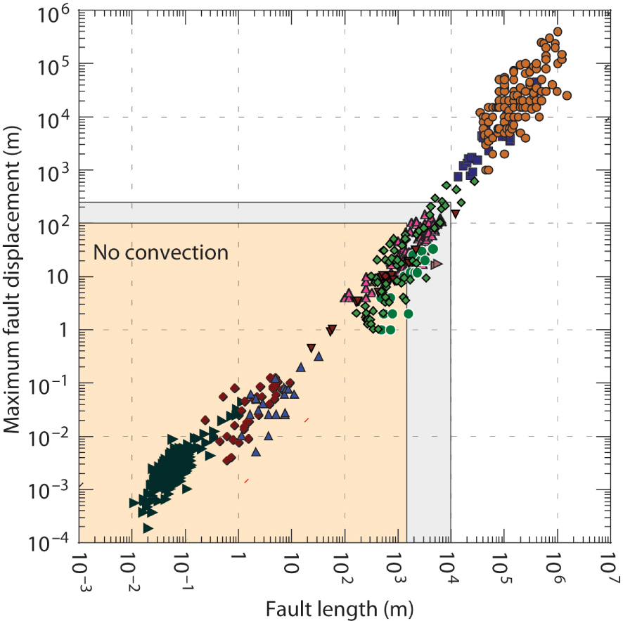
Maximum displacement–length diagram for faults using data from several localities and fault settings [Fossen 2016]. The length of fault associated with displacement in the range of 100–150 m associated with a thickness of damage zone of 100 m or more (see Figure 6) is highlighted in light grey. Areas in light orange correspond to the faults where heat conduction is dominant.
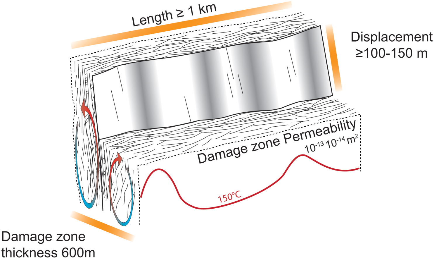
Example of a normal fault with a damage zone thickness of 600 m, where permeability ranges between 10−14 and 10−13 m2. The other geometrical parameters necessary to generate convection cells and high temperatures at shallow depths are indicated [modified after Fossen 2016].
The database of Scibek [2020] contains numerous information on the permeability of fault zones around the world, associated with fault zone parameters available: protolith, kinematic, length, displacement, damage zone thickness. Despite the important number of referenced sites (511 sites), it remains incomplete and spatially distributed in a heterogeneous way. We have sorted the database according to the 3 main fault geometrical criteria to select the sites that can be potential targets for geothermal exploration. The results highlight that one third of the sites (173 sites) have favorable fault geometrical settings for geothermal exploration.
Table 1 shows a selection of a few fault zones, whose length is larger than 1 km, whose displacement is larger than 100 m, and where maximum fault thickness is larger than 150 m. Data belonging to the “Geothermal reservoir” category illustrates some well-known geothermal systems providing several tens of MW (Dixie Valley in Nevada; Kakkonda, Japan; Balçova, Turkey). In the lower half of Table 1, other fault zone categories show cases where permeability is probably sufficiently large because the fault width exceeds several hundreds of meters (Gryphon, Saskatchewan; Eklutna, Alaska). Some systems where permeability is unknown are also indicated since their fault widths approach or even exceed 1 km (Sandwich, Illinois; Carboneras, Spain).
Selection of a few fault zones from the database of Scibek [2020], where fault length is greater than 1000 m, fault displacement greater than 100 m, and fault thickness greater than 150 m
| Site number | Short name | Country/State | Category | Max. thickness (m) | Permeability (m2) | Power production (MWe) | |
|---|---|---|---|---|---|---|---|
| DZ | Bulk | ||||||
| 167 | Chingshui | Taiwan | Geothermal reservoir | 260 | / | 2.5 × 10⁻¹⁴ | 4.2 |
| 180 | Balçova | Turkey | Geothermal reservoir | 1000 | / | 4 × 10⁻¹³ | 72 |
| 139,1 | Ogiri | Japan | Geothermal reservoir | 150 | / | 6 × 10⁻¹³ | 30 |
| 154 | Los Azufres | Mexico | Geothermal reservoir | 1000 | / | 4 × 10⁻¹³ | 161.5 |
| 176 | St Gallen | Switzerland | Geothermal reservoir | 1000 | / | 5 × 10⁻¹⁴ | Abandoned |
| 186 | Dixie | Nevada | Geothermal reservoir | 1000 | / | 10−12 | 70.9 |
| 141,1 | Kakkonda | Japan | Geothermal reservoir | 1000 | / | 2 × 10⁻¹⁴ | 50 |
| 328 | Gryphon | Saskatchewan | Engineering | >500 | 10−15 | / | |
| 370 | Eklutna | Alaska | Engineering | 1000 | / | 3 × 10⁻¹² | |
| 265,1 | Sandwich | Illinois | Groundwater supply | 800 | / | / | |
| 247 | Gloucester | Ontario | Groundwater supply | 300 | / | 2 × 10⁻⁹ | |
| 33,1 | Neodani | Japan | Active fault/processes | 200 | / | 2.3 × 10⁻¹³ | |
| 51 | Lansjärv | Sweden | Active fault/processes | 150 | / | 10−13 | |
| 40,1 | Alpine | New Zealand | Active fault/processes | 100 s | / | 6 × 10⁻¹⁴ | |
| 47 | Carboneras | Spain | Active fault/processes | 2000 | / | / | |
| 55 | San Andreas | California | Active fault/processes | 500 | / | 2 × 10⁻¹⁴ | |
The site number comes from the database. DZ = Damage zone. “Bulk” refers to data that cannot be relocated in fault core or damaged zones. The first 7 lines correspond to geothermal systems for which power production is indicated.
6.4. Potential geothermal systems in European fault zones
At the scale of Europe, fault geometrical parameters applied to the databse of Scibek [2020] highlight 40 fault zones with a favorable geometry for hosting geothermal systems. We also added three crustal fault zones that have been previously mentioned in this study (i.e., the Pontgibaud and Têt fault systems in France, and the fault zone of Larderello in Italy). Fault kinematics are represented in Figure 13a. The maps in Figure 13 show the spatial distribution of geothermal power plants and the selected fault zones with their kinematics (Figure 13a) and with their associated permeabilities (Figure 13b).
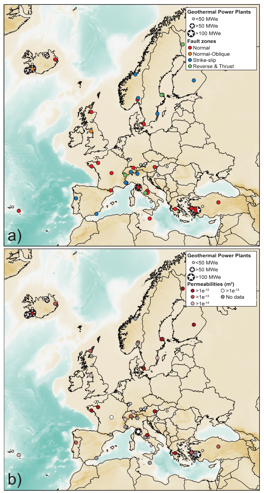
(a) Geothermal fields installed and exploited in Europe (star symbols) (https://www.thinkgeoenergy.com/map/). Selected fault zones from the database of Scibek [2020] with geometrical criteria (length greater than 1000 m, displacements or damage zone thickness greater than 100 m) favorable for geothermal exploration are also indicated. Note the different types of faults. (b) Map showing the main faults permeabilities from the database of Scibek [2020] and geothermal systems. Permeabilities for the Larderello geothermal system and Pontgibaud system are from Bertani and Cappetti [1995] and Duwiquet et al. [2021] respectively. Masquer
(a) Geothermal fields installed and exploited in Europe (star symbols) (https://www.thinkgeoenergy.com/map/). Selected fault zones from the database of Scibek [2020] with geometrical criteria (length greater than 1000 m, displacements or damage zone thickness greater than 100 m) favorable for geothermal ... Lire la suite
Some countries do not contain any new data (Germany, Poland) but this is only due to the lack of geometrical data in the database for these sites. For example, the Unterhaching fault zone [Germany, site number 101.1 in Scibek 2020] would have a high bulk permeability of 10−13 m2, but there is no information on the fault length, displacement or the damage zone thickness. Consequently, these maps must be considered as a first step to define new potential targets for geothermal exploration.
The maps in Figure 13 highlight that only a few fault zones currently host exploited geothermal reservoirs, but some of them control the location of several power plants. This is the case for the Menderes Massif (Turkey) where at least 45 power plants are located close to the low-angle normal fault systems with a total capacity of 1450 MWe. The identified new sites tend to show some similarities even though they are located in different tectonic contexts. Further, these maps show that all tectonic contexts may be interesting, in particular the extensional regime represented by normal faults. However, this may also be due to a bias in the incomplete database. Our selection, based on purely geometrical criteria, shows that fault permeabilities range from 10−15 to 10−12 m2, a favorable range for high-temperature geothermal systems. Based on these observations and criteria, we suggest that the geothermal potential in Europe is still underestimated.
6.5. Perspectives for geothermal exploration in fault zones
Beside being heterogeneous, the Scibek [2020] database lacks numerous permeability data of European fault zones. Consequently, Figure 13 should not be considered as a predictivity map since several additional features must be taken into account before being usable to predict the presence of an exploitable geothermal system. Indeed, information on fault zone geometry and permeability data should be combined with the regional tectonic regime, the local stress field and the surrounding topography. In addition, it is important to recall that the permeability database of fault zones in Europe is not exhaustive, (since in constant evolution). We however believe that our study can help geothermal exploration towards a more efficient targeting, where permeability enhancement techniques would not be necessary.
We focused our study on thermal anomalies greater than 150 °C at a depth lower than 4 km. It must be noted that the recent study by Lund et al. [2022] indicates that “electric power from geothermal energy is now being produced from resources with temperatures as low as 90 °C, using the organic Rankine cycle process in binary power units”. Consequently, our selection must be considered as a lower limit since temperatures around 100 °C at a depth of 1–2 km should be easily found in wide fault zones (Figure 8b), thus increasing the number of fault zones that could be considered as promising targets for geothermal exploration.
Conflicts of interest
Authors have no conflict of interest to declare.
Acknowledgements
This research has been supported by the GERESFAULT project (grant no. ANR-19-CE05-0043-01), GM acknowledges funding from the program TelluS of the Institut National des Sciences de l’Univers, CNRS. Discussions with Patrick Ledru and Vincent Bouchot helped to improve the ideas developed in this study. We thank reviewers Domenico Montanari and Christoph Wanner for their positive and constructive reviews. We also thank Olivier Fabbri for additional suggestions that help to improve the final version of the manuscript.
Appendix A. Numerical modeling: model set-up, equations and physical parameters
All numerical models of this study have been computed with the Comsol Multiphysics™ software. Several different benchmark experiments have been performed, and previously published results were reproduced by our numerical procedure [Eldursi et al. 2009; Garibaldi et al. 2010; Taillefer et al. 2017; Guillou-Frottier et al. 2020; Duwiquet et al. 2022]. Figures 8, 9 and 10 have different model setups and their peculiarities are described below.
A.1. Models of Figure 8
The series of numerical models reported in Figure 8 have been performed in 2D, where a permeable fault zone of variable width and variable permeability is embedded into a low permeable host rock. Model set-up, geometry and boundary conditions are illustrated in Figure A1. Physical properties and other details are also indicated. The heat equation, Darcy law and mass conservation are coupled through the velocity field and the temperature-dependence of fluid properties. An identical numerical procedure as that described in Guillou-Frottier et al. [2020] was used.
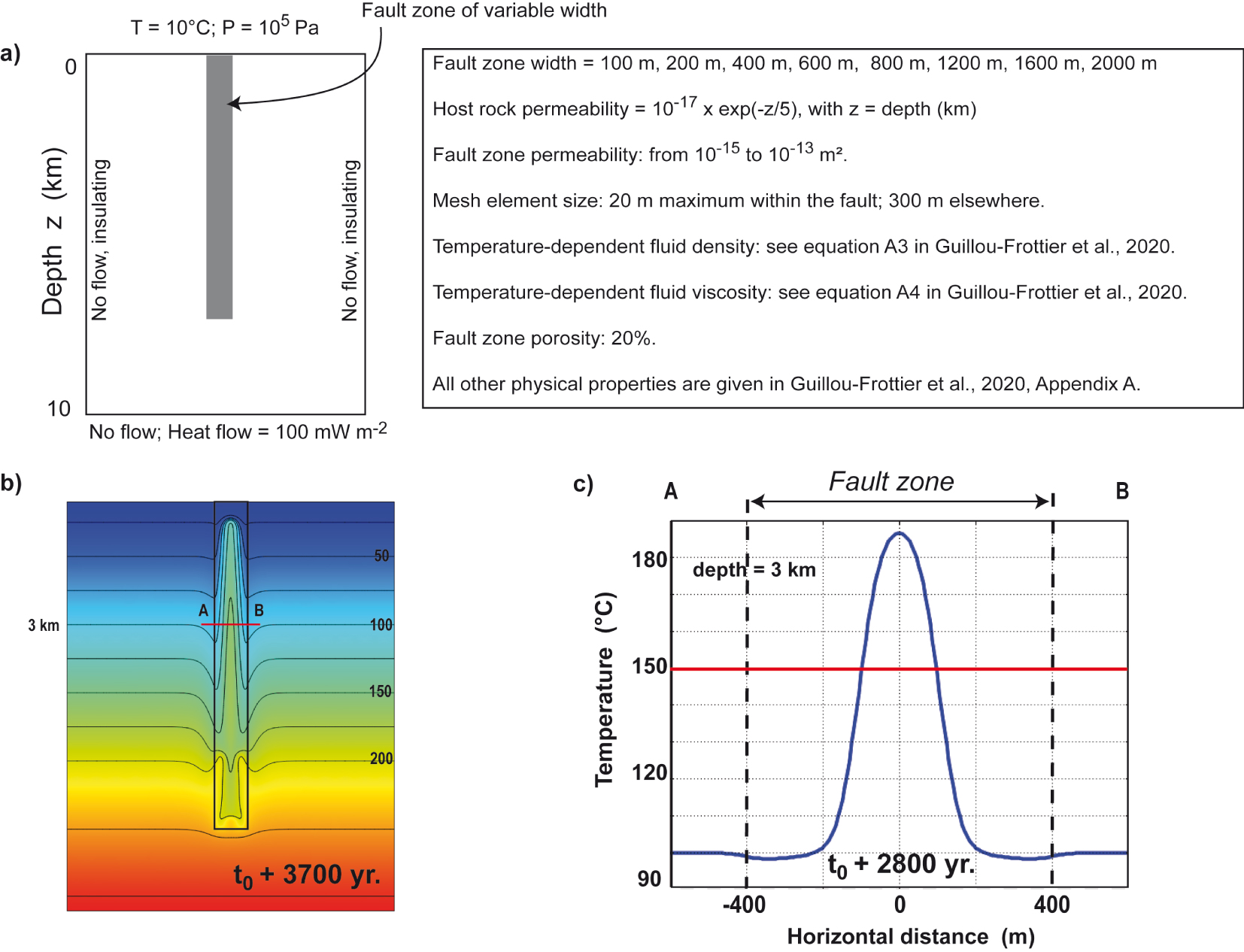
Details on the numerical modeling leading to the results illustrated in Figure 8. For these models, a fixed temperature condition is imposed at the surface. (a) Model set-up, parameters, and boundary conditions; (b) temperature field (isotherms in black contours, separated by 25 °C) for a fault width of 800 m and a fault permeability of 5 × 10⁻¹⁴ m2, 3700 yr after the beginning of the experiment; (c) horizontal temperature profile at a depth of 3 km (profile A–B in b), at the time when temperature perturbation is maximum. Masquer
Details on the numerical modeling leading to the results illustrated in Figure 8. For these models, a fixed temperature condition is imposed at the surface. (a) Model set-up, parameters, and boundary conditions; (b) temperature field (isotherms in black contours, separated by ... Lire la suite
A.2. Models of Figure 9
The models of Figure 9, partly dedicated to the role of topography, account for the altitude-dependence of the surface pressure (see expression p0 and p in Table A1). A mixed thermal boundary condition is imposed at the surface (details below), allowing to get cold temperatures (5–10 °C) at high altitudes, hot temperatures above the fault zone (thermal springs up to 80 °C) and 10 °C elsewhere [see details in Taillefer et al. 2018]. Fluid and rock properties, tested parameters, initial conditions, and boundary conditions are detailed in Table A1. Additional results are shown in Figure A2.
Additional results with horizontal temperature profiles at a depth of 2000 m.
Parameters and variables used in numerical models of Figure 9
| Fluid variables and parameters | |||
| Fluid dynamic viscosity | 𝜇 | 2.414 × 10⁻⁵ exp(570∕((T − 273.15) + 133)), T in K | Pa⋅s |
| Fluid density | 𝜌f | 1036.5 − 0.14167 × (T − 273.15) − 0.0022381 × (T − 273.15) × (T − 273.15), T in K | kg/m3 |
| Thermal capacity | Cpf | 4180 | J/(kg⋅K) |
| Thermal conductivity | 𝜆f | 0.60 | W/(m⋅K) |
| Thermal expansion coefficient | 𝛼 | 10−4 | 1/K |
| Rock variables and parameters | |||
| Mass density | 𝜌s | 2650 | kg/m3 |
| Porosity | 𝜙 | 0.10 | |
| Thermal capacity | Cps | 1000 | K/(kg⋅K) |
| Thermal conductivity | 𝜆s | 2.50 | W/(m⋅K) |
| Thermal expansion coefficient | 𝛽 | 7 × 10⁻⁶ | 1/K |
| Basement permeablity | Kb | 10−16 exp(y−SRE)∕2500 y in m, − 7000 < y < SRE | m2 |
| Core zone permeability | Kc | 10−20 | m2 |
| Damage zone permeability | Kd | 2 × 10⁻¹⁴ | m2 |
| Geometric features (tested parameters) | |||
| Scarp relief elevation | SRE | 200, 1000, 3000 | m |
| Fault dip | FD | 30, 90, 60 | deg |
| Total Damage zone Thickness ( |
DZT | 50, 300, 1000 | m |
| Model variables and parameters | |||
| Ambiant temperature | Text | 20 | °C |
| Heat flow at the model base | Q0 | 0.07 | W/m2 |
| Mixed thermal condition at the model surface | qs | 0.05 × (Text-T), T in °C | W/m2 |
| Initial pressure field | p | 105 × ((1 − 0.006 y/288.15)5.255) + (1000 × 9.8 × (−y)), y in m | Pa |
| Surface pressure | p0 | 105 × ((1 − 0.006 y/288.15)5.255), y in m | Pa |
| Initial temperature field | T | Text + 0.03 × ( − y), y in m | °C |
| Thermal insulation | Lateral boundaries | ||
| No flow conditon | Lateral + model base boundaries | ||
Details on the mixed thermal boundary condition fixed at the topographic surface of the numerical model, issued from Taillefer et al. [2018].
A theoretical constant heat flow q0 = 0.07 W⋅m−2 is imposed at the base of the model. The lateral limits of the model are thermally insulated. In order to allow for temperature variations at the surface (cold areas at high altitudes but also warm zones where hot springs emerge), a mixed thermal boundary condition like the one used in Magri et al. [2015] and Taillefer et al. [2018] is applied to the topographic surface:
| (A1) |
Using this value, the few areas at high altitude (above 2000 m) exhibit low temperatures (5–7 °C) while all other areas show surface temperature of 10 ± 2 °C. The initial conditions for the model are a hydrostatic pressure and a purely conductive thermal state, from which a steady state is computed.
A.3. Models of Figure 10
The numerical procedure for the models of Figure 10, as well as the benchmark for the 3D experiment, have been described in Duwiquet et al. [2022].