





 CC-BY 4.0
1. Introduction
Volcanic systems are complex and evolving geological structures that can pose serious threats to surrounding populations, with approximately 280,000 deaths since the 14th century related to volcanic activity (Brown et al., 2017, and references therein). Monitoring active edifices and detecting unrest periods prior to volcanic eruptions are, therefore, key actions to mitigate risks for populations and properties. This task, performed by various volcano observatories around the world, involves the continuous analysis and interpretation of multiple observables recorded in the field, including seismicity, ground displacements, and the degassing of volatiles such as SO2. Ideally, this task must be performed in (near) real time to detect without delay any change that could indicate the possible occurrence of an eruption (e.g. Sparks, 2003b; Sparks et al., 2012; Neal et al., 2019, and references therein).
In practice, volcano observatories largely rely on seismic activity to monitor the state (rest, unrest or active) of volcanic systems (Sparks et al., 2012). For instance, an increase in volcano-tectonic (VT) seismicity is frequent before eruptions, as observed at Kilauea, Hawaii, USA (e.g. Chastin and Main, 2003) and Piton de la Fournaise, La Réunion island, France (e.g. Collombet et al., 2003). Therefore, tracking the daily number of VT earthquakes provides critical information on the imminence of an eruption, and it can be used to trigger alerts (e.g. at Piton de la Fournaise, see Peltier, Ferrazzini, Di Muro, et al., 2021). Ground displacement data, e.g. from the Global Navigation Satellite System (GNSS) or tiltmeters, can provide further information because they allow for tracking the inflation/deflation of volcanic edifices during periods of unrest and eruption (e.g. Cervelli et al., 2006; Fournier et al., 2009). Combined with physical models, they allow for evaluating the volume and location of magmatic sources at depth (e.g. Mogi, 1958; Dzurisin, 2003; Segall, 2013). Besides, joint analysis of seismicity and ground displacement/deformation data benefits our understanding and monitoring of volcanic systems (e.g., see Peltier, Ferrazzini, Staudacher, et al., 2005; Donaldson et al., 2017; Scarfì et al., 2023). In addition to geophysical signals, monitoring volatile (e.g. CO2 and SO2) concentrations in the soil or in the air provides key information on the degassing state of a volcano and, consequently, on magma storage and circulation at depth (e.g. Sparks, 2003a; Melián et al., 2014; Liuzzo et al., 2015; Boudoire et al., 2017; Moune et al., 2022). In summary, various types of data can be recorded on volcanic edifices, each providing insights into the system’s state at different spatial and temporal scales.
Thanks to its ability to reveal hidden patterns and leverage data statistics, machine learning (ML) may be particularly appropriate for analyzing streams of data produced by volcano observatories. This may help improve volcano monitoring. Application of ML in volcanology has developed rapidly (Whitehead and Bebbington, 2021), particularly for the automatic detection and classification of volcanic earthquakes (Scarpetta et al., 2005; Maggi et al., 2017; Canário et al., 2020; Lapins et al., 2021; Retailleau et al., 2022; Zhong and Tan, 2024) and for refining analyzes of past eruption data (Suarez et al., 2023; Wilding et al., 2023). Although not yet systematically used, ML has also shown promising results in identifying precursory signals and analyzing time series from observatories (e.g., daily VT events, ground displacement) (Luongo et al., 2004; Anzieta et al., 2019; Ren et al., 2020; Dempsey, Cronin, et al., 2020; Zali et al., 2024; Manley et al., 2021; Carbonari et al., 2023; McBrearty and Segall, 2024). ML algorithms have also shown great success in analyzing video data to detect and characterize eruption activity (Corradino et al., 2020; Dye and Morra, 2020; Witsil and Johnson, 2020).
These examples show the increasing use and success of ML in volcano monitoring. However, while seismic signals have been widely investigated, ML applications focusing on processed time series—such as GNSS deformation and VT event counts—remain less explored for volcano state monitoring. Previous ML applications leveraging such time series were mainly used to perform a binary classification of the volcanic state as eruption versus no eruption (Sandri et al., 2004; Brancato et al., 2016; Manley et al., 2021). Another approach is to forecast the future evolution of the deformation and seismicity time series. Volcano observatory staff have strong experience in interpreting such time series, such that having good forecasts could help them better assess the future level of volcanic activity and refine risk assessments by complementing existing alarm systems. Luongo et al. (2004) positively evaluated the ability of artificial neural networks to perform this task for seismicity time series at Vesuvius and ground displacement time series at Phlegraean Fields, Etna and Kilauea, in various states of activity of those volcanic systems. However, the ability of modern ML algorithms to produce reliable forecasts of these time series has not yet been fully tested.
In this study, we evaluate the ability of selected ML algorithms to forecast the VT event count and GNSS deformation time series used for the operational monitoring of Piton de la Fournaise (Morgan, 1971; Peters et al., 2018), an ideal system to develop and evaluate new methods for volcano monitoring (e.g. Maggi et al., 2017; Hibert et al., 2017; Valade et al., 2019; Ren et al., 2020). Indeed, Piton de la Fournaise is very active, with an average of nearly two eruptions per year over the last fifty years, and it has a long history of comprehensive monitoring (Peltier, Chevrel, et al., 2022). It has been monitored since 1979 by a network of monitoring stations (112 as of 2025), among which seismic and GNSS stations (see Figure 1 for a map of the stations used in this study), managed by the Piton de la Fournaise Volcanological Observatory (OVPF-IPGP). By trying to forecast the monitoring signals recorded by OVPF-IPGP, we aim to test (i) whether ML can handle complex volcanic data and identify subtle precursory signals within them, and (ii) whether the operational monitoring signals contain enough information to ensure their self forecasting. The results will allow better understanding if reliable forecasts of time series used for Piton de la Fournaise operational monitoring can be provided to OVPF-IPGP staff to improve volcano monitoring and refine associated risk assessments.
Map of the Enclos-Fouqué caldera, the current most active zone of Piton de la Fournaise. The symbols indicate the location of the seismic and GNSS stations used in this study. The name of the GNSS stations are shown to better highlight the baselines discussed in the text. The green and purple lines indicate the GNSS baselines crossing or surrounding the crater, respectively. Topographic data comes from Litto3D®, a SHOM and IGN project.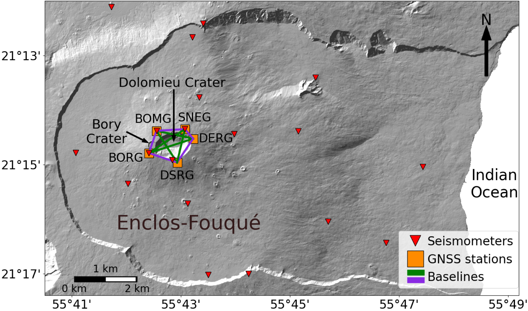
2. Materials and methods
We followed a standard ML time series pipeline, which included (i) data selection, preprocessing, and feature selection; (ii) training different models on a training-validation dataset; and (iii) final evaluation on the test dataset. The models take several original and augmented features as input to forecast their evolution in the future. We evaluated the ability of the models to forecast seismicity or GNSS features, as well as both sets of features. Hereafter, these cases are referred to as the seismicity case, the GNSS case, and the joint case.
2.1. Data
We used seismic and GNSS time series: namely, the daily number of VT earthquakes located below the summit at depths ranging from 2.5 km to the surface (shallow seismicity), and deformation data from the GNSS summit network (Figure 1). These data exhibit long to short term eruptive precursors that help to anticipate the occurrence of eruptions (e.g. Schmid et al., 2012; Peltier, Ferrazzini, Di Muro, et al., 2021, and references therein). During periods of rest, seismicity and deformation are low, with fewer than two VT events per day and ground displacement rates—illustrating the deformation—null or below 0.5 mm per day and showing volcano deflation. When an eruption draws nearer, this pattern changes. Seismic precursors generally appear days to weeks prior to the eruption, as an increase in the number of VT events, from fewer than 5 to more than 50 events per day (Figure 2a,b). GNSS precursors, indicating volcano inflation, also appear generally weeks to months prior to an eruption and consist of ground displacement rates of less than 3 mm per day (Figure 3b). These precursors are generated by the pressurization of the shallowest magma reservoir (around 1.5–2.5 km below the Dolomieu crater, Figure 1) (Peltier, Bachèlery, et al., 2009; Peltier, Villeneuve, et al., 2018; Duputel, Lengliné, et al., 2019).
Daily number of shallow VT earthquakes recorded below Piton de la Fournaise (a) during the 2008–2024 period, with a zoom (b) on the May 1st, 2023 to September 1st, 2023 period that includes the July–August 2023 eruption. The red patches indicate eruptive periods. The blue vertical lines indicate intrusions. The dark arrows indicate days with more than 400 earthquakes. In (b) we observe a typical example of pre-eruptive and eruptive seismicity. Before June 12th (from May 21 to June 11), seismic activity remained low, with an average of 4 earthquakes/day. From June 12 to July 1, the activity increased, reaching an average of 39 earthquakes/day. The activity was then stable until July 2 when the seismic swarm started at 4 a.m. with 1754 earthquakes recorded in one day and 379 within the next 10 days.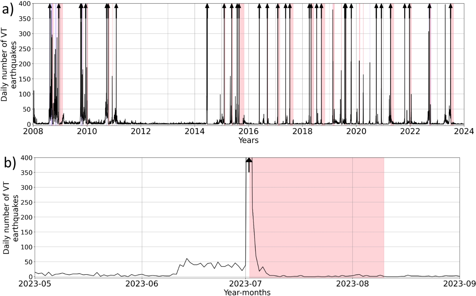
Short-term precursors (from a few minutes to 48 hours) consist of a sharp increase in the number of VT earthquakes, reaching hundreds to thousands of events per hour (Figure 2b). In the same timeline, displacement rates reach several tens of centimeters and sometimes up to more than 1 m in a few hours. These precursors indicate that the magma is ascending from the shallow reservoir to the surface and that an eruption could be imminent (e.g. Collombet et al., 2003; Staudacher and Peltier, 2016; Duputel, Ferrazzini, et al., 2022, and references therein). These windows of increasing seismicity rates, reaching a peak of seismicity, are called seismic swarms. For the monitoring of Piton de la Fournaise, an automatic alarm is raised if the hourly number of VT events reaches a certain threshold, e.g., 3, to alert the OVPF-IPGP staff on duty.
The data used in this study are directly derived from the seismic catalog and displacement GNSS data available through the WebObs monitoring system (Beauducel et al., 2020) used by OVPF-IPGP. For this study, we decided to focus only on data recorded after January 1, 2008, because the activity of Piton de la Fournaise was marked by the 2007 Dolomieu collapse event that significantly affected the deformation behavior of the edifice (Derrien, Peltier, et al., 2020).
As seismicity data, we used the daily number of shallow VT events that occurred between January 1, 2008, and December 31, 2023. This gives us a total of 66,891 earthquakes, covering a total of 62 eruptions or intrusions (i.e. magma injections that did not reach the surface) (Figure 2).
As deformation data, we used the daily evolution of ten baselines (distances between pairs of GNSS stations) calculated using the five GNSS stations located at the summit around the Bory and Dolomieu craters (BOMG, SNEG, DERG, DSRG, and BORG; Figure 1). GNSS baselines are used to reveal subtle deformation as at Piton de la Fournaise displacements are very small prior to an eruption; using baselines allows the removal of noise and significantly increases the signal-to-noise ratio. The evolution of baselines over time shows a clear upward trend (Figure 3). Over 16 years, some baselines have accumulated more than 2 meters of elongation, as observed for DSRG-SNEG (Figure 3b). These long-term trends could introduce biases into ML algorithms and should be removed (Hyndman, Athanasopoulos, et al., 2024). To do so, we computed the gradients of the baselines (Figure 3c), as is sometimes done in volcano monitoring (Fournier et al., 2009).
(a) Baselines (distances between pairs of GNSS stations) calculated using the five summit GNSS stations (BOMG, SNEG, DERG, DSRG and BORG, see also Figure 1 for position and color code). (b) Zoom on the SNEG-DSRG baseline before, during and after the July–August 2023 eruption. (c) Example of the signal we used as input, namely the gradients, with data from the SNEG-DSRG baseline. On the Y -axis labels, 5, 10 and 30 days refer to time window lengths used for gradient computation. The red areas indicate eruptive periods. The blue lines indicate intrusions.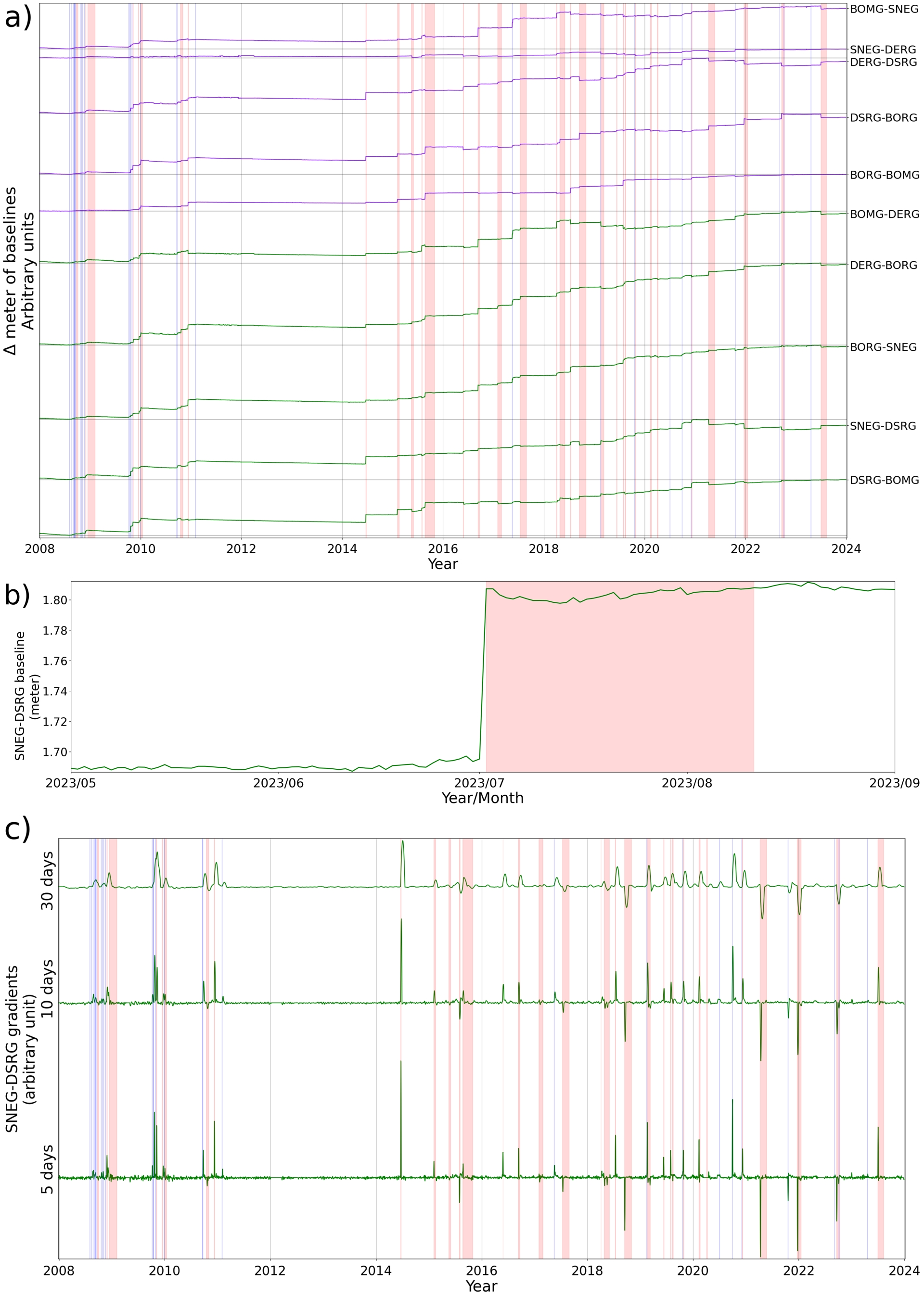
2.2. Feature engineering
As the daily seismicity can span from 0 to more than 1000 VT earthquakes per day (Figure 2), we used its log10 transformation, with NaN values (coming from the log10 of days with 0 events) replaced by 0. Then, to improve model accuracy, we performed feature augmentation (Antwarg et al., 2023). We computed the gradients of the daily log10 number of VT events using windows of 5, 10 and 30 days. These values were chosen to provide gradients on short, moderate, and long timescales. For seismicity, the four features used as input for ML algorithms are thus the daily log10 number of VT events and the gradients of the past 5, 10 and 30 days.
For the GNSS case, we computed three time series gradients for each baseline (10 in total, Figure 3a) using time windows containing the 5, 10 and 30 past days (Figure 3c). Again, these values were selected to provide gradients that are consistent with the different time scales of typical GNSS precursors at Piton de la Fournaise (Figure 3). We did not include the non-gradient baselines in the final dataset, which totals 30 features.
Finally, for the joint case, we used as features the gradients of the past 5, 10 and 30 days of GNSS baselines as well as the daily log10 number of VT events and its gradients for the past 5, 10 and 30 days.
2.3. Preprocessing
We split the seismicity and GNSS time series to have approximately 70, 15 and 15% of the data in the training (1/01/2008–14/03/2019), validation (14/03/2019–6/08/2021), and test (6/08/2021–30/12/2023) sets, respectively. Then, we scaled the time series to ensure the good performance of the ML algorithms. All the original features are centered at 0 but can present large deviations. Therefore, we adopted a simple scaling approach: we divided each feature by its standard deviation calculated using the training data subsets.
2.4. Models
We selected six models, implemented using the Keras and Tensorflow libraries (Martín et al., 2016) in the Python language (van Rossum, 1995), to forecast the time series, including four artificial neural networks (ANNs):
- Last model: this reference deterministic model repeats the last input values.
- Linear model: a linear regression model.
- Dense model: a feed-forward neural network with fully connected layers (Goodfellow et al., 2016), each hidden layer, except the last one, having a non-linear activation function.
- Conv model: a convolutional neural network (CNN). CNNs are similar to feed-forward dense neural networks in that they are composed of layers of interconnected nodes, but they differ fundamentally in how they process data. Rather than considering every input feature simultaneously as in dense networks, CNNs use convolutional layers that scan local regions of the data using learnable filters, known as convolutional kernels. This approach allows CNNs to apply the same set of weights over different regions, capturing important spatial or temporal patterns in the input. The use of convolutional filters is central to their design and gives the model its name. Developed for image analysis tasks, CNNs have also been applied successfully to time series forecasting (Borovykh et al., 2019; Lara-Benítez et al., 2021; M. Liu et al., 2022) and other domains, thanks to their ability to extract local features.
- LSTM model: a Recurrent Neural Network (RNN), using Long Short-Term Memory (LSTM) layers as the core recurrent component and a final linear layer for output (Hochreiter and Schmidhuber, 1997). Those models are designed to handle sequential data such as text or time series (Hochreiter and Schmidhuber, 1997; Lara-Benítez et al., 2021), making them well-suited for forecasting tasks involving temporal dynamics. LSTM layers process inputs iteratively, updating their internal memory (also called the hidden state). At each time step, the network receives the current input along with the previous hidden state, updating its memory and making predictions. This process continues sequentially for each time step in the series. While traditional RNNs often struggle with retaining information over long sequences due to issues like vanishing or exploding gradients (Bengio et al., 1994), LSTMs mitigate these problems through specialized mechanisms called gates—input, forget and output gates—which regulate how information is stored, updated, and output. These gates allow LSTMs to capture longer-term dependencies in data and reduce information loss compared to standard RNNs.
- Transformer model: a Transformer-based model, originally designed for natural language tasks (Vaswani et al., 2017) but now widely used for time series forecasting thanks to its efficiency and scalability. Unlike RNNs, Transformers process sequences in a single forward pass using self-attention (ibid.), enabling rapid training and the modeling of both short- and long-range dependencies. Key mechanisms, such as multi-head attention, positional encoding, and residual connections, help capture complex temporal relationships. Recent adaptations include Informer, FEDformer, TimeGPT-1, and iTransformer (H. Zhou et al., 2021; T. Zhou et al., 2022; Garza and Mergenthaler-Canseco, 2023; Y. Liu et al., 2024). They demonstrate strong forecasting performance on time series data. Here, we implemented a custom version of an encoder-only autoregressive model that was built starting from the code of the Keras tutorial (Ntakouris, 2021). Data is first projected into an embedding space using a linear layer, followed by the addition of a learned absolute positional encoding. The embedded sequence is then processed by a multi-head attention layer, which incorporates two 1D convolutional layers to capture local temporal patterns. This produces a context vector that is passed to an autoregressive decoder. The decoder takes the last time step of the input sequence, embeds it using the same linear embedding layer, sums it with the encoder-provided context, and passes the result through a feed-forward network to predict the next time step. Predicted values are stored and fed back into the decoder for subsequent autoregressive forecasting.
2.5. Performance metrics
Performance of ML models in regression tasks is usually evaluated using the Mean Squared Error (MSE), the Mean Absolute Error (MAE) and the coefficient of determination R2 (Goodfellow et al., 2016). However, in the case of volatile time series, other metrics may be more appropriate (e.g. Hyndman and Koehler, 2006).
To capture the general ability of an ML model to forecast time series, we used the Mean Absolute Scaled Error (MASE) proposed by Hyndman and Koehler (ibid.):
| \begin {equation} \mathrm {MASE} = \frac {({1}/{N})\sum _{t=1}^N |y_t - \hat {y}_t|}{({1}/{N-1})\sum _{t=2}^N |y_t - y_{t-1}|}, \label {eq:MASE} \end {equation} | (1) |
To capture model errors during those bursts due to magma injections leading to eruptions and intrusions, we added a weight to the RMSE to create a peak-weighted Root-Mean-Squared-Error (pRMSE):
| \begin {equation} \mathrm {pRMSE}_{\alpha ,q} = \sqrt { \frac {\sum _{t=1}^N w_t \, (y_t - \hat {y}_t)^2}{\sum _{t=1}^N w_t} }, \label {eq:pRMSE} \end {equation} | (2) |
| \begin {equation} w_t = 1 + \alpha \cdot \mathbf {1}\{\, y_t > Q_{q}(y)\,\}, \end {equation} | (3) |
To facilitate model selection, we used a composite performance metric that combines pRMSE and MASE. It is computed as the sum of each metric divided by its respective median value across all models. With $\overset{\sim }{\mathrm{pRMSE}}$ and $\overset{\sim }{\mathrm{MASE}}$ the median values for all models, one would calculate the Final Score for one model as:
| \begin {equation} \text {Final Score} = \frac {\mathrm {pRMSE}}{\overset {\sim }{\mathrm {pRMSE}}} + \frac {\mathrm {MASE}}{\overset {\sim }{\mathrm {MASE}}} . \label {eq:finalscore} \end {equation} | (4) |
Finally, we also calculated the coefficient of determination R2:
| \begin {equation} R^2 = 1 - \frac {\sum _{t=1}^N (y_t - \hat {y}_t)^2}{\sum _{t=1}^N (y_t - \bar {y})^2}, \label {eq:R2} \end {equation} | (5) |
2.6. Model hyper-parameters
Model hyper-parameter tuning involved both data and model structure optimization. For the data, it included the window size of the input time series. For the models, it included the number of hidden layers and activation units in the ANNs, the number of filters per convolutional layer, the size of the convolutional kernel in CNNs, the use of pooling layers, and the dropout rates (Srivastava et al., 2014). The learning rates for optimization algorithms such as ADAM (Kingma and Ba, 2014) were also tuned. These were tuned to achieve the best possible performance in the training and validation data subsets while having simple, relatively shallow models for this study. Tuning was performed manually for the simple models (e.g. Dense) and automatically using Optuna (Akiba et al., 2019) for the Transformer. Optuna also was used to tune the input time series window size.
2.6.1. Seismicity case
We chose to forecast the signals using a horizon of 5 days (i.e., we forecast the signals for the next 5 days). In general, results are better with a shorter forecasting horizon, as variations tend to increase over time, making predictions more challenging. However, our goal here was to document how ML actually performs in predicting these signals in the future, ideally with the longest possible forecast. Therefore, a 5-day horizon seemed like a reasonable choice. The number of past time steps provided in the inputs of the ML algorithms was tuned using Optuna. Using a value of 16 past time steps yielded the best results.
The hyperparameters of the different ANN models were set as follows:
- Dense: 1 hidden layer with 64 activation units and swish activation functions (Ramachandran et al., 2017).
- Conv: 1 convolutional layer with 32 kernels of size 5 and swish activation functions, followed by a linear output layer.
- LSTM: 1 hidden LSTM layer with 256 activation units and tanh activation functions, followed by a linear output layer.
- Transformer: 1 encoding block with 7 attention heads, a head size of 24, and 200 filters in the hidden 1D CNN layer. The decoder network is composed of one hidden layer with 256 units with a 0.45 dropout rate and swish activation functions.
2.6.2. GNSS case
Automatic tuning with Optuna determined that using 6 past days as input time steps was optimal for forecasting signals over the next 5 days. This number of input time steps may seem short compared to the typical timescale of volcanic behavior, which ranges from weeks to months during unrest periods. However, magmatic injection develops in only a few hours, sometimes less. Moreover, the inputs already contain gradients calculated over the last 5, 10 and 30 days, thus capturing information from the last 30 days. This may explain the better performance of models trained on relatively short sequences.
The hyperparameters of the different models were set as follows:
- Dense: 1 hidden layer with 1024 activation units and swish activation functions.
- Conv: 1 hidden convolutional layer of 256 kernels of size 3 with swish activation functions, followed by a linear output layer.
- LSTM: 1 hidden LSTM layer with 256 activation units and tanh activation functions, followed by a linear output layer.
- Transformer: 1 encoding block with 9 attention heads, a head size of 72, and 8 filters in the hidden 1D CNN layer. The decoder network is composed of one hidden layer with 384 units, a 0.05 dropout rate, and swish activation functions.
2.6.3. Joint case
Automatic tuning with Optuna yielded a best value of 6 past days. The hyperparameters of the different ANN models were set as follows:
- Dense: 1 hidden layer with 1024 activation units and swish activation functions.
- Conv: 1 convolutional layer of 256 kernels of size 3 and swish activation functions, followed by a linear output layer.
- LSTM: 1 hidden LSTM layer with 256 activation units and tanh activation functions, followed by a linear output layer.
- Transformer: 1 encoding block with 11 attention heads, a head size of 56, and 8 filters in the hidden 1D CNN layer. The decoder network is composed of one hidden layer of 512 units with a dropout rate of 0.45 and swish activation functions.
2.7. Training procedure
Models are trained through gradient descent by backpropagation (Rumelhart et al., 1986) using the Adam optimizer (Kingma and Ba, 2014) to minimize Huber loss (Huber, 1964) between observed and predicted future values. We tested various loss functions, and Huber loss performed best. The learning rates were set to starting values of 0.1, 0.01, or 0.001, depending on the model, and were further optimized using Optuna for the Transformer model. Learning rate decay (Chollet et al., 2023; Wu and L. Liu, 2023) was further applied with a patience of 5, and a decay rate value between 0.5 and 0.9 optimized using Optuna. We used early stopping to end the model’s training when the loss on the validation set stopped decreasing after 15 epochs. Only the models with the best validation scores were saved for future evaluation.
To assess how model initialization and training variability affect the distribution of predictions—without greatly increasing computational cost—we trained 10 instances of each architecture—the Linear model and the four ANN variants—using different random seeds for each set. For consistency, the same seeds were applied across all architectures.
3. Results
We first evaluated the performance of the models separately on the seismicity and GNSS datasets. We measured which model performed the best and reported on its ability to forecast future data. Next, we repeated this process and evaluated if combining the seismicity and GNSS datasets yielded better results in forecasting the time series.
3.1. Seismicity case
All models outperform the Last method for predicting the seismic time series (Table 1). Train, validation, and test metrics are relatively similar, indicating that we did not overfit the dataset. On the test dataset, the Transformer method performs the best according to the Final Score. It also presents the best Test R2. Using non-linear methods tends to improve model forecasting abilities. After the Last method, the method presenting the worst metrics is the LSTM one.
Seismicity case: Peak-weighted Root Mean Squared Error (pRMSE, Equation (2)), Mean Absolute Scaled Error (MASE, Equation (1)), Coefficient of determination (R2, Equation (5)), and Final Score (Equation (4)) calculated using predictions from 10 different runs per model
| Model | Train pRMSE | Valid. pRMSE | Test pRMSE | Train MASE | Valid. MASE | Test MASE | Train R2 | Valid. R2 | Test R2 | Final Score |
|---|---|---|---|---|---|---|---|---|---|---|
| Last | 0.361 | 0.419 | 0.348 | 1.63 | 1.63 | 1.71 | 0.420 | 0.253 | 0.394 | 2.393 |
| Linear | 0.3160(11) | 0.3700(5) | 0.3117(9) | 1.279(10) | 1.245(10) | 1.355(12) | 0.6005(11) | 0.472(2) | 0.5685(10) | 2.014 |
| Dense | 0.298(3) | 0.375(3) | 0.3032(19) | 1.222(10) | 1.241(12) | 1.337(14) | 0.655(6) | 0.474(7) | 0.587(3) | 1.972 |
| Conv | 0.306(3) | 0.3740(18) | 0.306(3) | 1.240(9) | 1.229(14) | 1.341(14) | 0.637(5) | 0.479(3) | 0.585(6) | 1.986 |
| LSTM | 0.297(9) | 0.377(5) | 0.318(8) | 1.27(4) | 1.35(5) | 1.50(6) | 0.660(16) | 0.469(11) | 0.543(18) | 2.137 |
| Transformer | 0.2987(16) | 0.3612(20) | 0.292(2) | 1.245(10) | 1.234(11) | 1.342(19) | 0.656(5) | 0.508(3) | 0.618(6) | 1.941 |
Best scores per metric are marked in bold.
The forecasting performance of the models over the 5 days horizon reveals a systematic pattern. Predictions at t + 1 day (next day prediction) are much better than those at t + 5 days (Figure 4). All the ML models present pRMSE around 0.26 at t + 1 day. This value quickly and steadily increases as the forecast horizon extends. The most complex model, Transformer, presents the best overall variations in pRMSE as a function of the prediction time step. Although at t + 1 day its performance is similar to that of other non-linear models, the decrease in its forecasting accuracy (here measured by pRMSE) is less pronounced than those of other models as the prediction time step increases. It seems that the complexity of the Transformer model gives a little edge in handling more complex predictions. Based on these observations, model predictions are, on average, quite accurate for the next two days but rapidly degrade when attempting to predict further ahead.
Seismicity case: Peak-weighted Root-Mean-Squared-Error pRMSE as a function of the prediction time. Lower is better. pRMSE is calculated using the predictions of 10 models. Dashed lines are guides for the eyes.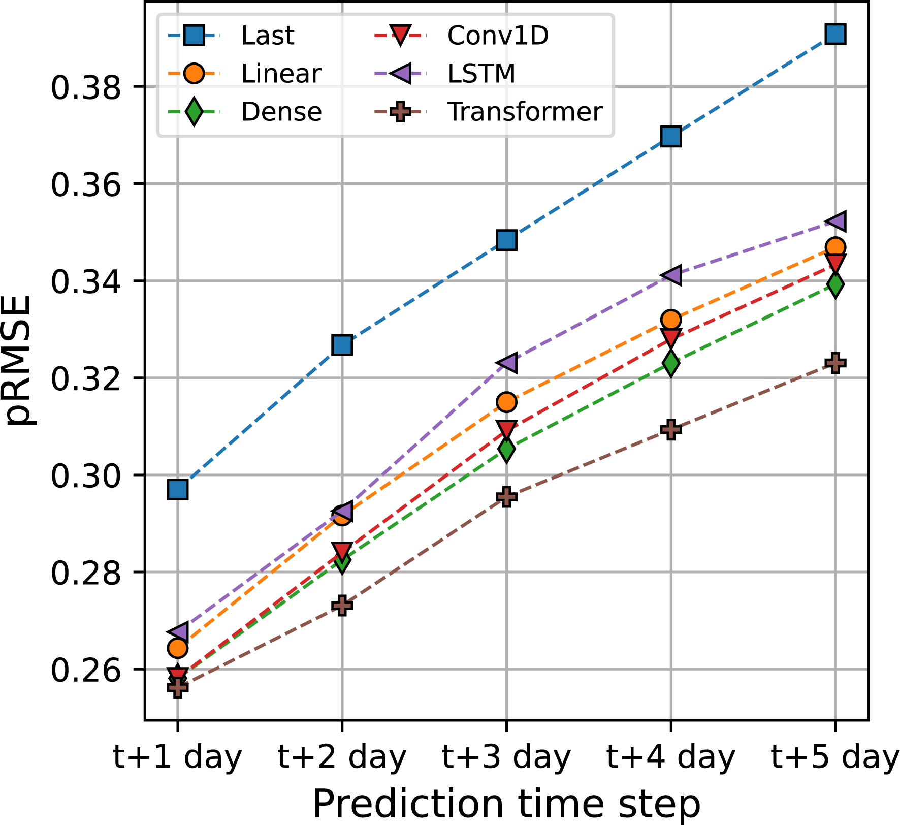
The models we tested forecast all the features passed as inputs. This allows for observing how well they perform in forecasting the different features (Figure 5). pRMSE values for the daily seismicity predictions (all time steps) range between 0.45 and 0.55, with the best performing model being the Transformer. pRMSE scores on the 5, 10 and 30 day gradients are significantly lower. All models better forecast those features because calculating gradients tends to smooth the signals. The higher the gradient calculation window, the smoother the final feature, making them easier to forecast.
Seismicity case: Peak-weighted Root-Mean-Squared-Error pRMSE per feature. Lower is better. pRMSE is calculated using the predictions of 10 models.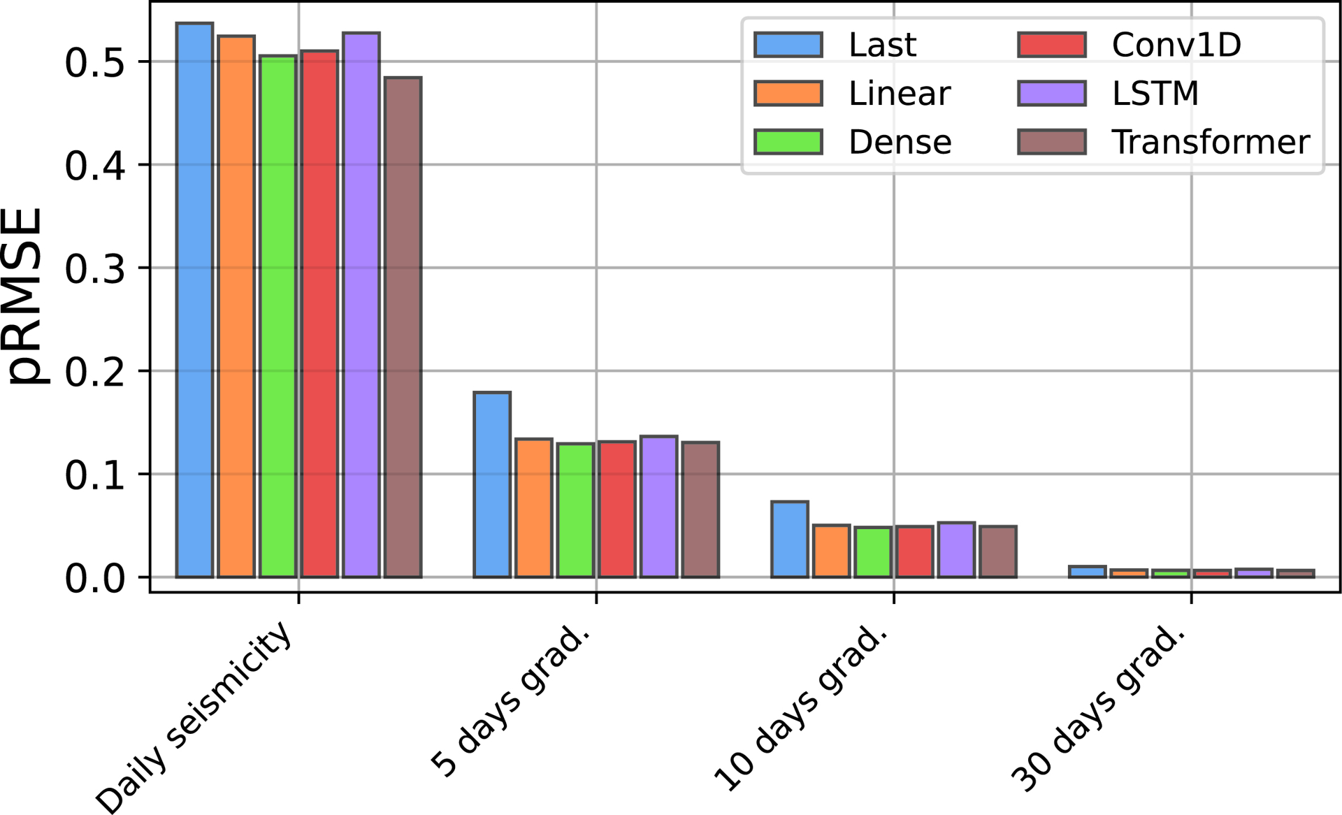
To better understand the forecasting behavior of the models, we compared predictions from the best-performing Transformer method and the data (Figure 6) for the June–August 2023 time window, during which an eruption started on July 2, 2023. For the daily seismicity (Figure 6a), although next-day predictions match the data trend well, a lag of one day is observed, and the peak on July 2 is not well reproduced. This indicates that the model reacts to changes in the dataset, particularly when seismicity is increasing abruptly. This is clearly visible during the June 7 to 16 and July 1 to 7 periods. At the start of those periods, the full 5-day forecasts always show constant or slightly decreasing trends (gray lines in Figure 6). Forecasts are much better when the daily VT seismicity is constant or decreasing. Indeed, decreases in seismicity are well predicted (see in particular the period from July 4 to July 13 in Figure 6).
Seismicity case: Comparison between data (black line) and forecasts (blue dots) from a Transformer model for the number of VT events per day in log10 units (a) and its gradient at 5, 10 and 30 days (panels b, c, d, respectively). The blue dots are the forecasts for the next day, and the lines attached to them represent the full 5-day forecast. We focus here on the period between June 1 and August 1, 2023, during which an eruption started on July 2.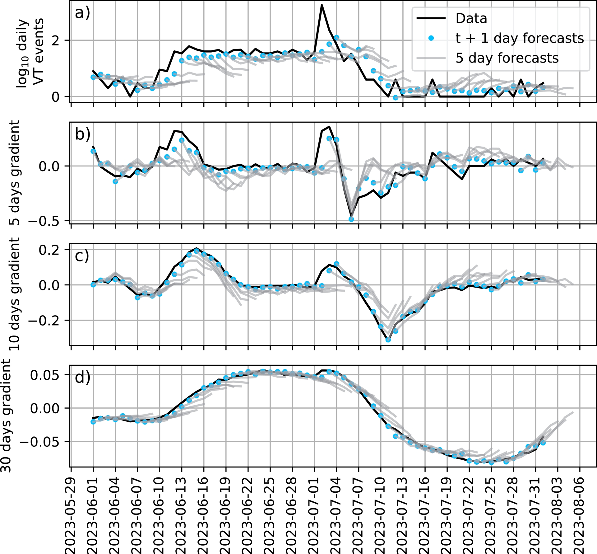
Forecasts are better for the 10 day gradient (Figure 6b). A forecast lag is sometimes observed (e.g. between June 7 and 14), but it is not systematic. Results further improve for the 30 day gradient, as testified by good metrics (e.g. Figure 5). This is probably due to the smoothness of long-term gradients, making them much easier to forecast than the volatile daily VT seismicity. We report here only the results for a Transformer model for the sake of brevity, but other models show similar or worse behavior.
3.2. GNSS case
Taking into account pRMSE and R2, all ML models perform better than the Last method (Table 2). However, only the Linear model outperforms Last according to the MASE and Final Score values. The ML models are thus not performing well on this dataset.
GNSS case: Peak-weighted Root Mean Squared Error (pRMSE, Equation (2)), Mean Absolute Scaled Error (MASE, Equation (1)), Coefficient of determination (R2, Equation (5)), and Final Score (Equation (4)) calculated using predictions from 10 different runs per model
| Model | Train pRMSE | Valid. pRMSE | Test pRMSE | Train MASE | Valid. MASE | Test MASE | Train R2 | Valid. R2 | Test R2 | Final Score |
|---|---|---|---|---|---|---|---|---|---|---|
| Last | 0.004 | 0.003 | 0.003 | 2.44 | 2.39 | 2.28 | −0.038 | −0.022 | −0.102 | 1.957 |
| Linear | 0.0032(19) | 0.0027(13) | 0.0022(5) | 2.01(3) | 1.991(15) | 1.968(11) | 0.5038(3) | 0.5044(4) | 0.4734(4) | 1.626 |
| Dense | 0.0031(3) | 0.0028(10) | 0.0023(9) | 2.56(9) | 3.22(7) | 3.03(12) | 0.516(9) | 0.422(3) | 0.366(7) | 2.059 |
| Conv | 0.0031(2) | 0.0028(11) | 0.0023(18) | 2.55(9) | 2.99(8) | 2.92(12) | 0.512(8) | 0.437(4) | 0.379(12) | 2.018 |
| LSTM | 0.0033(8) | 0.0030(3) | 0.0025(18) | 2.62(6) | 3.36(7) | 3.06(8) | 0.47(3) | 0.343(12) | 0.260(10) | 2.158 |
| Transformer | 0.0032(2) | 0.0029(13) | 0.0024(14) | 2.49(16) | 2.76(10) | 2.71(17) | 0.483(8) | 0.399(4) | 0.353(6) | 1.978 |
Best scores per metric are marked in bold.
The per-day pRMSE scores of the models show variations similar to those previously seen for the seismicity case (Figure 7). The Linear model performs well with a pRMSE of 0.001 at t + 1 day. As we expand the forecasting horizon to t + 5 days, the forecast quality of all models decreases rapidly. Based on those observations, forecasts from the Linear model are on average relatively accurate for the next two days, and forecasting quality rapidly degrades when attempting to predict further ahead.
GNSS case: Peak-weighted Root-Mean-Squared-Error pRMSE as a function of the prediction time. Lower is better. pRMSE is calculated using the predictions of 10 models. Dashed lines are guides for the eyes.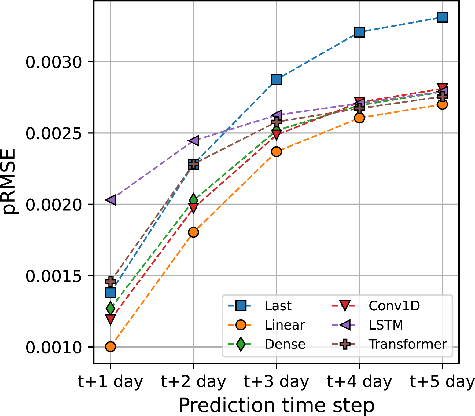
The best performing Linear model reproduces not very well the GNSS 5 day gradients (Figure 8), probably due to their high volatile character. Gradients at 10 days are better reproduced, as indicated by significantly lower pRMSE. This is further true for the gradients at 30 days, which are even better reproduced, with pRMSE values lower than 0.001. Other models show a similar pattern (not shown). Models thus have difficulties forecasting noisy GNSS variations at short time scales and perform better for the prediction of long-term trends. This is because GNSS variations mostly occur slowly on a long-term scale or rapidly over a very short time period of less than 1 day, so often displacements can be too subtle to distinguish from noise. We finally observe that, at a given gradient time window, pRMSE values vary significantly between the different GNSS baselines.
GNSS case: Peak-weighted Root-Mean-Squared-Error pRMSE per feature. Lower is better. pRMSE is calculated using the predictions of 10 Linear models.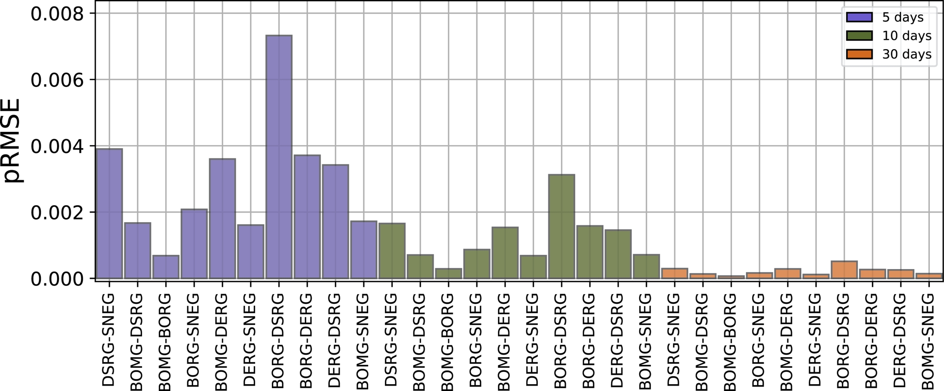
Visual inspection of the GNSS forecasts reveals that the results are actually better than what is inferred from the overall performance metrics. For the DSRG-SNEG baseline (Figure 9), t + 1 day forecasts are consistent with the 5 day gradient values around the July 2023 eruption, and fall very close to the values of the gradients at 10 and 30 days. In particular, 5 day forecasts are consistent with the overall shape of the data (gray lines in Figure 9) except right before the start of the eruption on July 2, 2023. Indeed, the model does not forecast the incoming sharp increase in deformation generated by the magma injection that fed the eruption. However, once the fast deformation starts, forecasts of the deformation during and after the eruption are better.
GNSS case: Comparison between data (black line) and forecasts (blue dots) from a Linear model for the DSRG-SNEG baseline gradients at (a) 5 days, (b) 10 days and (c) 30 days. The blue dots are the forecasts for the next day, and the lines attached to them represent the full 5-day forecast. We focus here on the period between June 1 and August 1, 2023, during which an eruption started on July 2.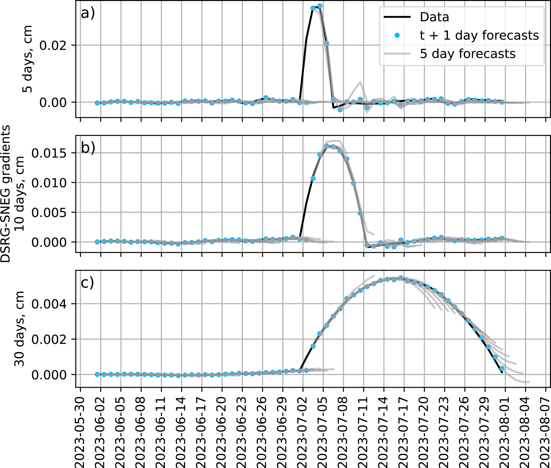
3.3. Joint case
To assess whether there is any gain in combining seismicity and GNSS data for performing forecasts, we trained the models on the combined seismic and GNSS features. As for the GNSS case, pRMSE and R2 values suggest that all machine learning models substantially outperform the Last baseline (Table 3), but MASE and Final Score values yield a more mitigated pattern. Indeed, taking into account those metrics, only Linear outperforms Last. This suggests that the gain in variance explanation and in reproduction of sharp signal bursts provided by models such as LSTM or Transformer partly comes at the cost of overall robustness. Similarly to what has been observed in Section 3.2, Linear also presents overall good performances when looking at pRMSE per prediction time step (Figure 10).
Joint case: Peak-weighted Root Mean Squared Error (pRMSE, Equation (2)), Mean Absolute Scaled Error (MASE, Equation (1)), Coefficient of determination (R2, Equation (5)), and Final Score (Equation (4)) calculated using predictions from 10 different runs per model
| Model | Train pRMSE | Valid. pRMSE | Test pRMSE | Train MASE | Valid. MASE | Test MASE | Train R2 | Valid. R2 | Test R2 | Final Score |
|---|---|---|---|---|---|---|---|---|---|---|
| Last | 0.130 | 0.148 | 0.124 | 2.34 | 2.30 | 2.21 | 0.461 | 0.309 | 0.431 | 1.930 |
| Linear | 0.1138(3) | 0.1345(4) | 0.1117(3) | 2.15(4) | 2.07(3) | 2.16(3) | 0.6396(9) | 0.4861(10) | 0.6007(16) | 1.802 |
| Dense | 0.1082(7) | 0.138(2) | 0.1144(16) | 2.45(11) | 2.95(5) | 2.92(11) | 0.683(4) | 0.455(13) | 0.556(16) | 2.109 |
| Conv | 0.1096(7) | 0.1375(16) | 0.113(2) | 2.50(8) | 2.86(4) | 2.82(7) | 0.674(4) | 0.475(11) | 0.586(16) | 2.063 |
| LSTM | 0.1076(9) | 0.138(3) | 0.1099(11) | 2.69(4) | 3.46(4) | 3.32(6) | 0.691(6) | 0.459(13) | 0.621(5) | 2.223 |
| Transformer | 0.1139(7) | 0.1381(11) | 0.1125(9) | 2.33(9) | 2.51(6) | 2.50(8) | 0.654(5) | 0.464(11) | 0.614(5) | 1.937 |
Best scores per metric are marked in bold.
Joint case: Peak-weighted Root-Mean-Squared-Error pRMSE as a function of the prediction time. Lower is better. pRMSE is calculated using the predictions of 10 models. Dashed lines are guides for the eyes.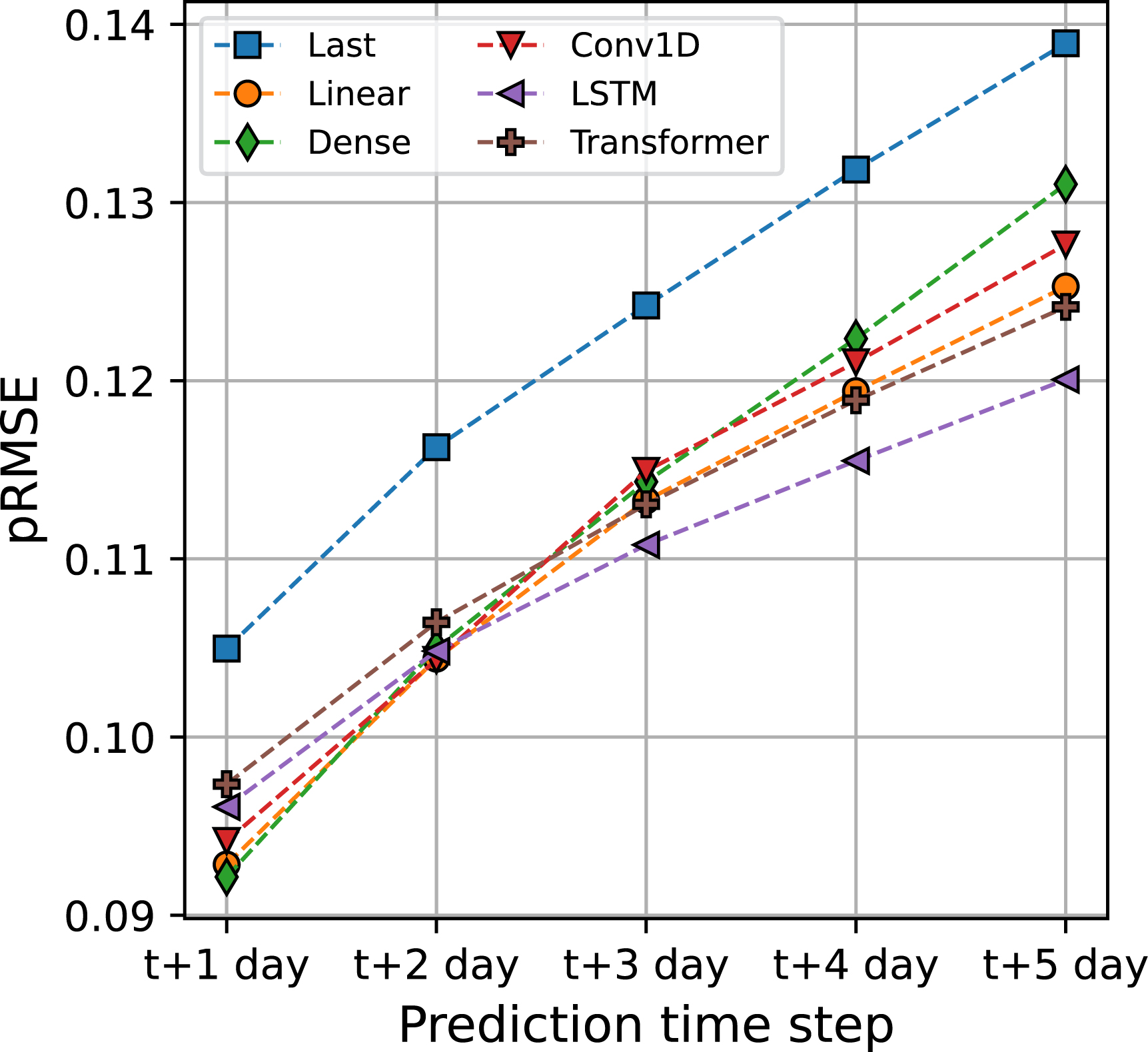
The central question at this point is: does combining the seismicity and GNSS datasets provide any edge for producing better forecasts? To answer this question, we plot the histograms of the relative change in per-feature pRMSE for the best models trained on the seismicity (Transformer), GNSS (Linear) and joint datasets (Linear) in Figure 11. Compared to the models trained on separate datasets, those trained on the joint dataset yield limited improvements for forecasting some seismicity features and perform worse on the GNSS features (Figure 11). Therefore, in the present context, combining the seismicity and GNSS datasets provides limited complementary information for forecasting.
Observing the forecasts from the best-performing Linear model reinforces the idea that combining the seismicity and GNSS datasets provides no clear gain (Figure 12). Focusing again on the July–August 2023 eruption, seismicity features are in general slightly better predicted (Figures 6, 12a,b,c,d), as expected from pRMSE comparison (Figure 11). A 1-day lag is still observed, indicating that the model reacts to changes and does not truly forecast them. However, GNSS forecasts are also not as good as those performed by the Linear model trained only on GNSS data (Figures 9, 12e,f,g). In addition, forecasts still do not reproduce the increase in deformation on July 2, 2023 just before the start of the eruption.
Comparison of forecast performance using separate versus joint datasets. Histograms show the relative change in peak-weighted RMSE (pRMSE) for GNSS features (green) and seismicity features (olive) when using joint datasets versus separate datasets. The best models for each case were used to generate the predictions (see text).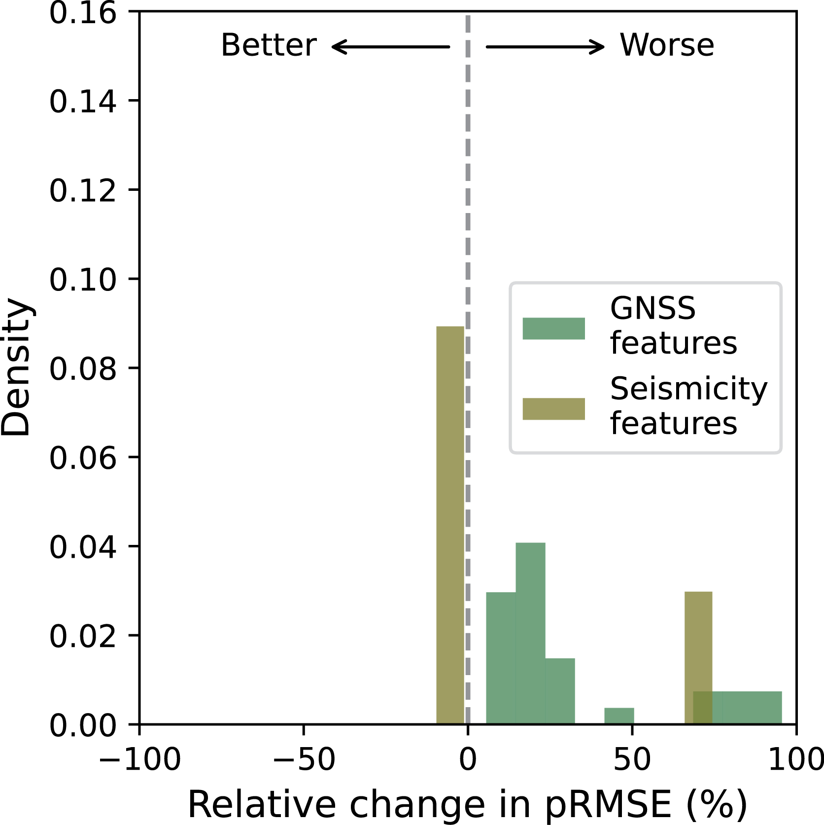
Joint case: Comparison between data (black line) and forecasts (blue dots) from a Linear model for daily seismicity features (a–d) and the DSRG-SNEG baseline gradients (e–g) at 5 days, 10 days and 30 days. The blue dots are the forecasts for the next day, and the lines attached to them represent the full 5-day forecast. We focus here on the period between June 1 and August 1, 2023, during which an eruption started on July 2.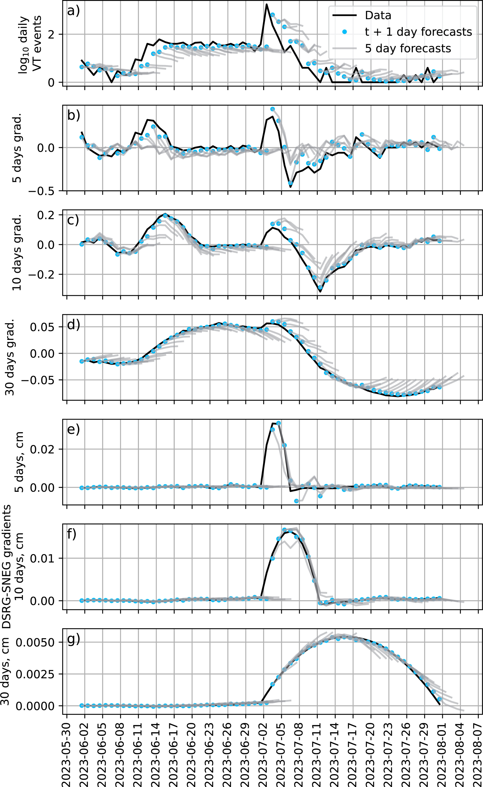
4. Discussion
The goal of this work was to assess how well different machine learning models can forecast seismic and deformation time series used by OVPF-IPGP for monitoring Piton de la Fournaise. The results reveal that no single method consistently outperformed others across all metrics and datasets. For seismicity, the highest performance was achieved by more complex Transformer models, whereas simple Linear models proved more effective for GNSS baselines. Combining seismicity and GNSS datasets provided no clear advantage over separate models. The joint dataset is dominated by GNSS features, and, probably as a consequence, the Linear model performed best again. These results raise important questions about what constrains forecast accuracy in the present case.
4.1. Data limitations versus model limitations
Simple linear models performed nearly as well as (Figure 4) or even outperformed (Figure 7) more complex architectures. Rather than revealing any inherent limitations of complex ML models, this suggests that the current dataset is best suited to identify first-order trends. Several data-related factors may constrain what is achievable with any forecasting method.
Limited eruptive examples. Although Piton de la Fournaise is very active, it has been at rest for approximately 90% of the time between 2008 and 2024. This results in a highly imbalanced time series: long periods of background noise punctuated by short-lived pre-eruptive and eruptive signals (Figures 2, 3). Such characteristics create low signal-to-noise ratios, high volatility, and non-stationary conditions. Complex models, which typically require more training examples to leverage their capacity, may thus appear to underperform compared to simpler baselines when trained on sparse eruptive events.
Information content limitations. The daily VT earthquake counts and GNSS baseline gradients we used as input features may not contain sufficient information to reliably forecast their own evolution, particularly during the critical pre-eruptive periods. Earthquake counts alone neglect important information, such as earthquake magnitudes, precise locations, energy release characteristics, and the spatial evolution of seismicity. GNSS baselines provide information about ground displacements but lack direct constraints on the depth and volume of the source or the state of the magmatic system at depth. The fact that models struggle to anticipate sharp pre-eruptive accelerations may thus reflect missing observables rather than inadequate modeling.
Volcano-specific geometric effects. Model performance varies significantly across different GNSS baselines (Figure 8). In particular, forecasts for BOMG-DSRG and BOMG-BORG baselines systematically underperform. The BOMG and BORG stations are located on the west side of the Dolomieu crater, which experiences less deformation due to the structure of the volcano (Derrien, Villeneuve, et al., 2015). Magma injection location and network geometry also bias the observed baseline gradients, resulting in time- and eruption-dependent behavior that models may struggle to capture. This suggests that local variations in the relationship between volcanic structure and geophysical signals may affect predictability.
High variability in precursory patterns. While Piton de la Fournaise shows recurring eruptive patterns that are somewhat consistent between eruptions, these cycles display high amplitudes (from 100 to 1000 daily summit VT and from 1 to several tens of cm baseline variations) and timescale variations (from about 60 to 10 days). For example, during the 1998–2007 cycle, eruptive precursors started around 100 days before eruptions, whereas during the 2014–2017 cycle they started only about 15 days before eruptions and with lower intensity (Peltier, Staudacher, et al., 2010; Peltier, Villeneuve, et al., 2018). This variability in precursor timings and amplitudes makes it difficult for any model to learn robust patterns.
These data-related limitations probably explain why our models reproduce long-term background trends relatively well but struggle to anticipate abrupt short-term changes. They may also explain why combining GNSS and seismicity features did not clearly improve performance. Indeed, if individual datasets lack critical information, simply merging them cannot overcome fundamental constraints.
4.2. Machine Learning versus statistical approaches
Statistical models have often been used for forecasting volatile time series, particularly in the domain of econometrics. Well known statistical models include, for instance, the autoregressive moving average (ARMA) model and its derivative, the autoregressive integrated moving average (ARIMA) model. Modern machine learning methods generally show better performance compared to statistical approaches (Cheng et al., 2015), but those may also outperform ML methods, depending on the use case.
As seismicity and deformation time series show time-varying volatility (heteroskedasticity), we tested a GARCH (Generalized Autoregressive Conditional Heteroskedasticity) model (Tim, 2010), designed to handle such time series. It uses past values to predict future ones (autoregressive), assumes that future volatility depends on information from the past (conditional), and allows volatility to change over time (heteroskedasticity). This is a univariate model. Therefore, we only used it on the log10 daily VT data for comparison purposes. At t + 1 day, GARCH and Transformer (model from Section 3.1) pRMSE are of 0.435 and 0.405, respectively. At t + 5 days, these values are of 0.635 and 0.569, respectively. As the other models, GARCH forecasts also display systematic lag and fail to anticipate sudden pre-eruptive accelerations (Figure 13). Therefore, GARCH does not outperform ML models for daily VT event forecasting. This finding reinforces our interpretation that the primary constraint is data-related rather than method-related.
GARCH forecast at t + 1 day of the daily seismicity for the period extending between June 1 and August 1, 2023 during which an eruption started on July 2. The blue dots are the forecasts for the next day, and the lines attached to them represent the full 5-day forecast. The black line is the observed data.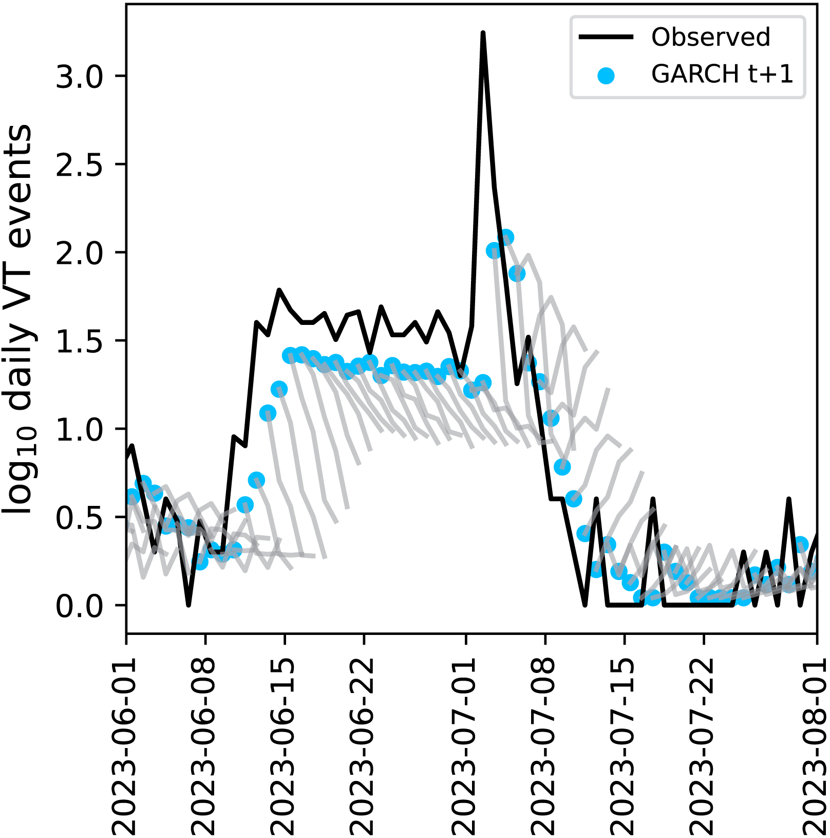
4.3. Comparison with previous studies
Our results align with previous work showing that volcanic time series are inherently difficult to forecast, but they also reveal important differences in which factors enable or constrain predictability. A comprehensive review by Whitehead and Bebbington (2021) highlighted that no single forecasting method consistently outperforms others across different volcanic systems, emphasizing the importance of system-specific characteristics in determining forecast skill.
Several studies have explored time series forecasting at various volcanoes, with varying degrees of success. At Soufrière Hills volcano, Hammer and Ohrnberger (2012) used dynamical models of earthquake rates to forecast the number of seismo-volcanic events, achieving interesting results during periods of dome growth. At Whakaari (White Island), New Zealand, Dempsey, Cronin, et al. (2020) developed automated precursor recognition systems using decision trees on Real-time Seismic-Amplitude Measurement (RSAM) data, successfully identifying short-term precursors to phreatic eruptions. More recently, Ardid et al. (2025) also leveraged RSAM and other seismic amplitude features from multiple volcanic systems to implement ML models able to provide short-term eruption forecasts. Zali et al. (2024) used clustering to reveal pre-eruptive tremor signals at the 2021 Geldingadalir eruption in Iceland, demonstrating that sophisticated pattern recognition can extract meaningful precursors even from complex datasets. Chastin and Main (2003) demonstrated that daily seismic event rate data could serve as eruptive precursors at Kilauea when analyzed with appropriate statistical frameworks, but only at short term. The study of Manley et al. (2021) of the 2006 Augustine volcano eruption suggests that integrating multiple types of data may help to forecast unrest and eruptions via ML novelty detection or supervised classification. Finally, another interesting study in the present context is that of Luongo et al. (2004). This study evaluated the ability of artificial neural networks to forecast either seismicity or deformation at Etna, Phlegrean Fields, Vesuvius and Kilauea, using time series recorded at different rates. We are particularly interested in their attempt to forecast the monthly seismicity at Vesuvius between April 1972 to July 2000. They obtained a R2 of 0.72 for t + 1 month test predictions (December 1998–July 2000). This value is better than ours of 0.62 obtained with the model from Section 3.1 at the t + 1 day horizon. However, their data consist of monthly observations during a quiescent period (peaking at less than 180 events/month) and thus are much less volatile, making them inherently easier to forecast.
From the results of those studies and the present one, we identified several key factors that affect forecasting performance:
Signal regularity
Processes characterized by quasi-periodic behavior with consistent timing and amplitude, such as caldera collapses during a same sequence (McBrearty and Segall, 2024), yield signals easier to forecast than variable and volatile signals generated by statistically rare events, such as Piton de la Fournaise eruptions.
Available pre-eruptive signalsDuring unrest, daily VT counts and GNSS baseline gradients at Piton de la Fournaise show subtle changes compared to background variability. Studies have shown that for some other volcanic systems, pre-eruptive tremor can be extracted and largely benefit unrest detection (Zali et al., 2024). However, at Piton de la Fournaise such signals have not been observed and the tremor appears when the eruption starts, i.e. when there is lava flow at surface.
Data type and resolutionSome successful studies used continuous waveform-derived features (RSAM, containing tremor energy) rather than discrete event counts. These features may better capture evolving volcanic processes, and be more stable for machine learning applications.
Forecast objectiveBinary classification of eruptive state (eruption versus no eruption) or event detection (identifying when a collapse will occur or an abnormal signal) may be more tractable than continuous multi-day forecasting of time series values.
4.4. Paths forward for volcanic time series forecasting
The above observations suggest that predictability in volcanic forecasting is strongly controlled by the characteristics of the volcanic system, the nature of available observables, and the specific forecasting task, rather than solely by the choice of algorithm. Volcanoes exhibiting more periodic or cyclical behavior, higher signal-to-noise ratios, or more comprehensive monitoring networks offer better prospects for successful forecasting, regardless of whether simple or complex models are employed. For systems such as Piton de la Fournaise with irregular eruptive precursor patterns, alternative approaches focusing on anomaly detection, probabilistic forecasting, or binary state classification may prove more operationally useful than continuous time series forecasting. Given the data limitations identified, several other strategies could improve forecasting performance at Piton de la Fournaise, and possibly at similar volcanic systems.
First, enhanced data selection, feature engineering, and data fusion seem necessary. For instance, including earthquake magnitudes and type, spatial distributions (e.g., centroid locations, spatial clustering metrics), and energy release characteristics would provide models with information about the spatial and energetic evolution of the seismic process linked to magma propagation. Similarly, incorporating deformation source inversions (e.g., model parameters tracking source depth and volume changes) and any other physics-informed features derived from physical models of volcanic processes could also enhance predictability. In addition, geochemical data such as CO2 and SO2 emissions near the volcano summit could also be added.
Second, synthetic data generation techniques could be explored to address the limited number of eruptive examples. For instance, physics-based simulations of magma transport and storage (Segall, 2013), combined with realistic noise models, could generate diverse pre-eruptive scenarios. Generative machine learning models (e.g. generative adversarial networks) trained on existing data could also produce synthetic precursory patterns. This will require (i) the validation of any synthetic data to ensure that it captures realistic volcanic behavior and (ii) the implementation of rigorous tests of models trained on synthetic data against real observations.
Third, several ML methodological directions could be pursued. If physics-based models are available, hybrid physics-ML approaches could leverage both physical understanding and data-driven pattern recognition. For example, physics-based models could constrain the space of possible seismicity or deformation evolution, and this could be provided as input to the ML models. Transfer learning, which implies pre-training models on data from multiple volcanic systems and then using them to make predictions on a new volcano with or without additional fine-tuning, may also help address the limited eruptive examples at any single volcano. This approach appears promising, as shown by the recent studies of Ardid et al. (2025) and Zhong and Tan (2024). Transfer learning approaches could leverage patterns common across systems while adapting to local characteristics. However, this requires careful consideration of similarities and differences in volcanic behavior, monitoring network geometry, and data quality between sites.
However, even if the data and model limitations are solved, other challenges remain. For instance, for operational purposes, forecasting models must provide reliable uncertainty estimates to inform decision-making. Deterministic forecasts, as explored in this study, provide limited operational value when uncertainty is high. Future approaches should explicitly represent forecast uncertainty. Gaussian processes (Roberts et al., 2013), Bayesian neural networks, or ensemble methods could provide probabilistic forecasts with confidence intervals. Such approaches would be more consistent with operational volcanic hazard assessment frameworks that increasingly emphasize probabilistic formulations (Marzocchi et al., 2008; Dempsey, Kempa-Liehr, et al., 2022; Christophersen et al., 2022).
To conclude, we emphasize that even with current limitations, forecasting models could complement existing threshold-based alarm systems at volcano observatories. At Piton de la Fournaise, operational thresholds are based on observed seismicity (Peltier, Villeneuve, et al., 2018; Peltier, Ferrazzini, Di Muro, et al., 2021). Short-term forecasts of seismic or deformation trends, even if imperfect, could provide early warnings of anomalous behavior before thresholds are crossed. Forecast of GNSS signal source could help refine anticipated locations of dike propagation. Combined with seismic forecasts in multiparametric alarm systems, this could enable earlier and more reliable detection of magma injections.
5. Conclusion
This study evaluated the potential of machine learning approaches to forecast the data used operationally by OVPF-IPGP to monitor Piton de la Fournaise: the daily number of VT events and the daily GNSS deformation data. Results show the inherent difficulty of predicting such highly stochastic datasets. No single method consistently outperformed the others. Transformer models proved quite effective for seismicity, while Linear models performed best for deformation data. Combining seismicity and deformation datasets was not key to achieving better results. Econometric methods such as GARCH showed no advantage in handling volatility, and, like ML models, failed to anticipate sharp pre-eruptive changes.
These findings highlight the challenges of forecasting low-signal, non-periodic volatile volcanic time series. With the data we used, only first-order trends can be reliably forecast; abrupt changes linked to the sudden evolution of volcanic system activity are difficult to predict. These results are a first step toward bridging data-driven forecasts with operational volcano monitoring at Piton de la Fournaise. They allow identifying several avenues to improve forecasting signals at Piton de la Fournaise and possibly other volcanoes, such as adding new data types and features, generating synthetic data, and leveraging hybrid methods, transfer learning, and probabilistic forecasting.
Acknowledgments
The seismic and GNSS data presented in this paper were collected by Observatoire Volcanologique du Piton de la Fournaise, Institut de Physique du Globe de Paris (OVPF-IPGP, doi: 10.18715/REUNION.OVPF). We thank the Service National d’Observation en Volcanologie (SNOV-CNRS-INSU) for the use of data. The correction of English in the manuscript benefited from assistance provided by generative AI large language models.
Declaration of Interests
The authors do not work for, advise, own shares in, or receive funds from any organization that could benefit from this article, and have declared no affiliations other than their research organizations.
Funding
This work was supported by funding from the Data Intelligence Institute of Paris (diiP), IdEx Université Paris Cité (ANR-18-IDEX-0001), to MN, and an ANR INSU TelluS-SYSTER grant to CLL, LR and AP.
Supplementary materials
The data and computer code for reproducing this study are available on Zenodo (Nougaret and Le Losq, 2025).