Impact of integration time steps of rain drop size distribution on their structuring and their modelling: a case study in northern Benin

Sounmaïla Moumouni; Loïc Saturnin Adjikpé; Agnidé Emmanuel Lawin

doi:10.5802/crgeos.55

Article original - Géophysique externe, Climat

Impact of integration time steps of rain drop size distribution on their structuring and their modelling: a case study in northern Benin

Sounmaïla Moumouni ¹ ; Loïc Saturnin Adjikpé ² ; Agnidé Emmanuel Lawin ³

¹ Higher Teachers’ Training School of Natitingou, National University of Sciences, Technologies, Engineering and Mathematics, Benin
² Department of Physics, Faculty of Science and Technology, University of Abomey-Calavi, Benin
³ Laboratory of Applied Hydrology (LHA), National Water Institute (INE), 01 BP: 4521 Cotonou, Benin

Comptes Rendus. Géoscience, Volume 353 (2021) no. 1, pp. 135-153.

Résumé

This paper focused on modelling rain drop size distributions (DSDs) of various integration time steps using unimodal DSD models (gamma and lognormal). Rain DSD data considered are those collected from 2005 to 2007 near Djougou city in the north-western region of Benin Republic. The efficiency of these models was characterized by statistical criteria, mainly Nash and KGE. These criteria are used to assess the level of fitting of rain DSD spectra. Superimposed rain DSDs were then parameterized with the rainfall rate, using the scaling law formalism. Results show that there is an improvement in the structuring of the rain DSDs according to their measurement duration. Analysis of the occurrence statistics of the structuring of the spectra reveals that the Spectra ill adjusted by a unimodal DSD model represents 5 to 15% of the population of 1 min rain DSDs. This population decreases according to the measurement duration of the spectra. The optimal measurement time is found to be 10 min. Furthermore, parameters of the shape functions (gamma and lognormal) increase or decrease markedly according to the measurement duration of the rain DSD spectra. For applications using the relationships deduced from the rain DSDs, results suggested that the measurement time scale must be taken into account when choosing appropriate relationships.

Métadonnées

Reçu le : 2020-07-04
Révisé le : 2021-02-04
Accepté le : 2021-04-19
Publié le : 2021-05-27

DOI : 10.5802/crgeos.55

Mots clés : Rain DSD, Scaling law, Unimodal DSD models, Rainfall, Parameterization, Integration time steps, West Africa

Affiliations des auteurs :

Sounmaïla Moumouni ¹ ; Loïc Saturnin Adjikpé ² ; Agnidé Emmanuel Lawin ³

Licence :

CC-BY 4.0

Droits d'auteur : Les auteurs conservent leurs droits

@article{CRGEOS_2021__353_1_135_0,
     author = {Sounma{\"\i}la Moumouni and Lo{\"\i}c Saturnin Adjikp\'e and Agnid\'e Emmanuel Lawin},
     title = {Impact of integration time steps of rain drop size distribution on their structuring and their modelling: a case study in northern {Benin}},
     journal = {Comptes Rendus. G\'eoscience},
     pages = {135--153},
     publisher = {Acad\'emie des sciences, Paris},
     volume = {353},
     number = {1},
     year = {2021},
     doi = {10.5802/crgeos.55},
     language = {en},
}

TY  - JOUR
AU  - Sounmaïla Moumouni
AU  - Loïc Saturnin Adjikpé
AU  - Agnidé Emmanuel Lawin
TI  - Impact of integration time steps of rain drop size distribution on their structuring and their modelling: a case study in northern Benin
JO  - Comptes Rendus. Géoscience
PY  - 2021
SP  - 135
EP  - 153
VL  - 353
IS  - 1
PB  - Académie des sciences, Paris
DO  - 10.5802/crgeos.55
LA  - en
ID  - CRGEOS_2021__353_1_135_0
ER  -

%0 Journal Article
%A Sounmaïla Moumouni
%A Loïc Saturnin Adjikpé
%A Agnidé Emmanuel Lawin
%T Impact of integration time steps of rain drop size distribution on their structuring and their modelling: a case study in northern Benin
%J Comptes Rendus. Géoscience
%D 2021
%P 135-153
%V 353
%N 1
%I Académie des sciences, Paris
%R 10.5802/crgeos.55
%G en
%F CRGEOS_2021__353_1_135_0

Sounmaïla Moumouni; Loïc Saturnin Adjikpé; Agnidé Emmanuel Lawin. Impact of integration time steps of rain drop size distribution on their structuring and their modelling: a case study in northern Benin. Comptes Rendus. Géoscience, Volume 353 (2021) no. 1, pp. 135-153. doi : 10.5802/crgeos.55. https://comptes-rendus.academie-sciences.fr/geoscience/articles/10.5802/crgeos.55/

Version originale du texte intégral (Proposez une traduction )

1. Introduction

Several studies are carried out on the spectra of the rain drop size distributions (DSDs), which are not well-fitted by unimodal DSD models, in particular, those which have several peaks (multimodal spectra) [Ekerete et al. 2015a,b, 2016; Radhakrisna and Narayana Rao 2009; Sauvageot and Koffi 2000]. To identify the peaks in the rain DSDs, measured on the ground, Steiner and Waldvogel [1987] used the following principle: if the concentration N(D) of a given diameter is significantly higher than those of neighbouring diameters, then a peak exists at this diameter. Radhakrisna and Narayana Rao [2009] and Sauvageot and Koffi [2000] simplified this principle as follows: a diameter D_i (i is the index of a diameter class in a rain DSD spectrum) has a peak if only N(D_i−1) < N(D_i) > N(D_i+1). Radhakrisna and Narayana Rao [2009] applied this method and obtained around 30% of multimodal spectra in their rain DSDs data, with integration time T = 5 min, observed on the ground, at Gadanki in India. Ekerete et al. [2015b], Ekerete et al. [2015a] and Ekerete et al. [2016] suggested that this method is not sufficient to properly identify multimodal spectra. A multimodal spectrum being made up of several sub-spectra separated by hollow, each sub-spectrum having a peak (or a mode), they propose to identify the number of peaks from the number of hollow. Thus, a diameter D_i has a hollow if only N(D_i−1) > N(D_i) < N(D_i+1) < N(D_i+2). Before applying this method, Ekerete et al. [2015b], Ekerete et al. [2015a] and Ekerete et al. [2016] merged into a spectrum, five neighbouring spectra of 1 min duration, to smooth the data. With the disdrometric data from Chilbolton in England, Ekerete et al. [2015b] obtained 51% of multimodal spectra. In contrast with the disdrometric data from Graz in Austria, Ekerete et al. [2016] obtained around 28% of multimodal spectra, a proportion similar to that of Radhakrisna and Narayana Rao [2009].

Sauvageot and Koffi [2000] indicated that the rain DSDs observed over a short period generally has an erratic shape, with several relative maximums. They found these multimodal shapes in the disdrometric data acquired in two climatic regions: one tropical (Boyélé in Congo), and the other temperate (Brest in France). They also showed that some modes of rain DSDs have a persistence larger than several minutes. They then suggested that the analysis of the rain DSDs observed on the ground are superimposed DSDs.

Radhakrisna and Narayana Rao [2009] attempted for the first time to answer several key questions concerning the multimodality of rain DSDs, using data collected in Gadanki, India. The author assessed the occurrence statistics and their dependency on height, season, and type of precipitation. Among other things, they noted that multimodal shapes are not only observed on the ground. They are rather observed at all altitudes, but with different percentages of occurrence.

Recently, Ekerete et al. [2015b] have shown, from data acquired in the south of England, that multimodality of rain DSDs is a relatively common phenomenon. Analysing this multimodality of rain DSD, Ekerete et al. [2015a] fit these multimodal spectra with a Gaussian mixture model. Ekerete et al. [2016] showed that the average number of modes tends to increase depending on wind speed and rain rate.

Therefore, some rain DSD spectra, whether observed on the ground or at altitude, can be multimodal. This does not allow unimodal DSD models (such as gamma or lognormal) to adjust them individually, suitably. The efficiency of individual modelling of rain DSD spectra, with unimodal DSD models, can be assessed using statistical criteria such as Nash or KGE (see Appendix). Thus, a rain DSD spectrum can be ill or well adjusted by a unimodal model for certain values of these criteria. Multimodal spectra will naturally be ill adjusted by a unimodal model.

Furthermore, from rain DSDs data with duration T = 1 min, it is possible to create DSD datasets with integration time steps T = L min (where L is a natural integer greater than one) by calculating the averages of the L successive spectra, as [Chapon et al. 2008] did. A temporal filtering of the rain DSDs is thus carried out, making it possible to build up datasets of various integration time steps. We can also individually adjust these new spectra by unimodal model and assess their level of structuring. This is why one of the objectives of this article focused on investigating the impact of the integration time steps of rain DSDs on their structure. Specifically, we analysed the impact of the integration time step of the rain DSDs: (1) on the structuring of the rain DSD spectra; and (2) on the parameterization of rain DSDs by the rain rate.

Data	DATA1	DATA2	DATA3	DATA4	DATA5	DATA6
Integration time steps	T = 1 min	T = 2 min	T = 5 min	T = 10 min	T = 15 min	T = 20 min
Number of spectra	12,342	6152	2437	1198	777	578
Cumulative (mm)	1237.16	1236.89	1235.53	1225.94	1217.20	1216.79

Thus, in Sections 2, 3, and 4, we respectively presented the datasets, the methodology used, and the results and their analysis. Finally, Sections 5 and 6 respectively represent the discussion and the concluding remarks.

2. Datasets

The DSDs data used for this study are those sampled in northern Benin, near the town of Djougou (9.66° N, 1.69° E)—using optical disdrometers: single beam [Löffler-Mang and Joss 2000; Salles 1995; Salles et al. 1998] and double beam [Delahaye et al. 2005]—from 2005 to 2007, during the African Monsoon Multidisciplinary Analysis (AMMA) meteorological campaign. These data have been validated and widely used for several studies [Gosset et al. 2010; Kougbéagbédè et al. 2017; Moumouni 2009; Moumouni et al. 2008, 2018]. These data are DSDs of rains with an integration time step equal to 1 min. They are made up of 93 rainy events which represent a total of: 11,647 spectra when only rain intensities greater than or equal to 0.1 mm⋅h⁻¹ are taken into account; and 12,342 spectra when only rainfall intensities greater than or equal to 0.05 mm⋅h⁻¹ are taken into account. The selected rainy events are isolated at the level of each disdrometer. A rainy event is defined as event with duration at least equal to 15 min and intermittency less than 30 min.

From these data, other rain DSDs datasets of various integration time steps were computed (Table 1). The DSDs duration T = L min were calculated within each event, and the remaining spectra whose number is less than L are not taken into account.

3. Methods

Since the pioneering work of Marshall and Palmer [1948] on the rain DSDs, most of those which followed, such as [Atlas et al. 1999; Cerro et al. 1997; Chen et al. 2019; Tenorio et al. 2012; Tokay and Short 1996; Uijlenhoet et al. 2003; Ulbrich 1983; Ulbrich and Atlas 1998; Wen et al. 2018; Willis 1984; Zeng et al. 2019; Zhang et al. 2003; etc.], analyse it with N(D) function, defined by spectrum of a given period T (1 min). It corresponds to the number of raindrops per unit of volume and by interval of diameters and is calculated as follows:

\begin{matrix} N (D_{i}) = \frac{N_{i}}{S T 𝛥 D_{i} V (D_{i})}, \end{matrix}

(1)

where

D_{i}

is the equivalent diameter of the raindrops measured, 𝛥D_i the width of the range of diameter centred on D_i. In this study, D_i and 𝛥D_i are expressed in millimetres. S is the disdrometer collecting surface area expressed in square metre. At the period T, N_i is the number of drops counted by the disdrometer in each size range. V (D_i) is the falling speed of the drops of diameter D_i. For the rain rate to be proportional to a moment of N(D) function, the relationship between the drops speed and their diameter is used as suggested by Atlas and Ulbrich [1977]

V (D_{i}) = 3.78 D_{i}^{0.67} (m \cdot s^{- 1})

(2)

In all the above studies,

T = 1 min = 60 s

and N(D_i) is expressed in (m⁻³⋅mm⁻¹).

3.1. The structuring of the measured spectra

In West Africa where our data were collected, all the studies [Gosset et al. 2010; Kougbéagbédè et al. 2017; Moumouni et al. 2008; Moumouni 2009; Moumouni et al. 2018; Nzeukou et al. 2004; Ochou et al. 2007; Sauvageot and Lacaux 1995] showed that the superimposed rain DSDs can be well adjusted by the gamma DSD model or the lognormal DSD model. In this study, we then used these two models to individually fit the rain DSD spectra. After fitting a DSD model (gamma or lognormal) on a measured spectrum, Nash and KGE criteria are calculated (see Appendix) between the measured spectrum and the modelled spectrum. The values of these criteria are therefore indicators of the efficiency of the modelling. If the measured spectrum is well adjusted by a unimodal DSD model, the criteria will indicate a good level of efficiency. If, on the other hand, the spectrum is not well adjusted by a unimodal DSD model, the criteria will indicate a low level of efficiency. These criteria are therefore used to qualify the state of structuring of the measured spectrum. These structuring levels of the spectra are analysed according to the integration time steps of the rain DSDs.

The measured moment of order n of a rain DSD spectrum (whatever the integration time steps) is defined [Chapon et al. 2008; Lee et al. 2004; Ochou et al. 2007; Sempere-Torres et al. 1994; Zeng et al. 2019] by

M_{n} = \sum_{i} D_{i}^{n} N (D_{i}) 𝛥 D_{i}

(3)

When we assume a DSD model, the theoretical moment of order $n$ of a rain DSD spectrum (whatever the integration time steps) is defined [Chapon et al. 2008; Lee et al. 2004; Ochou et al. 2007; Sempere-Torres et al. 1994; Zeng et al. 2019] by

M_{n} = \int_{0}^{+ \infty} D^{n} N (D) d D

(4)

3.1.1. Gamma DSD model fitting

In the literature on rain DSD, there are several variants of writing the gamma DSD model. For example, the form proposed by Ulbrich [1983] and Maki et al. [2001] is different from that proposed by Testud et al. [2001] or Lee et al. [2004]. In this study, we propose the following form to have a model whose parameters have well-known physical meanings

N (D) = \frac{N_{T} {(𝜇 + 1)}^{(𝜇 + 1)}}{D_{a} 𝛤 (𝜇 + 1)} {(\frac{D}{D_{a}})}^{𝜇} exp [- (𝜇 + 1) \frac{D}{D_{a}}]

(5)

Indeed, in a spectrum, $N_{T}$ is the total number of drops per unit of volume, D_a is the arithmetic mean of diameter of the drops, and 𝜇 is the shape parameter of the spectrum. By introducing the expression (5) in (4), the moment of order n is

\begin{matrix} M_{n} = \frac{N_{T}}{𝛤 (𝜇 + 1)} {(\frac{D_{a}}{𝜇 + 1})}^{n} 𝛤 (𝜇 + n + 1) \end{matrix}

(6)

For fitting this model on the measured spectra, with the moments method, its parameters $N_{T} (m^{- 3})$ , D_a (mm), and 𝜇, can be estimated, from the measured moments, with the following formulae

\begin{matrix} N_{T} = M_{0}, D_{a} = \frac{M_{1}}{M_{0}}, 𝜇 = \frac{M_{0} M_{2} - 2 M_{1}^{2}}{M_{1}^{2} - M_{0} M_{2}} \end{matrix}

(7)

3.1.2. Lognormal DSD model fitting

Lognormal model with three parameters used to describe the rain DSD is proposed by Feingold and Levin [1986]

\begin{matrix} N (D) = \frac{N_{T}}{\sqrt{2 π} D ln 𝜎} exp [- \frac{{ln}^{2} (D ∕ D_{g})}{2 {ln}^{2} 𝜎}] \end{matrix}

(8)

In this expression,

N_{T}

is the total number of drops per unit of volume, D_g is the geometric mean of diameter of the drops, 𝜎 is the shape parameter of the spectrum. By introducing the expression (8) in (4), the moment of order n is

\begin{matrix} M_{n} = N_{T} D_{g}^{n} exp (\frac{1}{2} n^{2} {ln}^{2} 𝜎) \end{matrix}

(9)

For fitting this model on the measured spectra, with the moments method, its parameters

N_{T} (m^{- 3})

, D_g (mm), and 𝜎, can be estimated, from the measured moments, with the following formulae

\begin{matrix} \begin{matrix} N_{T} = M_{0}, D_{g} = \frac{M_{1}}{M_{0}} \sqrt{\frac{M_{1}^{2}}{M_{0} M_{2}}}, \\ 𝜎 = exp [\sqrt{- ln (\frac{M_{1}^{2}}{M_{0} M_{2}})}] \end{matrix} \end{matrix}

(10)

3.2. Parameterization of drop size distribution with rain rate

There are two methods of parameterizing of the rain DSDs by the rain rate: the method based on the calculation of the average spectra by rain rate class [Nzeukou et al. 2004; Ochou et al. 2007; Sauvageot and Lacaux 1995] and the scaling law method [Chapon et al. 2008; Sempere-Torres et al. 1994; Sempere Torres et al. 1998]. In this study, we preferred the second method because it offers well-defined scale parameters that can be easily analysed according to the integration time steps of DSDs.

3.2.1. Summary of the scaling law formalism

Proposed by Sempere-Torres et al. [1994], the parameterization of the DSDs by the rain rate $R$ , is written as follows:

\begin{matrix} N (D) = R^{𝛼} g (D R^{- 𝛽}) \end{matrix}

(11)

In this expression,

g

is a shape function which should model the DSDs regardless of the scaling parameter (R). The constants 𝛼 and 𝛽 are determined by assuming a power relationship between the moments of the DSD and the rain rate

\begin{matrix} M_{n} = A_{n} R^{b_{n}} \end{matrix}

(12)

By carrying expression (11) in formula (4) and making the change of variable (

x = D R^{- 𝛽}

), we obtain

\begin{matrix} M_{n} = [\int_{0}^{+ \infty} x^{n} g (x) d x] R^{𝛼 + (n + 1) 𝛽} \end{matrix}

(13)

Thus, by comparing (12) and (13) we have

b_{n} = 𝛼 + (n + 1) 𝛽

(14)

and

A_{n} = \int_{0}^{+ \infty} x^{n} g (x) d x

(15)

Moreover, the rain rate is defined [Chapon et al. 2008; Sempere Torres et al. 1998] by

\begin{matrix} R = C_{R} M_{3.67} with C_{R} = \frac{22.68 π}{1 0^{4}} \end{matrix}

(16)

By comparing (16) and (13) we deduce the following relationships

𝛼 + 4.67 𝛽 = 1

(17)

and

C_{R} \int_{0}^{+ \infty} x^{3.67} g (x) d x = 1

(18)

The relation (17) creates a constraint between the constants

𝛼

and 𝛽, while the integral equation (18) is used to reduce the number of parameters of the shape function.

3.2.2. Shape function with the gamma DSD model

When we assume that the rain DSDs are gamma-shaped, Chapon et al. [2008] proposed the following expression for the shape function

\begin{matrix} g (x; 𝜅, 𝜇, 𝜆) = 𝜅 x^{𝜇} exp (- 𝜆 x) \end{matrix}

(19)

By introducing the expression (19) in (18), we obtain the following equation which makes it possible to reduce to two the number of parameters of the shape function

\begin{matrix} 𝜅 = 𝜆^{(𝜇 + 4.67)} {[C_{R} 𝛤 (𝜇 + 4.67)]}^{- 1} \end{matrix}

(20)

When we introduce (20) in (19), the shape function of the gamma DSD model becomes

\begin{matrix} g (x; 𝜇, 𝜆) = 𝜆^{(𝜇 + 4.67)} {[C_{R} 𝛤 (𝜇 + 4.67)]}^{- 1} x^{𝜇} exp (- 𝜆 x) \end{matrix}

(21)

The estimation of the shape function

g

therefore boils down to the estimation of two parameters 𝜇 and 𝜆. Furthermore, when we carry the expression (21) of the shape function in formula (15), we obtain

\begin{matrix} A_{n} = \frac{𝜆^{(3.67 - n)} 𝛤 (𝜇 + n + 1)}{C_{R} 𝛤 (𝜇 + 4.67)} \end{matrix}

(22)

Categories	Spectra very well adjusted by a unimodal DSD model	Spectra well adjusted by a unimodal DSD model	Spectra ill adjusted by a unimodal DSD model
Criterion 1	$Nash ⩾ 0.8$	0.6⩽Nash < 0.8	Nash < 0.6
Criterion 2	KGE⩾0.8	0.6⩽KGE < 0.8	KGE < 0.6

3.2.3. Shape function with the lognormal DSD model

Assuming that the rain DSDs are lognormal-shaped, in the same approach as [Chapon et al. 2008], we propose the following expression for the shape function

\begin{matrix} g (x; 𝜒, 𝜎, 𝜃) = \frac{𝜒}{\sqrt{2 π} x ln 𝜎} exp [- \frac{{ln}^{2} (x ∕ 𝜃)}{2 {ln}^{2} 𝜎}] \end{matrix}

(23)

By introducing the expression (23) in (18), we obtain the following equation which makes it possible to reduce to two the number of parameters of the shape function

\begin{matrix} 𝜒 = C_{R}^{- 1} 𝜃^{- 3.67} exp [- 0.5 (3.6 7^{2}) {ln}^{2} 𝜎] \end{matrix}

(24)

When we introduce (24) in (23), the shape function of the lognormal DSD model becomes

g (x; 𝜎, 𝜃) = \frac{exp (- 0.5 (3.6 7^{2}) {ln}^{2} 𝜎)}{C_{R} 𝜃^{3.67} \sqrt{2 π} x ln 𝜎} exp [- \frac{{ln}^{2} (x ∕ 𝜃)}{2 {ln}^{2} 𝜎}]

(25)

The estimation of the shape function $g$ therefore boils down to the estimation of two parameters 𝜎 and 𝜃. Furthermore, when we carry the expression (25) of the shape function in formula (15), we obtain

\begin{matrix} A_{n} = \frac{exp [0.5 (n^{2} - 3.6 7^{2}) {ln}^{2} 𝜎]}{C_{R} 𝜃^{(3.67 - n)}} \end{matrix}

(26)

3.2.4. Implementation of the scaling law formalism

In this article, for each integration time step of the rain DSDs, the scaling law approach will be executed successively as follows:

Calculation of moments of order $n$ (M_n) and of the rain rate (R) from the data of measured rain DSDs.
Determination of the exponents b_n and of the pre-factor A_n in an empirical way (linear regression of (12)).
Estimation of the constants 𝛼 and 𝛽, from the values of b_n. This estimation is done empirically (linear regression of (14)).
Estimation of the shape functions: Chapon et al. [2008] used the method of moments combined with (18). The approach used in this article, for each model, is described as follows:
- For the shape function of the gamma DSD model, it is necessary to estimate the values of the parameters 𝜇 and 𝜆. We did a regression in the least squares sense of (22) compared to the values of A_n obtained in step no. 2.
- For the shape function of the lognormal DSD model, it is necessary to estimate the values of the parameters 𝜎 and 𝜃. We made a regression in the least squares sense of (26) compared with the values of A_n obtained in step no. 2.
Calculation of the normalized spectra with (11), then representation of these spectra and the shape functions (gamma and lognormal).
Validation of the modelling: use of different statistical criteria to compare the theoretical moments (12) with the measured moments (3). In expression (12), the exponent is calculated with (14), the pre-factor for the gamma distribution is determined with (22), and the pre-factor for the lognormal distribution is determined with (26).

4. Results

4.1. Structuring of rain DSDs spectra

Figure 1 is an example of 1 min rain DSD spectra. These are all multimodal spectra. The values of the displayed efficiency criterion indicate that these spectra cannot be adjusted by unimodal DSD models. To each model adjusting the rain DSD measured is assigned two criteria. We have created three categories of spectra based on their level of adjusting, as shown in Table 2. To assess the percentage of occurrence of the level of structuring of these spectra, we have presented in Figure 2 the percentiles of each criterion. With the 1 min rain DSDs, depending on the criteria and models, we noted that: 5 to 15% of the spectra are ill adjusted by a unimodal DSD model; and about 60% of the spectra are very well adjusted by a unimodal DSD model. The number of ill-adjusted and well-adjusted spectra decreases in favour of very well-adjusted spectra, as the integration time steps increases. This is also confirmed in Figure 3. We noted that from T = 10 min, the proportion of the three spectral types is almost stable. Figure 4 also illustrates the effect of the integration time steps of the DSDs on their structuring. The unframed spectra (top and bottom) are 1 min spectra. The majority of the top spectra are not well adjusted by the unimodal DSD models. But, their resultant (5 min spectrum) is very well adjusted by the unimodal DSD models. Moreover, the majority of the lower spectra are very well adjusted by the unimodal DSD models. Their resultant (5 min spectrum) is also very well adjusted by the unimodal DSD models. Finally, we notice that the resultant of the ten spectra (bottom and top) is better adjusted than each of the 5 min spectra.

Figure 1.
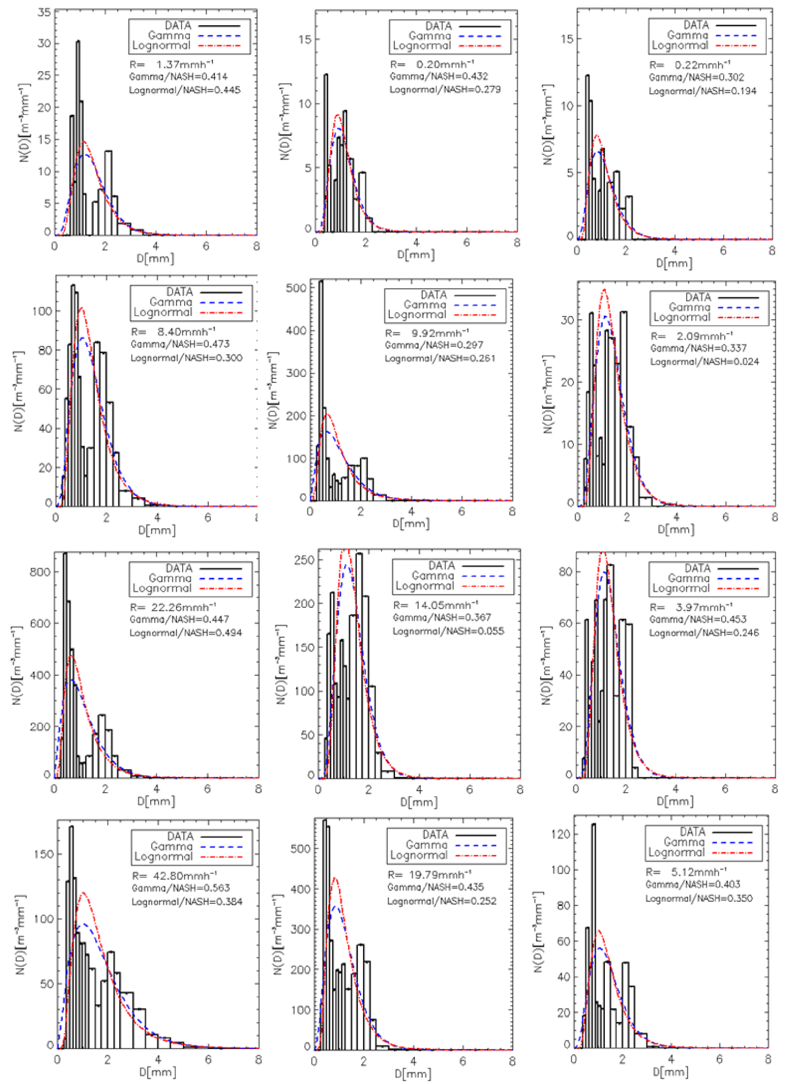
Some measured 1 min rain DSD spectra, their rainfalls rate, and the values of the Nash efficiency criterion (relating to gamma DSD model and lognormal DSD model).

Figure 2.
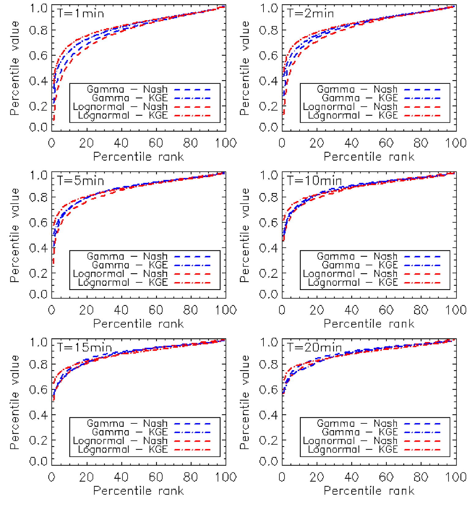
The percentiles of the efficiency criteria (Nash and KGE) relating to the gamma and lognormal DSD models fitting measured spectra (for each integration time steps).

Figure 3.
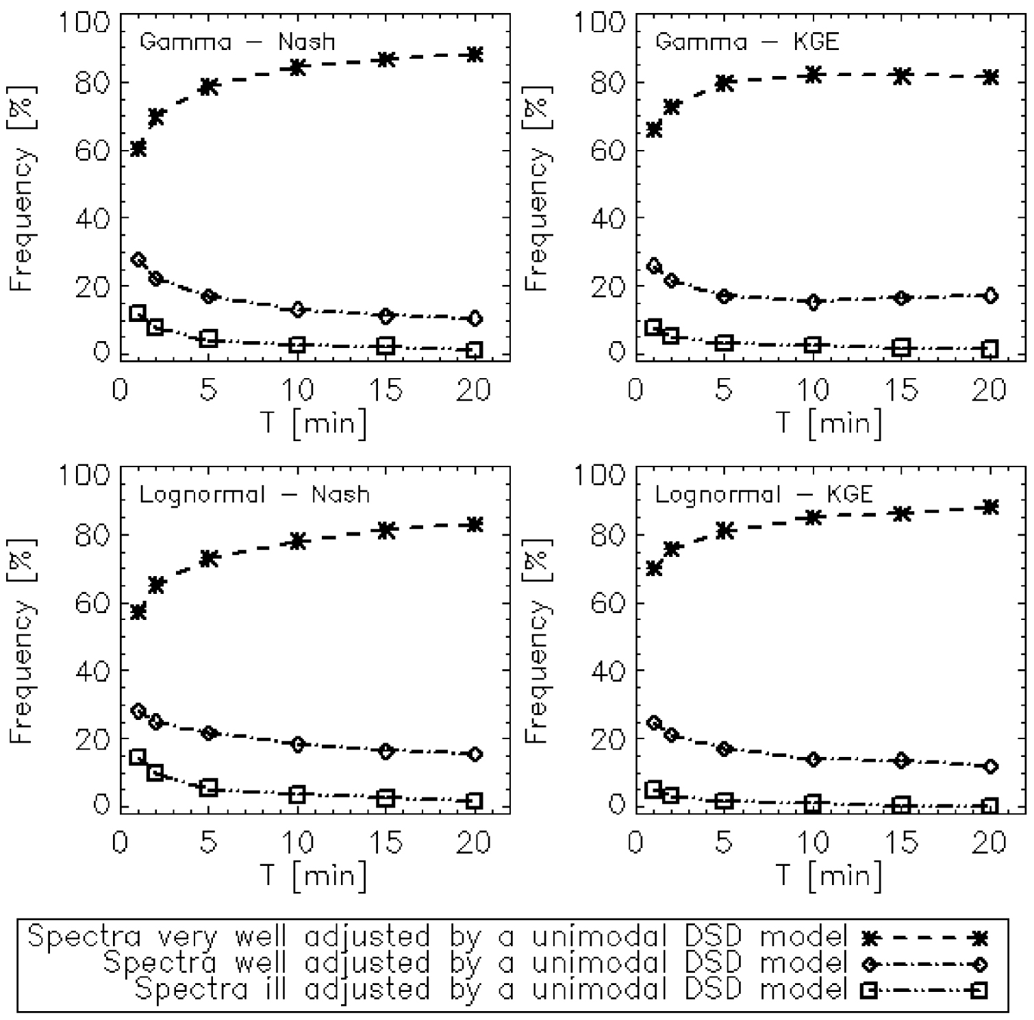
Frequency of the three categories of spectra (taking into account the efficiency of their adjustment) as a function of the integration time steps of the rain DSDs.

Figure 4.
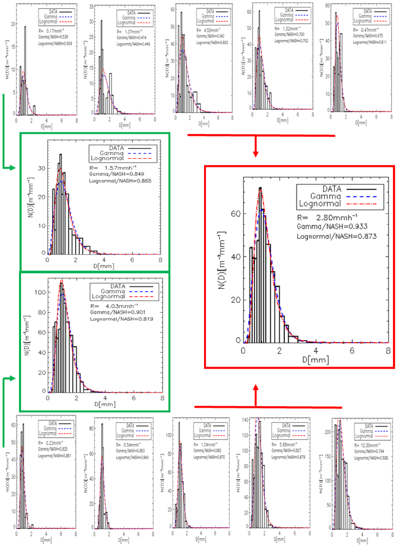
Illustration of the effect of the integration time steps of the DSDs on their structuring. The unframed spectra (top and bottom) are 1 min spectra. Spectra framed in green are 5 min spectra. The spectrum framed in red is a 10 min spectrum.

The temporal filtering of DSDs therefore makes it possible to significantly reduce the number of spectra that cannot be adjusted by unimodal DSD models. Then, T = 10 min is the optimal duration of measurement for a good structuring of all the spectra of the dataset.

4.2. Parameterization of rain DSDs by rainfall rate

Table 3 presents the values of the exponents b_n and of the pre-factor A_n. Figure 5 describes the estimation of the constants 𝛼 and 𝛽, for the six integration time steps chosen. These constants, listed in Table 4, are all positive, whatever T. Thus, confirming that the rain rate increases as a function of the number of drops and the size of the drops.

Figure 5.
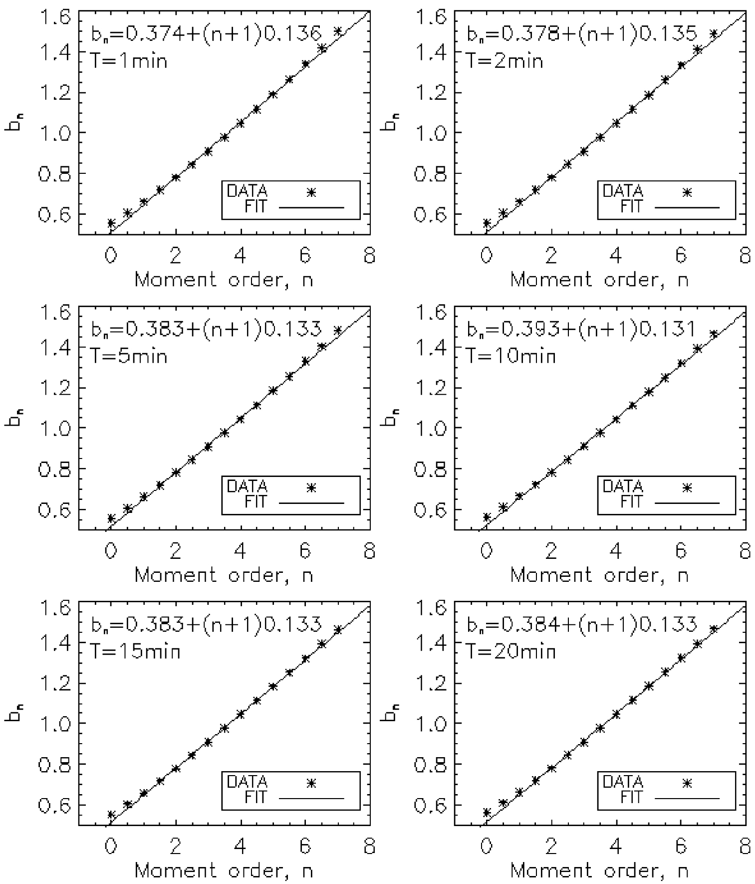
Estimating of the constants 𝛼 and 𝛽: the exponent b_n (relation (14)) according to the order of the moments (Table 3), for each integration time steps.

n	T = 1 min		T = 2 min		T = 5 min		T = 10 min		T = 15 min		T = 20 min
	b_n	A_n	b_n	A_n	b_n	A_n	b_n	A_n	b_n	A_n	b_n	A_n
0.0	0.557	71.28	0.556	71.28	0.558	70.66	0.565	69.71	0.553	70.22	0.561	68.88
0.5	0.607	70.84	0.606	70.72	0.609	70.00	0.614	69.00	0.604	69.29	0.610	68.12
1.0	0.661	72.85	0.661	72.62	0.663	71.82	0.667	70.77	0.659	70.89	0.663	69.87
1.5	0.719	77.38	0.719	77.07	0.721	76.22	0.724	75.13	0.718	75.11	0.720	74.22
2.0	0.780	84.76	0.781	84.38	0.782	83.51	0.784	82.43	0.779	82.30	0.781	81.55
2.5	0.844	95.58	0.844	95.17	0.845	94.34	0.847	93.33	0.844	93.14	0.844	92.55
3.0	0.909	110.75	0.910	110.39	0.910	109.73	0.911	108.95	0.910	108.75	0.909	108.36
3.5	0.977	131.62	0.977	131.49	0.977	131.25	0.977	130.97	0.977	130.89	0.977	130.77
4.0	1.046	160.16	1.045	160.57	1.045	161.25	1.044	162.01	1.045	162.27	1.045	162.56
4.5	1.117	199.13	1.115	200.71	1.114	203.23	1.112	206.04	1.114	207.09	1.115	208.09
5.0	1.189	252.50	1.186	256.34	1.184	262.39	1.180	269.10	1.182	271.82	1.184	274.22
5.5	1.264	325.94	1.259	333.99	1.255	346.52	1.250	360.46	1.251	366.62	1.254	371.75
6.0	1.340	427.60	1.333	443.16	1.328	467.40	1.320	494.55	1.321	507.51	1.324	517.94
6.5	1.418	569.18	1.410	597.90	1.403	642.98	1.392	693.92	1.391	720.06	1.394	740.61
7.0	1.499	767.65	1.488	818.99	1.479	900.76	1.465	994.34	1.462	1045.49	1.466	1085.33

Figure 6 describes the robustness of the estimation of the parameters of the shape functions, for the six integration time steps. The values of these parameters are listed in Table 4. Figure 7 shows that the superimposed rain DSD spectra normalized is well modelled by the shape function (gamma or lognormal).

Figure 6.
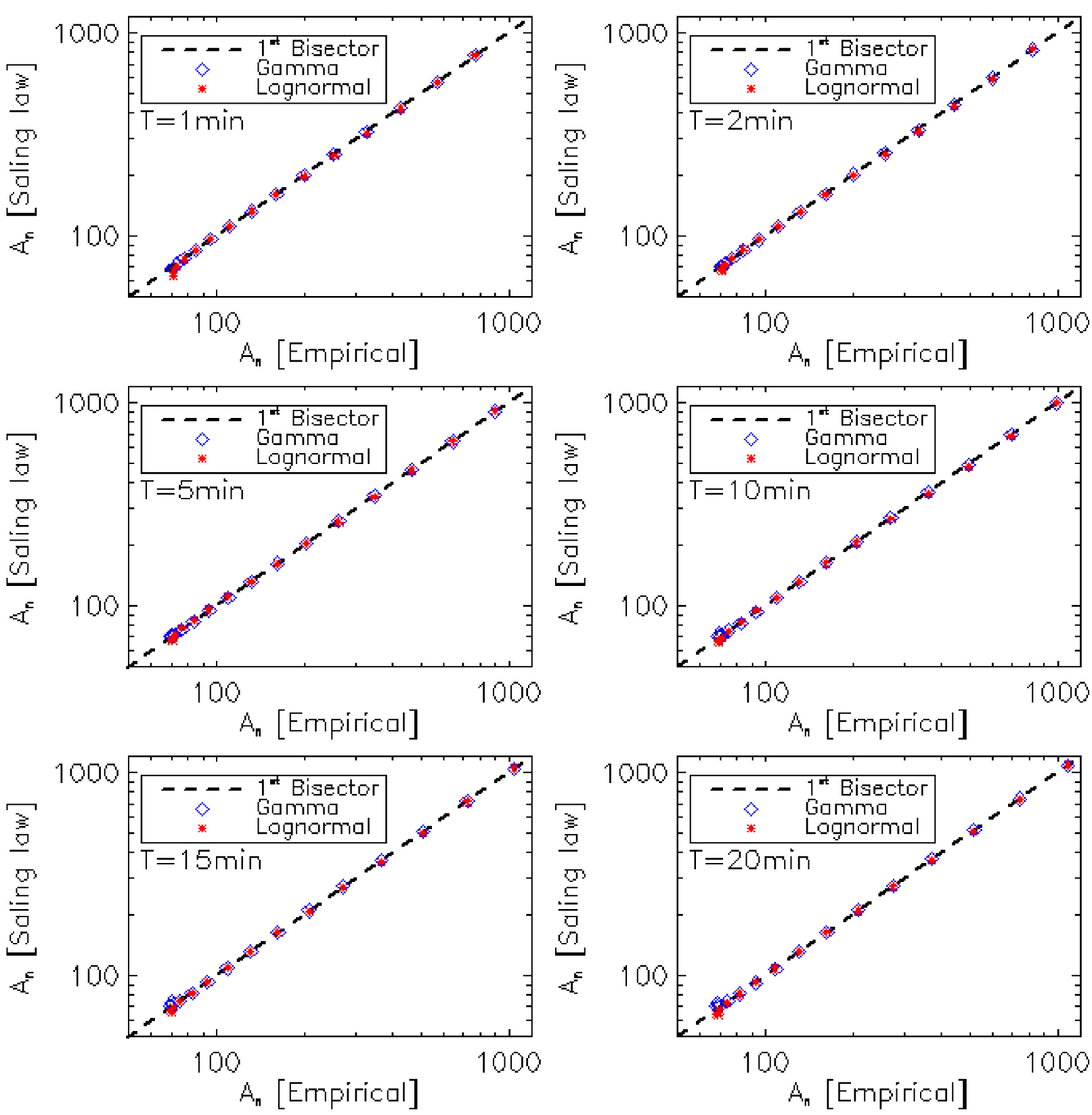
After estimating the parameters of the gamma (𝜇 and 𝜆) and lognormal (𝜎 and 𝜃) shape functions. The pre-factor A_n deduced from the formalism of the scaling law (relation (22) for gamma and relation (26) for lognormal) is represented as a function of the pre-factor A_n obtained by empirically method (Table 3), for the six integration time steps.

Figure 7.
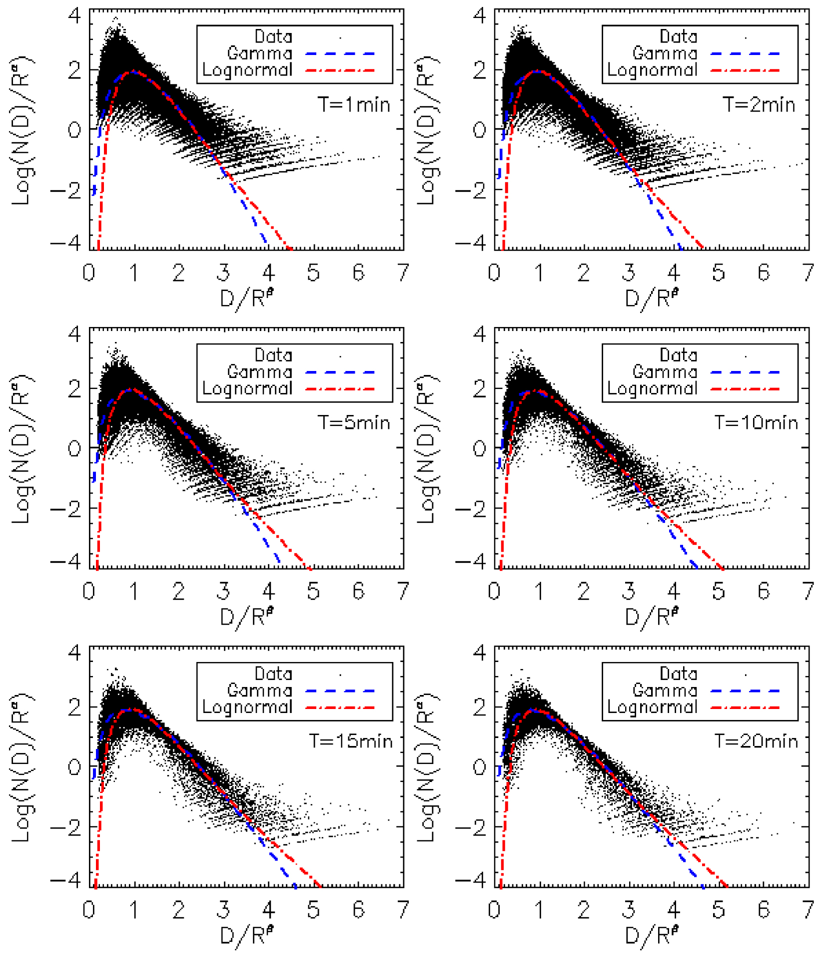
Representation of normalized spectra (relation (11)) and shape functions (gamma (relation (21)) and lognormal (relation (25))) for the six integration time steps.

We analysed the trend of the parameters entered in Table 4 with respect to the integration time steps. Figure 8 describes the adjustment of these parameters according to the integration time steps. Regarding the constants 𝛼 and 𝛽, their trends with regard to the measurement time are not significant. This justifies the very low dependence of the exponents b_n on the integration time steps. However, with the parameters of the shape functions (𝜇, 𝜆, 𝜎, and 𝜃), the trends in relation to the measurement duration are significant. This trend is clear: decreasing for 𝜇, 𝜆 and 𝜃; and increasing for 𝜎. These relations are registered in Table 5. Thus, the sensitivity of the pre-factors A_n with respect to the integration time steps is explained: for the gamma DSD model by the sensitivity of the parameters 𝜇 and 𝜆 with respect to the integration time steps; and for the lognormal DSD model by the sensitivity of the parameters 𝜎 and 𝜃 with respect to the integration time steps. Although Chapon et al. [2008] did not insist on this, we note in their article that the parameters (𝜇 and 𝜆) of the gamma distribution decrease as a function of the duration of measurement of the rain DSDs in agreement with our results.

Figure 8.
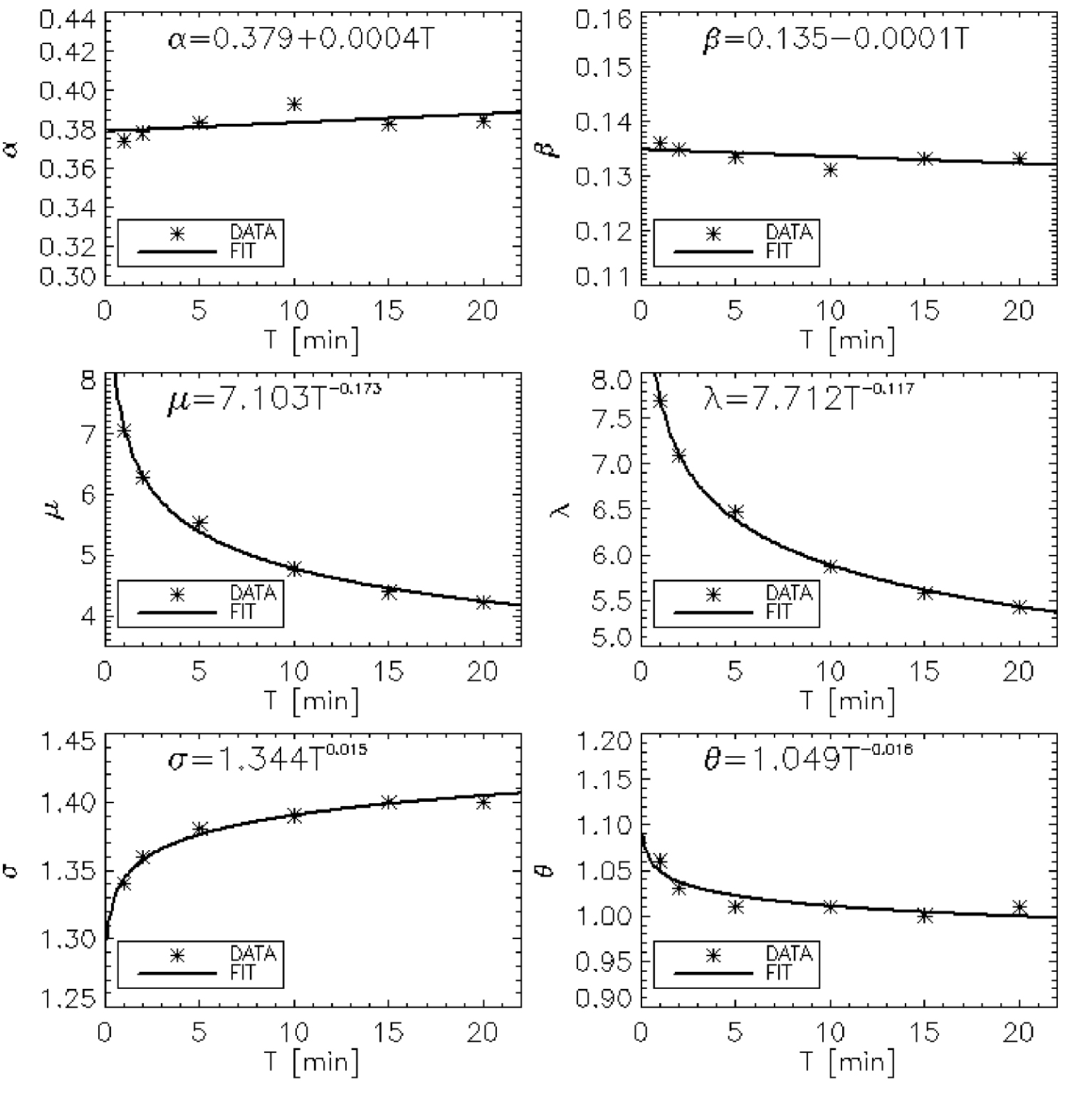
Trend of the constants (𝛼 and 𝛽), and trend of the parameters of the shape functions gamma (𝜇 and 𝜆), and lognormal (𝜎 and 𝜃) as a function of the integration time steps.

Integration time steps	Constants		Gamma DSD model		Lognormal DSD model
	𝛼	𝛽	𝜇	𝜆	𝜎	𝜃
T = 1 min	0.374	0.136	7.050	7.690	1.340	1.060
T = 2 min	0.378	0.135	6.270	7.090	1.360	1.030
T = 5 min	0.383	0.133	5.520	6.470	1.380	1.010
T = 10 min	0.393	0.131	4.770	5.870	1.390	1.010
T = 15 min	0.383	0.133	4.390	5.580	1.400	1.000
T = 20 min	0.384	0.133	4.220	5.430	1.400	1.010

Gamma DSD model	Lognormal DSD model
𝜇 = 7.103T^−0.173	𝜎 = 1.344T^0.015
𝜆 = 7.712T^−0.117	𝜃 = 1.049T^−0.016

We analysed the capacity of the models built to reproduce the moments of order n of the rain DSD. To estimate these moments, we used as input variables the measured rain rate, constants, and parameters listed in Table 4. The estimated moments are then compared with the measured moments using the statistical criteria defined in the Appendix. The results of this validation are described in Figures 9 and 10, respectively, for the gamma DSD model and the lognormal DSD model. These results show that there is no significant difference between the gamma DSD model, and the lognormal DSD model, for the estimation of the moments of the rain DSDs. Overall, the precision on the estimation of the moments is slightly improved with the increase in the measurement time of the spectra. This also proves that the relationships of a given integration time step cannot be used for another.

Figure 9.
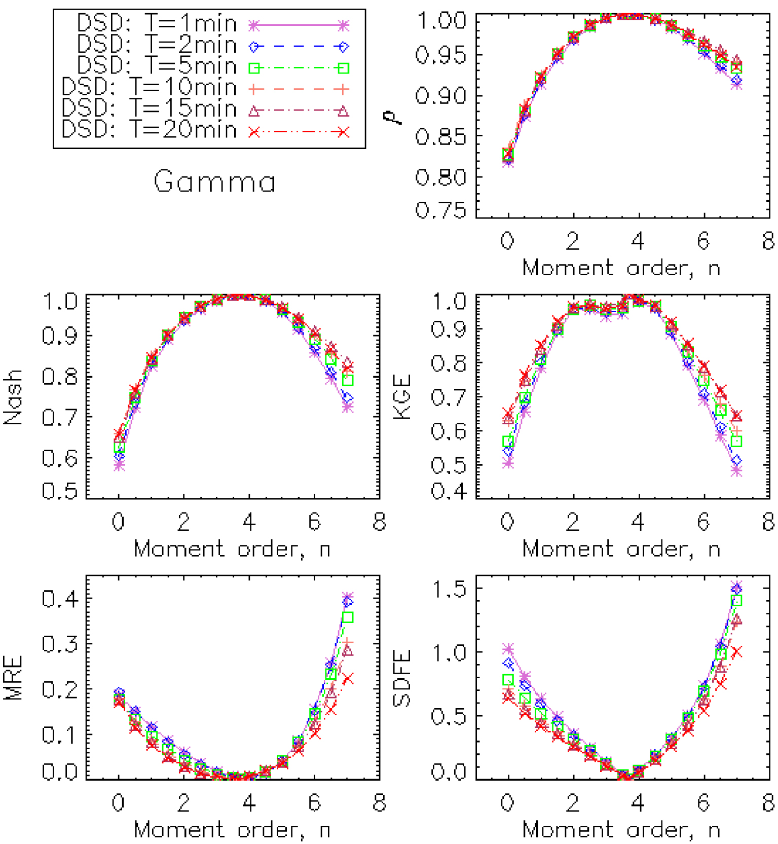
Validation of the fitting of the gamma DSD model: Statistical criteria calculated by comparing the moments measured with the moments estimated by the model.

Figure 10.
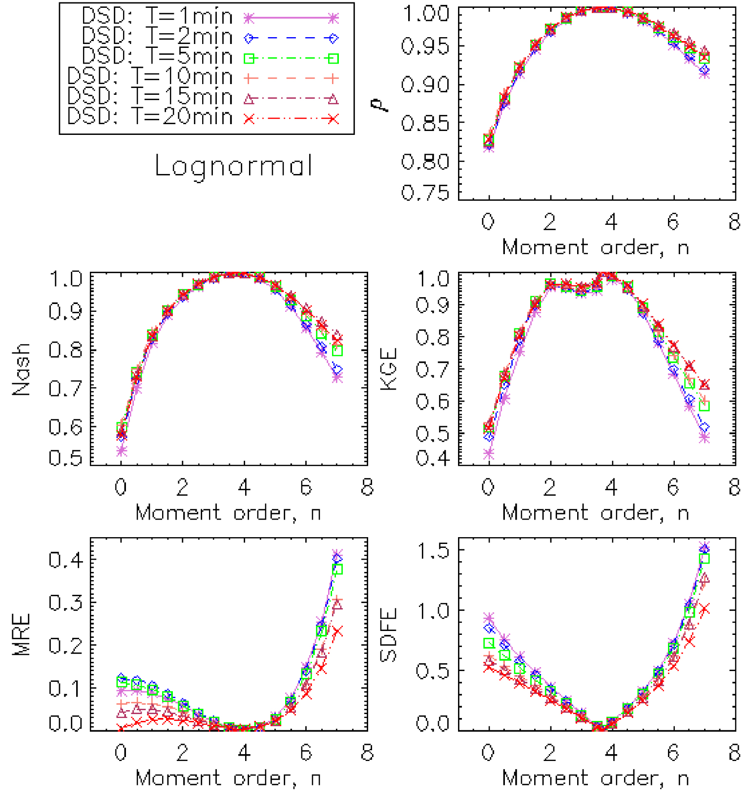
Validation of the fitting of the lognormal DSD model: Statistical criteria calculated by comparing the moments measured with the moments estimated by the model.

5. Discussion

In this paper, we obtained a maximum of 15% of spectra ill adjusted by a unimodal DSD model, of integration time T = 1 min, with the efficiency criteria Nash < 0.6 or KGE < 0.6, and this proportion decreases according to the duration of integration. To our knowledge, there are no reference, in relation to our analysis, allowing us to make a comparison. It is nevertheless obvious that this proportion must vary according to the threshold of the criteria. In addition, it would be very interesting to research, in further work, the possible link between the number of multimodal spectra and the efficiency criteria of their modelling.

Several studies on rain DSDs have parameterized rain DSD using the scaling law formalism proposed by Sempere-Torres et al. [1994] mainly [Chapon et al. 2008; Lee et al. 2004; Sempere Torres et al. 1998].

Ochou et al. [2007] used the same method as Sauvageot and Lacaux [1995] and they formalize this method. They applied this method to the rain DSDs measured with the JW-Disdrometer [JW means Joss and Waldvogel 1969]. These data are collected, at different years, at four West African sites. Comparison of our results with those of Ochou et al. [2007] needs establishment of new relationships. Then, using (10), (12), (14) and (26), we obtained

\begin{matrix} N_{T} = A_{0} R^{𝛼 + 𝛽} and D_{g} = 𝜃 R^{𝛽} \end{matrix}

(27)

Using (27) and making an identification with the relations of Ochou et al. [2007], we obtained the values reported in Table 6. It is noted that the constants and the parameters obtained in this article are well in line with those obtained in the West African region [Ochou et al. 2007]. It can also be noted that the constants $𝛼$ and 𝛽 for the West African region (tropical zone) clearly differ from those obtained in Cévennes-Vivarais (France) [Chapon et al. 2008]. It would therefore be interesting to extend this study to several climatic regions.

No.	Locality	Constants		Gamma DSD model		Lognormal DSD model		Author
		𝛼	𝛽	𝜇	𝜆	𝜎	𝜃
1	Djougou (Bénin)	0.375	0.136	7.090	7.740	1.330	1.080	This paper
2	Abidjan (Côte d’Ivoire)	0.440	0.120	—	—	1.340	1.000	Ochou et al. [2007]
3	Boyélé (Congo)	0.310	0.150	—	—	1.410	0.970	Ochou et al. [2007]
4	Dakar (Sénégal)	0.520	0.100	—	—	1.410	0.960	Ochou et al. [2007]
5	Niamey (Niger)	0.440	0.120	—	—	1.490	0.950	Ochou et al. [2007]
6	West Africa (No. 2 + 3 + 4 + 5)	0.420	0.120	—	—	1.410	0.970	Ochou et al. [2007]
7	Cévennes-Vivarais (France)	0.089	0.195	5.00	7.93	—	—	Chapon et al. [2008]

6. Concluding remarks

In the same logic as [Chapon et al. 2008], we have studied in this work the sensitivity of the parameterization of the rain DSD by the rain rate, according to the integration time step of the rain DSD (duration T of spectrum measurement). From the 1 min rain DSDs measured in the North of Benin (West Africa), five other datasets of different integration time step were generated. The spectra of each dataset are individually adjusted by gamma or lognormal DSD models. The efficiency of these models, measured using two statistical criteria (Nash and KGE), is used to characterize the structuring of the spectra. Analysis of the occurrence statistics of the structuring of the spectra reveals that spectra ill adjusted by a unimodal DSD model represent 5 to 15% of the population of 1 min rain DSDs. This population decreases according to the duration of measurement of the spectra. This result is in agreement with those of Chapon et al. [2008] who noted that the rain DSD spectra are better organized according to their duration of measurement.

The superimposed rain DSDs of each dataset are parameterized by the rain rate, using the scaling law formalism developed by Sempere-Torres et al. [1994]. It was also shown that the parameters of the shape functions (gamma and lognormal) have a significant tendency with respect to the integration time step of the rain DSDs. The effectiveness of this parameterization was evaluated by comparing the estimated useful moments with the measured useful moments. Furthermore, results show that the pre-factors of the relationships between the moments of the rain DSD and the rain rate, increase as a function of the duration of measurement of the spectra. This growth is explained by the trend of the parameters of the shape functions with respect to the integration time step of the rain DSDs.

The modelling of rain DSDs is of great use for several applications: quantitative estimation of rain by weather radars or by mobile telecommunication links; forecasting the attenuation of satellite signals by rain; leaching of atmospheric particles by rain; soil erosion by rain; etc. The results of this work will have important consequences for all these applications. For the study of soil erosion by rain, we recommend the optimal integration time of 10 min, since the data generally used are from rain gauge networks. For weather radars, measurements are quasi-instantaneous and available each 5 or 10 min; we recommend algorithms with integration times of less than 1 min. This is theoretically possible with the relationships in Table 5.

Bibliographie

[Atlas and Ulbrich, 1977] D. Atlas; C. W. Ulbrich Path and area-integrated rainfall measurement by microwave attenuation in the 1–3 cm band, J. Appl. Meteorol., Volume 16 (1977), pp. 1322-1331 | DOI

[Atlas et al., 1999] D. Atlas; C. W. Ulbrich; F. D. Marks Jr; E. Amitai; C. R. Williams Systematic variation of drop size and radar-rainfall relations, J. Geophys. Res., Volume 104 (1999), pp. 6155-6169 | DOI

[Cerro et al., 1997] C. Cerro; B. Codina; J. Bech; J. Lorente Modeling raindrop size distribution and Z(R) relations in the western Mediterranean area, J. Appl. Meteorol., Volume 36 (1997), pp. 1470-1479 | DOI

[Chapon et al., 2008] B. Chapon; G. Delrieu; M. Gosset; B. Boudevillain Variability of rain drop size distribution and its effect on the Z–R relationship: A case study for intense Mediterranean rainfall, Atmos. Res., Volume 87 (2008), pp. 52-65 | DOI

[Chen et al., 2019] Y. Chen; J. Duan; J. An; H. Liu Raindrop size distribution characteristics for tropical cyclones and Meiyu-Baiu fronts impacting Tokyo, Japan, Atmosphere, Volume 10 (2019), 391 | DOI

[Delahaye et al., 2005] J.-Y. Delahaye; L. Barthès; P. Golé; J. Lavergnat; J. P. Vinson A dual-beam spectropluviometer concept, J. Hydrol., Volume 328 (2005), pp. 110-120 | DOI

[Ekerete et al., 2015a] K. E. Ekerete; F. H. Hunt; J. L. Jeffery; I. E. Otung Modelling rainfall drop size distributions in southern England using a Gaussian mixture model, Radio Sci., Volume 50 (2015a), pp. 876-885 | DOI

[Ekerete et al., 2015b] K.-M. E. Ekerete; F. H. Hunt; I. E. Otung; J. L. Jeffery Multimodality in the rainfall drop size distribution in southern England, Wireless and Satellite Systems: 7th International Conference, WiSATS 2015, Bradford, UK, July 6–7, 2015, Revised Selected Papers (2015b), pp. 177-184 | DOI

[Ekerete et al., 2016] K. E. Ekerete; F. H. Hunt; J. L. Jeffery; I. Otung Variation of multimodality in rainfall drop size distribution with wind speeds and rain rates, J. Eng., Volume 6 (2016), pp. 203-209 | DOI

[Feingold and Levin, 1986] G. Feingold; Z. Levin The lognormal fit of raindrop spectra from frontal convective clouds in Israel, J. Climatol. Appl. Meteorol., Volume 25 (1986), pp. 1346-1363 | DOI

[Gosset et al., 2010] M. Gosset; E. P. Zahiri; S. Moumouni Rain drop size distributions variability and impact on Xband polarimetric radar retrieval: results from the AMMA campaign in Benin, Q. J. R. Meteorol. Soc., Volume 136 (2010), pp. 243-256 | DOI

[Gupta et al., 2009] H. V. Gupta; H. Kling; K. K. Yilmaz; G. F. Martinez Decomposition of the mean squared error and NSE performance criteria: implications for improving hydrological modelling, J. Hydrol., Volume 377 (2009), pp. 80-91 | DOI

[Joss and Waldvogel, 1969] J. Joss; A. Waldvogel Raindrop size distribution and sampling size errors, J. Atmos. Sci., Volume 26 (1969), pp. 566-569 | DOI

[Kougbéagbédè et al., 2017] H. Kougbéagbédè; B. E. Houngninou; S. Moumouni Modeling rain rate distribution per diameter class from disdrometer data collected in northern Benin (AMMA Campaign): a new relationship between radar reflectivity and rainfall rate, Int. J. Res. Innov. Earth Sci., Volume 4 (2017) no. 3, p. 2394-1375 (Online)

[Lee et al., 2004] G. W. Lee; I. Zawadzki; W. Szyrmer; D. Sempere-Torres; R. A. Uijlenhoet Genaral approch to double-moment normalisation of drop size distributions, J. Appl. Meteorol., Volume 43 (2004), pp. 264-281 | DOI

[Löffler-Mang and Joss, 2000] M. Löffler-Mang; J. Joss An optical disdrometer for measuring size and velocity of hydrometeors, J. Atmos. Oceanic. Technol., Volume 17 (2000), pp. 130-139 | DOI

[Maki et al., 2001] M. Maki; T. D. Keenan; Y. Sasaki; K. Nakamura Characteristics of the raindrop size distribution in tropical continental squall lines observed in Darwin, Australia, J. Appl. Meteorol., Volume 40 (2001), pp. 1393-1412 | DOI

[Marshall and Palmer, 1948] J. S. Marshall; W. McK. Palmer The distribution of raindrop with size, J. Meteorol., Volume 5 (1948), pp. 165-166 | DOI

[Moumouni et al., 2008] S. Moumouni; M. Gosset; E. Houngninou Main features of rain drop size distributions observed in Benin, West Africa, with optical disdromètres, Geophys. Res. Lett., Volume 35 (2008), L23807 | DOI

[Moumouni et al., 2018] S. Moumouni; L. S. Adjikpé; S. Massou; A. E. Lawin Parameterization of drop size distribution with rainfall rate: comparison of the N(D) and R(D) functions; and relationship between gamma and lognormal laws, Int. J. Res. Innov. Earth Sci., Volume 5 (2018) no. 6, p. 2394-1375 (Online)

[Moumouni, 2009] S. Moumouni Analyse des distributions granulométriques des pluies au Bénin : caractéristiques globales, variabilité et application à la mesure radar, Ph. D. Thesis, INP-Grenoble, France (2009) (191 p.)

[Nash and Sutcliffe, 1970] J. E. Nash; J. V. Sutcliffe River flow forecasting through conceptual models part I—A discussion of principles, J. Hydrol., Volume 10 (1970), pp. 282-290 | DOI

[Nzeukou et al., 2004] A. Nzeukou; H. Sauvageot; A. D. Ochou; C. M. F. Kebe Raindrop size distribution and radar parameters at Cape Verde, J. Appl. Meteorol., Volume 43 (2004), pp. 90-105 | DOI

[Ochou et al., 2007] A. D. Ochou; A. Nzeukou; H. Sauvageot Parametrization of drop size distribution with rain rate, Atmos. Res., Volume 84 (2007), pp. 58-66 | DOI

[Radhakrisna and Narayana Rao, 2009] B. Radhakrisna; T. Narayana Rao Statistical characteristics of multipeak raindrop size distributions at the surface, and aloft in different rain regimes, Mon. Weather Rev., Volume 137 (2009), pp. 3501-3518 | DOI

[Salles et al., 1998] C. Salles; J. D. Creutin; D. Sempere-Torres The optical spectropluviometer revisited, J. Atmos. Oceanic. Technol., Volume 15 (1998), pp. 1215-1222 | DOI

[Salles, 1995] C. Salles Analyse microphysique de la pluie au sol: Mesures par spectropluviomètre optique et méthodes statistiques d’analyse spectrale et de simulation numérique, Ph. D. Thesis, Université Joseph Fourier, Grenoble, France (1995) (212 p.)

[Sauvageot and Koffi, 2000] H. Sauvageot; M. Koffi Multimodal raindrop size distribution, J. Atmos. Sci., Volume 57 (2000), pp. 2480-2492 | DOI

[Sauvageot and Lacaux, 1995] H. Sauvageot; J. P. Lacaux The shape of averaged drop size distributions, J. Atmos. Sci., Volume 52 (1995), pp. 1070-1083 | DOI

[Sempere-Torres et al., 1994] D. J. Sempere-Torres; M. Porra; J. D. Creutin A general formulation for raindrop size distribution, J. Appl. Meteorol., Volume 33 (1994), pp. 1494-1502

[Sempere Torres et al., 1998] D. Sempere Torres; J. M. Porra; J. D. Creutin Experimental evidence of a general description for raindrop size distribution properties, J. Geophys. Res., Volume 103 (1998), pp. 1785-1797 | DOI

[Steiner and Waldvogel, 1987] M. Steiner; A. Waldvogel Peaks in raindrop size distributions, J. Atmos. Sci., Volume 44 (1987), pp. 3127-3133 | DOI

[Tenorio et al., 2012] R. S. Tenorio; M. C. da Silva Moraes; H. Sauvageot Raindrop size distribution and radar parameters in coastal tropical rain systems of northeastern Brazil, J. Appl. Meteorol. Climatol., Volume 51 (2012), pp. 1960-1970 | DOI

[Testud et al., 2001] J. Testud; S. Oury; R. A. Black; P. Amayenc; X. Dou The concept of “normalized” distribution to describe raindrop spectra: A tool for cloud physics and cloud remote sensing, J. Appl. Meteorol., Volume 40 (2001), pp. 1118-1140 | DOI

[Tokay and Short, 1996] A. Tokay; D. A. Short Evidence from tropical raindrop spectra of the origin of rain from stratiform versus convective clouds, J. Appl. Meteorol., Volume 35 (1996), pp. 355-371 | DOI

[Uijlenhoet et al., 2003] R. Uijlenhoet; J. A. Smith; M. Steiner The microphysical structure of extreme precipitation as inferred from ground-based raindrop spectra, J. Atmos. Sci., Volume 60 (2003), pp. 1220-1238 | DOI

[Ulbrich and Atlas, 1998] C. W. Ulbrich; D. Atlas Rainfall microphysics and radar properties: Analysis methods for drop size spectra, J. Appl. Meteorol., Volume 37 (1998), pp. 912-923 | DOI

[Ulbrich, 1983] C. W. Ulbrich Natural variation in the analytical form of the raindrop size distribution, J. Climatol. Appl. Moteorol., Volume 22 (1983), pp. 1764-1775 | DOI

[Wen et al., 2018] L. Wen; K. Zhao; G. Chen; M. Wang; B. Zhou; H. Huang; D. Hu; W.-C. Lee; H. Hu Drop size distribution characteristics of seven typhoons in China, J. Geophys. Res. Atmos., Volume 123 (2018), pp. 6529-6548 | DOI

[Willis, 1984] P. T. Willis Functional fits to some observated drop size distributions and parametrisation of rain, J. Atmos. Sci., Volume 41 (1984), pp. 1648-1661 | DOI

[Zeng et al., 2019] Q. Zeng; Y. Zhang; H. Lei; Y. Xie; T. Gao; L. Zhang; C. Wang; Y. Huang Microphysical characteristics of precipitation during pre-monsoon, monsoon, and post-monsoon periods over the south China sea, Adv. Atmos. Sci., Volume 36 (2019), pp. 1103-1120 | DOI

[Zhang et al., 2003] G. Zhang; J. Vivekanandan; E. A. Brandes; R. Meneghini; T. Kozu The shape-slope relation in observed gamma raindrop size distributions: statistical error or useful information?, J. Atmos. Oceanic Technol., Volume 20 (2003), pp. 1106-1119 | DOI

Commentaires - Politique

Ces articles pourraient vous intéresser

Impact of integration time steps of rain drop size distribution on their double-moment normalization: a case study in northern Benin

Sounmaïla Moumouni; Fulgence Payot Akponi; Eric-Pascal Zahiri; ...

C. R. Géos (2023)

Laser diode reliability: crystal defects and degradation modes

Juan Jiménez

C. R. Phys (2003)

Risk-averse estimates of effective properties in heterogeneous elasticity

Jeremy Bleyer

C. R. Méca (2023)