Assessing heterotopic searching strategy in hierarchical cosimulation for modeling the variables with inequality constraints

Sultan Abulkhair; Nasser Madani

doi:10.5802/crgeos.58

Article original - Pétrologie, Géochimie

Assessing heterotopic searching strategy in hierarchical cosimulation for modeling the variables with inequality constraints

Sultan Abulkhair ¹ ; Nasser Madani ¹

¹ School of Mining and Geosciences, Nazarbayev University, Nur-Sultan city, Kazakhstan

Comptes Rendus. Géoscience, Volume 353 (2021) no. 1, pp. 115-134.

Résumé

A hierarchical sequential Gaussian cosimulation method is applied in this study for modeling the variables with an inequality constraint in the bivariate relationship. An algorithm is improved by embedding an inverse transform sampling technique in the second simulation to reproduce bivariate complexity and accelerate the process of cosimulation. A heterotopic simple cokriging (SCK) is also proposed, which introduces two moving neighborhoods: single and multiple searching strategies in both steps of the hierarchical process. The proposed algorithm is tested over a real case study from an iron deposit where iron and aluminum oxide shows a strong bivariate dependency as well as a sharp inequality constraint. The results showed that the proposed hierarchical cosimulation with a multiple searching strategy provides satisfying results compared to the case when a single searching strategy is employed. Moreover, the proposed algorithm is compared to the conventional hierarchical cosimulation, which does not implement the inverse transform sampling integrated into the second simulation. The proposed methodology successfully reproduces inequality constraint, while conventional hierarchical cosimulation fails in this regard. However, it is demonstrated that the proposed methodology requires further improvement for better reproduction of global statistics (i.e., mean and standard deviation).

Métadonnées

Reçu le : 2021-01-30
Révisé le : 2021-04-03
Accepté le : 2021-04-29
Publié le : 2021-05-27

DOI : 10.5802/crgeos.58

Mots clés : Multivariate geostatistics, Inequality constraint, Cosimulation, Heterotopic sampling, Cokriging neighborhood, Carajas mine

Affiliations des auteurs :

Sultan Abulkhair ¹ ; Nasser Madani ¹

¹ School of Mining and Geosciences, Nazarbayev University, Nur-Sultan city, Kazakhstan

Licence :

CC-BY 4.0

Droits d'auteur : Les auteurs conservent leurs droits

@article{CRGEOS_2021__353_1_115_0,
     author = {Sultan Abulkhair and Nasser Madani},
     title = {Assessing heterotopic searching strategy in hierarchical cosimulation for modeling the variables with inequality constraints},
     journal = {Comptes Rendus. G\'eoscience},
     pages = {115--134},
     publisher = {Acad\'emie des sciences, Paris},
     volume = {353},
     number = {1},
     year = {2021},
     doi = {10.5802/crgeos.58},
     language = {en},
}

TY  - JOUR
AU  - Sultan Abulkhair
AU  - Nasser Madani
TI  - Assessing heterotopic searching strategy in hierarchical cosimulation for modeling the variables with inequality constraints
JO  - Comptes Rendus. Géoscience
PY  - 2021
SP  - 115
EP  - 134
VL  - 353
IS  - 1
PB  - Académie des sciences, Paris
DO  - 10.5802/crgeos.58
LA  - en
ID  - CRGEOS_2021__353_1_115_0
ER  -

%0 Journal Article
%A Sultan Abulkhair
%A Nasser Madani
%T Assessing heterotopic searching strategy in hierarchical cosimulation for modeling the variables with inequality constraints
%J Comptes Rendus. Géoscience
%D 2021
%P 115-134
%V 353
%N 1
%I Académie des sciences, Paris
%R 10.5802/crgeos.58
%G en
%F CRGEOS_2021__353_1_115_0

Sultan Abulkhair; Nasser Madani. Assessing heterotopic searching strategy in hierarchical cosimulation for modeling the variables with inequality constraints. Comptes Rendus. Géoscience, Volume 353 (2021) no. 1, pp. 115-134. doi : 10.5802/crgeos.58. https://comptes-rendus.academie-sciences.fr/geoscience/articles/10.5802/crgeos.58/

Version originale du texte intégral (Proposez une traduction )

1. Introduction

Multivariate geostatistics is an essential tool for resource modeling in the presence of moderate or strong correlation between coregionalized variables [Goovaerts 1997; Chilès and Delfiner 2012; Pyrcz and Deutsch 2014; Rossi and Deutsch 2014]. Recent industry requirements for uncertainty quantification motivate the use of stochastic cosimulation instead of deterministic cokriging estimation methods. The most widely used cosimulation approaches are based on multi-Gaussian assumptions such as turning bands cosimulation [Emery 2008] and sequential Gaussian cosimulation [Verly 1993; Tran 1994]. One drawback of these traditional cosimulation techniques is that they cannot reproduce complexities in the bivariate relationships between variables, such as nonlinearity, heteroscedasticity, and geological constraints. Alternatively, implementation of geostatistical factorization, namely projection pursuit multivariate transform [Barnett et al. 2014, 2016], flow anamorphosis [van den Boogaart et al. 2017], among others, are designed to deal with complexities. However, these factorization methods have difficulty in reproducing geological inequality constraints present in bivariate relationships. Modeling of variables with inequality constraints has been attempted by using stepwise conditional transformation [Leuangthong and Deutsch 2003], minimum/maximum autocorrelation factor [Desbarats and Dimitrakopoulos 2000; Vargas-Guzmán and Dimitrakopoulos 2003] with changing to new variables free of inequality constraint [Abildin et al. 2019], log-ratio transformation [Pawlowsky-Glahn and Olea 2004; Pawlowsky-Glahn and Egozcue 2006], projection pursuit multivariate transform on variables changed into ratios [Arcari Bassani et al. 2018] and stoichiometric relations of original variables [Mery et al. 2017; Adeli et al. 2018]. One significant limitation of these factorization algorithms is that they can be applied mostly on isotopic data sets, wherever the sample observations of variables are required to share the exact locations. Another impediment of some of these approaches is that the marginal distributions of both cross-correlated variables should be identical.

Another method of modeling variables with inequality constraints is to use hierarchical sequential Gaussian cosimulation integrated with an acceptance–rejection technique [Madani and Abulkhair 2020]. This algorithm enables simulating values iteratively in order to meet the requirements that are imposed by an inequation. The method works with any bivariate marginal distributions and any sampling patterns, including partially and entirely heterotopic. However, there are two issues with this algorithm. The first one is related to the acceptance–rejection methodology that acts as a speed bump in the cosimulation procedure. The second one is related to the definition of the searching neighborhood, which is based on a heterotopic simple cokriging in the first step and multicollocated cokriging in the second step of this hierarchy. Although these two neighborhood strategies are satisfying in terms of global and local reproduction of statistical parameters, using other types of moving neighborhoods might also be of interest. In this research, to come up with the first difficulty, an inverse transformation sampling is substituted for the acceptance–rejection method to accelerate the process of cosimulation. In addition, a heterotopic SCK is also embedded into the algorithm as a replacement of the multicollocated cokriging. This type of SCK allows attending more data in the established neighborhood, which boosts the simulation quality. For this purpose, single and multiple searching strategies are introduced and examined in the hierarchical cosimulation algorithm proposed.

The paper proceeds as follows: (1) Proposed methodology of hierarchical cosimulation is described. (2) Presentation of a real case study from Carajas mine with a bivariate data set of iron and aluminum oxide grades. (3) Exploratory data analysis and multi-Gaussianity check of the data set. (4) Cosimulation using both methodologies (i.e., proposed and conventional) with single and multiple search strategies. (5) Comparison of methods in terms of reproduction of mean, standard deviation, correlation coefficient, bivariate relationship, direct- and cross-variograms. (6) Conclusion with recommendations for future work.

2. Methodology

In this study, the proposed algorithm is inspired by a hierarchical cosimulation algorithm integrated with an acceptance–rejection technique developed by Madani and Abulkhair [2020]. Traditional hierarchical sequential Gaussian cosimulation [Almeida and Journel 1994] is different from traditional cosimulation in terms of the simulation process. In the case of a bivariate data set, hierarchical cosimulation proceeds in two stages: (1) it simulates the primary variable in the entire region, (2) it simulates the secondary variable accounting to previously simulated values using collocated cokriging. The selection of primary and secondary variables can depend on their availability in the case of a partially heterotopic sampling pattern [Wackernagel 2003]. However, if the sampling pattern is isotopic, a variable with better spatial continuity is selected as the primary variable [Goovaerts 1997]. The following sections contain background information on different types of inequality constraints, the methodology of the algorithm developed by Madani and Abulkhair [2020], and main improvements of the proposed algorithm, including an inverse transform sampling and heterotopic searching strategies. Throughout the paper, the conventional hierarchical sequential Gaussian cosimulation refers to the algorithm with the same searching strategies but without inverse transform sampling integrated into the second simulation.

2.1. Inequality constraints over the bivariate relationship

In multivariate modeling of coregionalized variables, it is common to deal with some type of inequality or equality constraints. Generally, there are three types of such constraints in the bivariate relationship in the case of denoting the primary variable as Z₁ and secondary variable as Z₂:

Strict inequality constraint is related to the cases where the secondary variable is either less than (Z₂ < Z₁) or greater than (Z₂ > Z₁) the primary variable.
Nonstrict inequality constraint is similar to the previous one. However, in this case, bivariate relationship is not restricted, thus the secondary variable can be less than, greater than or equal to the primary variable. Such a relationship can be expressed in the following fashion: Z₂⩽Z₁ or Z₂⩾Z₁.
Inequality constraint is expressed by an inequation, which can be linear or any other type. For example, when dealing with linear inequation with slope w and intercept b, the bivariate relationship is expressed by Z₂ < wZ₁ + b or Z₂ > wZ₁ + b for strict cases, Z₂⩽wZ₁ + b or Z₂⩾wZ₁ + b for nonstrict cases.

This paper focuses on the third type of inequality constraints, which can be modeled using the following algorithms of a hierarchical cosimulation.

2.2. Hierarchical cosimulation with inequality constraint

Madani and Abulkhair [2020] proposed an adapted algorithm for geostatistical modeling of variables with inequality constraints using a hierarchical cosimulation framework. This approach made several modifications to the original algorithm by integrating an acceptance–rejection method to simulate the linear constraint in the bivariate relationship; by implementing SCK to simulate the primary variable and simple multicollocated cokriging (SMCCK) for the secondary variable. The steps are described as follows:

2.3. Proposed cosimulation algorithm

In this study, we propose an alternative of this hierarchical cosimulation algorithm for modeling variables with inequality constraint where the acceptance–rejection method is replaced with an inverse transform sampling technique, which accelerates the algorithm. Another improvement is related to the searching neighborhood. For this, two searching strategies are examined that will be discussed in the subsequent sections.

2.3.1. Inverse transform sampling

Generating random numbers that follow a particular probability distribution is a core principle of statistics. One method for obtaining such random numbers is based on inverse transform sampling. This method can be summarized in three steps [Devroye 1986]: (1) calculate the cumulative distribution function (CDF); (2) generate the uniformly distributed random number between 0 and 1; and (3) compute the inverse CDF of the generated random number.

Inverse transform sampling can also be used to generate a random number in a predefined interval [Burkardt 2014]. If a target variable Z lies within two consecutive truncated thresholds [𝛼,𝛽], so that 𝛼⩽Z⩽𝛽, inverse transform sampling proceeds as follows [Devroye 1986]:

V = F^{- 1} (F (𝛼) + (F (𝛽) - F (𝛼)) \cdot U),

(3)

where

V

is random inverse transform, U is a random number distributed uniformly between 0 and 1, F is the conditioned CDF and F⁻¹ is its corresponding quantile function.

This method replaces the acceptance–rejection method [Madani and Abulkhair 2020] in the proposed algorithm. For this purpose, step 5 in Section 2.2 is modified to:

Back-transform simulated values of the primary variable $Y_{1}^{n} (x_{i})$ to the original units.
Obtain minimum and maximum thresholds according to the fitted inequation (Figure 1), so that ${Z_{2}^{n}}_{min} = min (Z_{2})$ and ${Z_{2}^{n}}_{max} = w Z_{1}^{n} (x_{i}) + b$ in the case of negative inequation, or ${Z_{2}^{n}}_{min} = w Z_{1}^{n} (x_{i}) + b$ and ${Z_{2}^{n}}_{max} = max (Z_{2})$ in the case of positive inequation.
Transform both ${Z_{2}^{n}}_{min}$ and ${Z_{2}^{n}}_{max}$ to normal scores ${Y_{2}^{n}}_{min}$ and ${Y_{2}^{n}}_{max}$ , making the minimum and maximum threshold for simulation of the target variable.
Among n realizations, find simulated values of the secondary variable $Y_{2}^{n}$ that lie outside computed thresholds. Store faulty values by indicating realizations as c.
Use the inverse transform sampling following a truncated distribution on the interval $[{Y_{2}^{c}}_{min}, {Y_{2}^{c}}_{max}]$ to calculate the secondary variable $Y_{2}^{c} (u_{i})$ for faulty values found in step (iv).
$Y_{2}^{c} (x_{i}) = {Y_{2}}_{SCK} (x_{i}) + \sqrt{𝜎_{SCK}^{2} (x_{i})} \cdot V_{2}^{c} (x_{i}),$ (4)
where $V_{2}^{c} (u_{i})$ is an independent random number generated within a truncation threshold for c faulty realizations.

Figure 1.
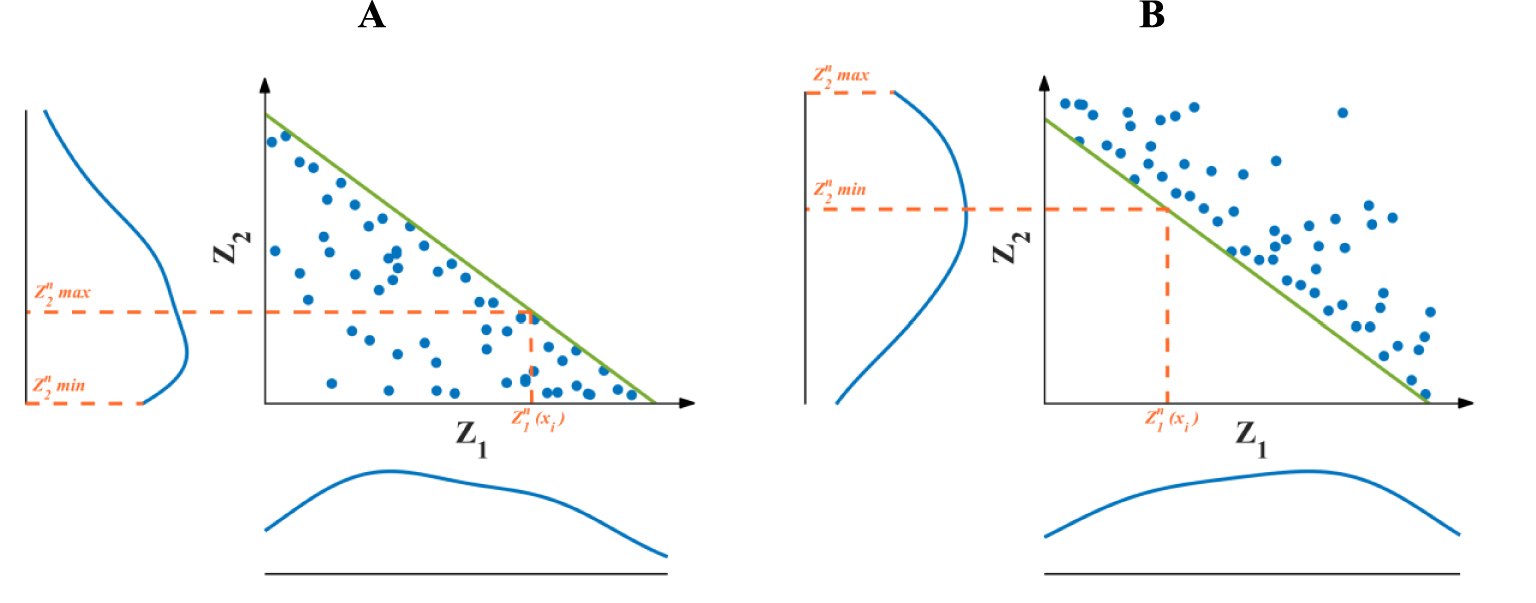
Obtaining minimum and maximum thresholds $[{Z_{2}^{m}}_{min}, {Z_{2}^{m}}_{max}]$ for the simulated value of secondary variable conditional to the simulated value of the primary variable $Z_{1}^{n} (u_{i})$ in the case of (A) negative and (B) positive inequations.

2.3.2. Definition of search strategies

In the hierarchical cosimulation algorithm, selecting an appropriate neighborhood strategy is of paramount importance because the secondary variable’s simulation is substantially impacted by the previously simulated values of the primary variable. In the algorithm described in Section 2.2, two searching strategies are identified. The first searching neighborhood involves a heterotopic SCK (i.e., single searching strategy), and the second one uses an SMCK. For the proposed methodology, however, heterotopic SCK is presented as an alternative. Simple cokriging estimator and estimation variance for the primary and secondary variables are the following:

\begin{matrix} {Y_{1}}_{SCK} (x_{0}) & = & m_{1} + \sum_{𝛼 = 1}^{n_{1}} w_{𝛼}^{1} [Y_{1} (x_{1, 𝛼}) - m_{1}] \\ + \sum_{𝛽 = 1}^{n_{2}} w_{𝛽}^{2} [Y_{2} (x_{2, 𝛽}) - m_{2}] \end{matrix}

(5)

\begin{matrix} {Y_{2}}_{SCK} (x_{0}) & = & m_{2} + \sum_{𝛼 = 1}^{n_{1}} w_{𝛼}^{1^{'}} [Y_{1} (x_{1, 𝛼}) - m_{1}] \\ + \sum_{𝛽 = 1}^{n_{2}} w_{𝛽}^{2^{'}} [Y_{2} (x_{2, 𝛽}) - m_{2}] \end{matrix}

(6)

\begin{matrix} {𝜎_{1}}_{SCK}^{2} (x_{0}) & = & C_{11} (x_{0} - x_{0}) - \sum_{𝛼 = 1}^{n 1} w_{𝛼}^{1} C_{11} (x_{1, 𝛼} - x_{0}) \\ - \sum_{𝛽 = 1}^{n 2} w_{𝛽}^{2} C_{21} (x_{2, 𝛽} - x_{0}) \end{matrix}

(7)

\begin{matrix} {𝜎_{2}}_{SCK}^{2} (x_{0}) & = & C_{22} (x_{0} - x_{0}) - \sum_{𝛼 = 1}^{n 1} w_{𝛼}^{1^{'}} C_{12} (x_{1, 𝛼} - x_{0}) \\ - \sum_{𝛽 = 1}^{n 2} w_{𝛽}^{2^{'}} C_{22} (x_{2, 𝛽} - x_{0}), \end{matrix}

(8)

where

w_{𝛼}^{1}

and

w_{𝛽}^{2}

are the weights assigned to the data of Y₁ and Y₂ at the 𝛼th and 𝛽th data locations, respectively; m₁ and m₂ are the mean values of variables Y₁ and Y₂, respectively; x_1,𝛼 (𝛼= 1,…,n₁) and x_2,𝛽 (𝛽= 1,…,n₂) are the data locations of primary Y₁ and secondary Y₂ variables, respectively; C₁₁ is the direct covariance of primary variable, C₁₁ is the direct covariance of secondary variable, C₂₁ and C₁₂ are the cross-covariances between Y₁ and Y₂; and x₀ is the target location for estimation.

Figure 2.
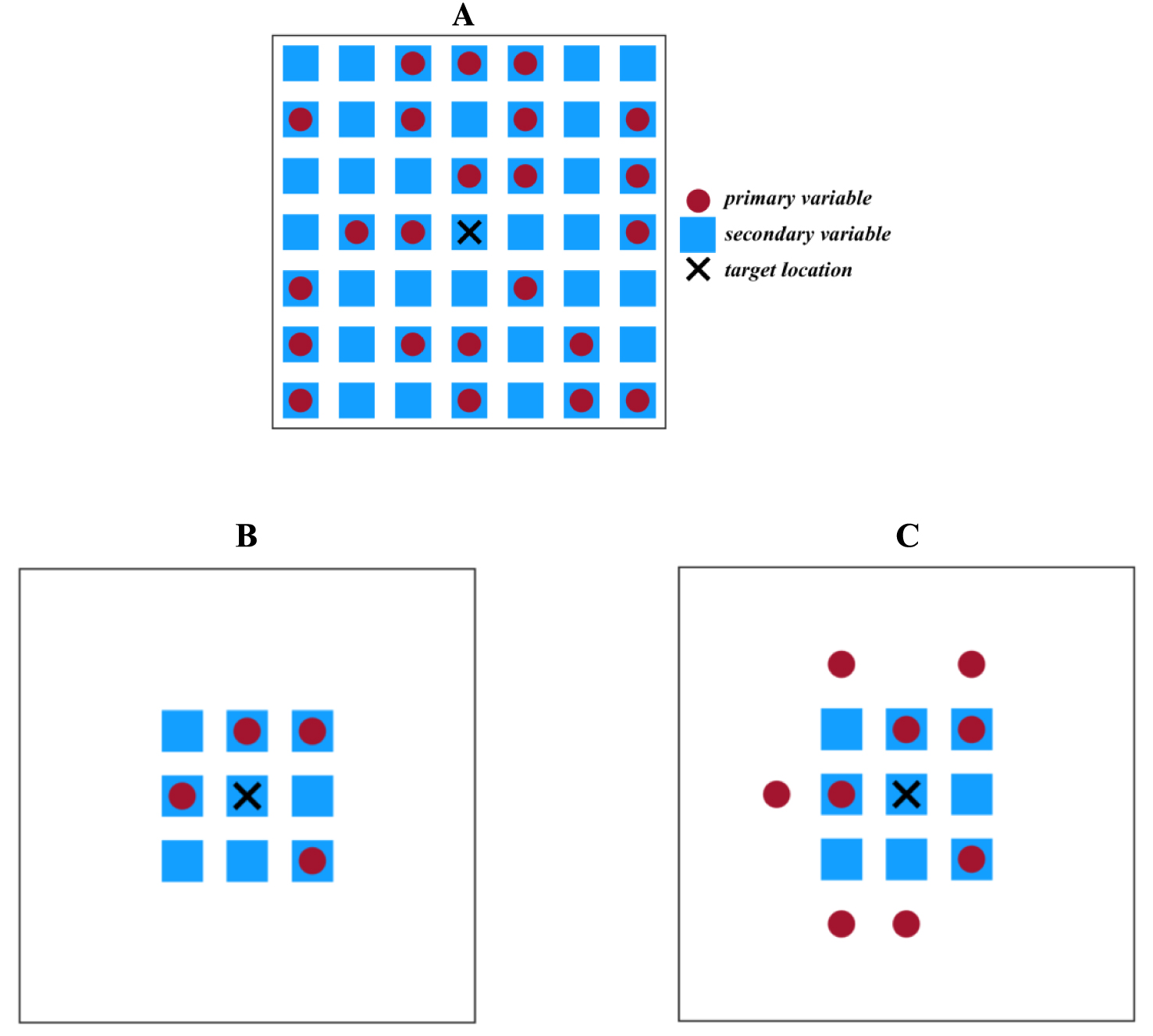
Schematic illustration of the (A) unique neighborhood, (B) single, and (C) multiple search strategies of moving neighborhood for nine closest data points.

For the searching of n1 and n2 samples of primary and secondary variables, two types of heterotopic searching strategy are offered in this study:

Single search: a neighborhood strategy that searches for n closest data locations, whether only one or both variables are known at these locations.
Multiple search: a neighborhood strategy that first searches for n closest data of primary variable, then it searches for the n closest data of secondary variable, irrespective of the primary variable.

Therefore, in this study, two cases are considered:

Case I: first and second searching strategies are both single.
Case II: first and second searching strategies are both multiple.

During the second run of hierarchical cosimulation, the previously simulated primary variable is exhaustively known at all locations, while the secondary variable is sparsely located. Figure 2 shows the schematic example of searching strategies listed above, where a unique search (Figure 2A) demonstrates the case of selecting all data points. Single search in a moving neighborhood (Figure 2B) selects nine closest data locations, which contain 9 secondary data points and only 4 primary data points. On the other hand, the multiple searching strategy (Figure 2C) first selects 9 data points of the primary and then 9 data points of the secondary variable. It can be clearly seen that in a multiple searching strategy, the neighborhood captures more data.

3. Results

3.1. Presentation of case study

Conventional and proposed hierarchical cosimulation algorithms integrated with single and multiple search strategies proposed in this study are applied to a real case study from the Carajas iron deposit. The study area is located in the municipality of Parauapebas, Para state, Northern Brazil, about 550 km from Belem city. A geological map with a stratigraphic sheet is given in Figure 3. The geological formation of the deposit is characterized by volcanic rocks of the Parauapebas formation [Meireles et al. 1984] and metasedimentary ironstones of the Carajas formation [Beisiegel et al. 2018]. Carajas iron deposit is composed of heterogeneous and anisotropic rock masses with different shear strength values [BVP 2011]. This deposit is considered as one of the largest iron ore mines, with a high concentration of iron-bearing formations, such as mafic rocks and ironstones. The latter is classified into jaspilite, soft hematite, hard hematite, and low-grade iron ore [Paradella et al. 2015].

Figure 3.
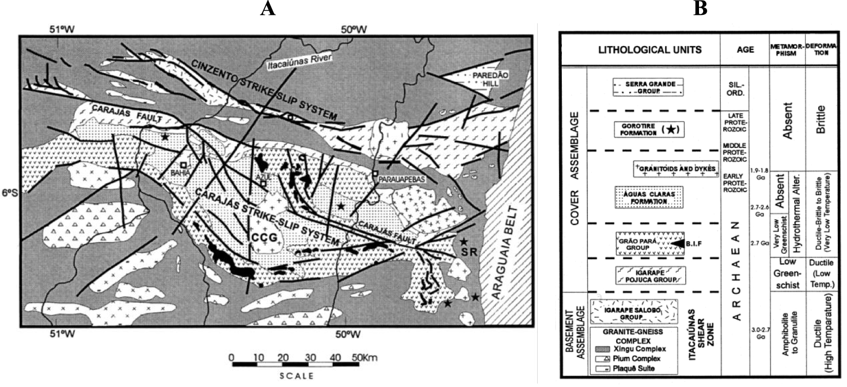
(A) Simplified geological map of the Carajas region. (SR = Serra do Rabo region; CCG = central Carajas granite). (B) Tectonostratigraphic description of the Carajas region (BIF = banded ironstone formation) [Holdsworth and Pinheiro 2000].

For this study, iron and aluminum oxide grades are used as a hard conditional data set due to the inequality constraint in their bivariate relationship. The data set consists of 608 sample points with iron and aluminum oxide grades measured in a homotopic sampling pattern, which means that both variables share the exact locations [Wackernagel 2003]. This is demonstrated in Figure 4 with location maps of iron and aluminum oxide grades. The southern part of the deposit is highly concentrated with iron and has considerably low aluminum oxide content, whereas the northern part has both low- and high-grade samples of iron and aluminum oxide.

Figure 4.
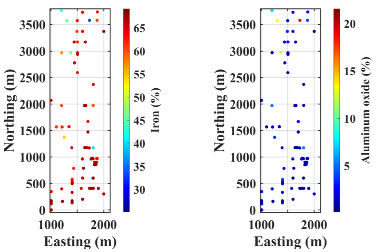
Location map of homotopic case study with two continuous variables: iron (left) and aluminum oxide (right).

3.2. Exploratory data analysis

According to visual inspection of location maps, it can be stated that there is a preferential sampling strategy. The sampling pattern is clustered in the area with high iron and low aluminum oxide grades; thus, the global equally weighted statistics of iron and aluminum oxide is biased. To alleviate this problem, a cell-declustering methodology [David 1977; Deutsch 1989] is implemented to eliminate the effect of clustering in the sampling pattern. After checking different possible declustered cell sizes, a 335 m × 770 m × 167.5 m cell dimension is selected as the most appropriate one. The declustered statistical parameters are shown in Table 1.

Statistical parameter	Iron (%)	Aluminum oxide (%)
Minimum	25.10	0.10
Maximum	69.17	32.10
Mean	63.07	2.27
Standard deviation	8.19	4.66
Coefficient of variation	0.13	2.05

Figure 5 shows grade distributions of iron and aluminum oxide in the histogram plots and bivariate distribution as a scatter plot. The majority of iron samples are higher than 65%, while most aluminum oxide grades are lower than 4%, with a strong negative correlation coefficient of −0.81. The histograms also show that these two variables possess two completely different distributions with positive and negative skewness (Figure 5A). Figure 5B demonstrates that most samples are disseminated in 60–70% iron content and 0–5% aluminum oxide content, where they show a clear inequality constraint in the bivariate relationship. The blue dashed line in Figure 5B represents this inequality constraint, which was obtained using Huber loss [Huber 1964] shifted upwards to identify the minimum support line [Madani and Abulkhair 2020]. Obtained coefficients of this line are with the slope w = −0.89 and intercept b = 62, thus an inequation is characterized as follows:

{Al}_{2} O_{3} ⩽ - 0.89 Fe + 62

(9)

Traditional cosimulation approaches are not able to reproduce such bivariate relationships. Battalgazy and Madani [2019] applied different stochastic geostatistical algorithms on the same data set by projection pursuit multivariate transform (PPMT) [Barnett et al. 2014, 2016], and turning bands simulation and cosimulation (TBSIM and TBCOSIM) [Matheron 1973; Lantuéjoul 1994; Emery and Lantuéjoul 2006; Emery 2008]. They showed that although PPMT can reproduce the correlation coefficient, unlike TBSIM and TBCOSIM, it could not reproduce the inequality constraint in the bivariate relationship. Madani and Abulkhair [2020] also verified that PPMT fails to reproduce such inequality constraint once they tested this on another data set. In this study, we aim to model the iron and aluminum oxide contents in this deposit by the proposed approach to examine which searching strategy is optimum honoring the inequality constraint in bivariate relationship.

Figure 5.
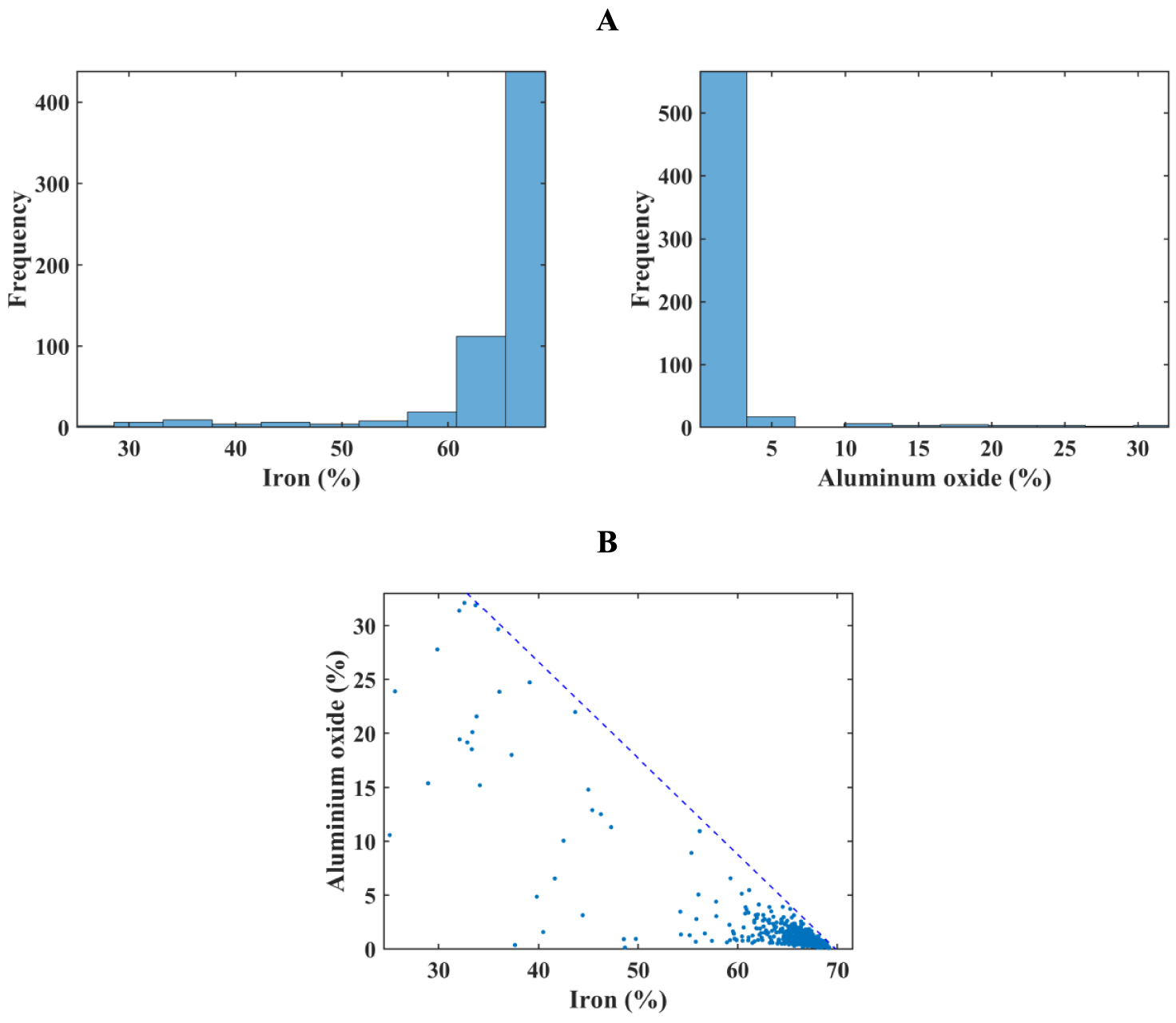
(A) Histogram plots of iron and aluminum oxide; and (B) scatterplot between variables. The minimum support line (blue dashed) is an inequation.

3.3. Variogram modeling

In order to perform hierarchical sequential Gaussian cosimulation, both variables ( $Z_{1}$ and Z₂) must be transformed to normal scores (Y₁ and Y₂) taking into account the declustering weights [Deutsch and Journel 1992]. The proposed hierarchical cosimulation algorithm is based on the multivariate Gaussianity assumption. Indeed, univariate Gaussian distribution and strong correlation do not mean that the multivariate distribution is Gaussian as well. The collocated scatter plot of the normal score transforms of both variables is presented as a check for bivariate Gaussianity. Figure 6A shows that both variables transformed to normal scores have univariate Gaussian distributions. The correlation between them is −0.71 and the shape of correlation is elliptical, meaning that bivariate Gaussianity can be reasonably assumed. A displaced bivariate Gaussianity check is implemented by producing lagged scatter plots for each transformed variable. At a specific distance, the points must be disseminated along with the elliptical shape [Rivoirard 1994]. Using a 15 m lag and 50% lag tolerance for lagged scatter plot, the bivariate distribution in the case of iron and aluminum oxide (Figure 6B) is also close to an elliptical shape. It can be concluded that the multi-Gaussianity assumption is reasonable and the proposed algorithm can be employed.

Figure 6.
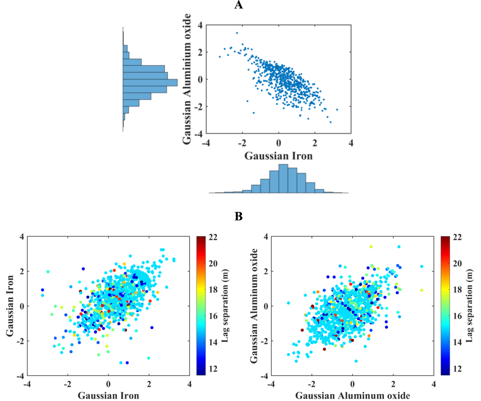
(A) Scatter plot between normal scores of iron and aluminum oxide accompanying their marginal distributions; (B) lagged scatter plots of normal scores of iron and aluminum oxide.

Next, the anisotropy is detected on the original data set before the transformation. As a result, three directions are identified: horizontal along the azimuth of 0° (north) as maximum continuity, horizontal along the azimuth of 90° (east) as medium continuity, and vertical as minimum continuity. Experimental direct- and cross-variograms required for the hierarchical cosimulation are calculated in these particular directions. Theoretical variograms are then fitted manually, and a two-structured linear model of coregionalization of iron (Fe) and aluminum oxide (Al₂O₃) is derived as in (Figure 7):

\begin{matrix} (\begin{matrix} 𝛾_{Fe} & 𝛾_{Fe ∕ {Al}_{2} O_{3}} \\ 𝛾_{{Al}_{2} O_{3} ∕ Fe} & 𝛾_{{Al}_{2} O_{3}} \end{matrix}) = (\begin{matrix} 0.45 & - 0.30 \\ - 0.30 & 0.45 \end{matrix}) Sph (100 m, 60 m, 30 m) \\ + (\begin{matrix} 0.40 & - 0.40 \\ - 0.40 & 0.47 \end{matrix}) Sph (500 m, 300 m, 150 m) \end{matrix}

(10)

Figure 7.
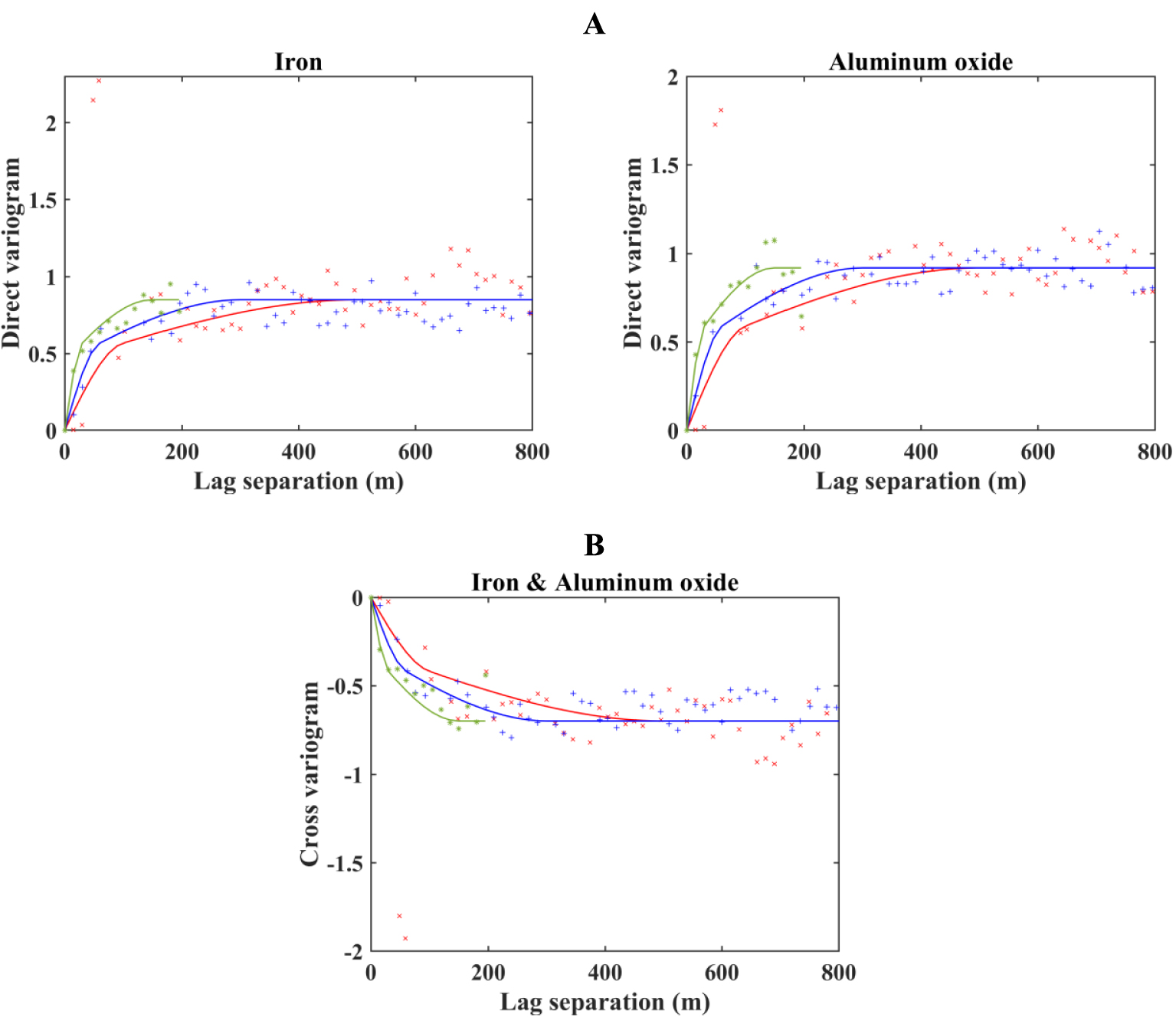
(A) Direct and (B) cross-variograms of the normal scores of iron and aluminum oxide, where experimental variograms are indicated as point crosses and theoretical variograms with solid lines. Red: horizontal direction with the azimuth of 0°; blue: horizontal direction with the azimuth of 90°; and green: vertical direction.

3.4. Simulation results

Before conducting the hierarchical cosimulation, primary and secondary variables must be selected. Investigation of omnidirectional variogram of iron and aluminum oxide demonstrated that iron has a better spatial continuity that makes it worth being selected as the primary variable. Another reason for selecting the iron as the primary variable is that the iron in this deposit plays an important role and is indicated as the main variable of interest. However, aluminum oxide is deemed as a deleterious element, meaning that its influence on long- and short-term mine planning is inevitable.

The hierarchical cosimulation proposed in the case of two cross-correlated variables can be carried out in two consecutive steps; first to simulate the primary variable in the entire region, and second to simulate the secondary variable conditional to the first run of the simulation. Therefore, in this study, two searching strategy combinations are examined:

Single & Single (S&S): Implementing the first step of cosimulation by single and second step by single searching strategies, respectively.
Multiple & Multiple (M&M): Implementing the first step of cosimulation by multiple and second step by multiple searching strategies, respectively.

Integration of these moving neighborhood strategies was assessed in the proposed algorithm (i.e., taking into account an inequality constraint) and compared with the conventional hierarchical cosimulation (i.e., without inequality constraint). The latter does not consider the inequation restriction in contrast to the former, where an inverse transform sampling is applied to reproduce the identified inequality constraint. The abbreviation “IC” indicates the proposed algorithm all over the paper because it is generated to reproduce inequality constraints between coregionalized variables. Therefore, the conventional approach is identified by (A) Single & Single search (S&S) and (B) Multiple & Multiple search (M&M); and the proposed approach is identified by (C) Single & Single search (S&S IC) and (D) Multiple & Multiple search (M&M IC). For this purpose, one plane of a grid with dimensions of 15 m × 15 m × 15 m is considered for comparison. Figure 8 demonstrates one realization from each search strategy integrated into conventional (A and B) and proposed (C and D) hierarchical cosimulation algorithms.

Figure 8.
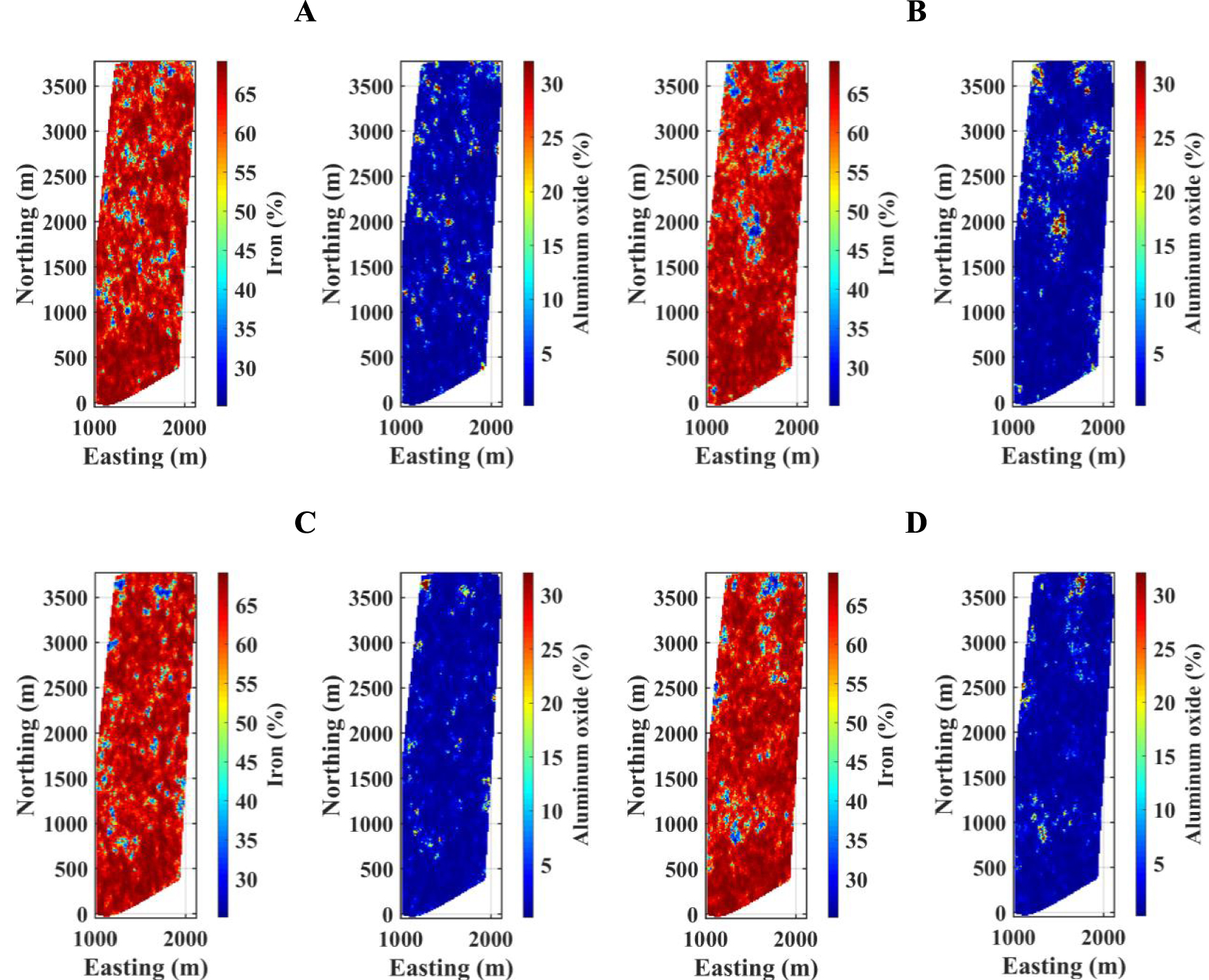
Realization maps of iron and aluminum oxide obtained from conventional hierarchical cosimulation with (A) Single & Single search, (B) Multiple & Multiple search; from proposed hierarchical cosimulation with, (C) Single & Single search, and (D) Multiple & Multiple search.

3.5. Reproduction of global statistical parameters

In order to examine the proposed algorithm, validation of geostatistical algorithms mainly consists of a reproduction of first-order statistics or histogram reproduction, and second-order statistics or variogram reproduction. First-order statistics includes global statistical parameters such as mean, standard deviation, coefficient of variation, and correlation coefficient. To validate the reproduction of global statistical parameters, original declustered means, standard deviations, and correlation coefficients are compared to average statistical parameters over 100 realizations (Table 2) from both hierarchical cosimulation approaches. In addition to the four cases (i.e., S&S, M&M, S&S IC, M&M IC), two other alternatives are also taken into account for the validation part. These two cases are (1) Single & Multicollocated IC search (S&MC IC), and (2) Multiple & Multicollocated IC search (M&MC IC), for which they are compatible with the approaches proposed in Madani and Abulkhair [2020], where the second searching strategy follow a multicollocated neighborhood.

As can be seen, all the searching strategies more or less are the same and capable of reproducing the declustered original statistical parameters of iron (Table 2). Nevertheless, global statistical parameters of aluminum oxide are considerably underestimated. In this regard, conventional cosimulation methodology underestimates the original mean of aluminum oxide by 9–17%, while the proposed methodology shows a deviation of 31–36%. Similarly, standard deviations are underestimated by 10–20% using the conventional methodology and by 37–45% using the proposed methodology. Therefore, it can be observed that there is a severe underestimation of global statistical parameters of the secondary variable when using the proposed methodology. This issue has not yet been resolved by the authors. However, it is worth mentioning that the implementation of an M&M strategy demonstrated better reproduction of global statistics for both conventional and proposed cosimulation algorithms.

Figure 9.
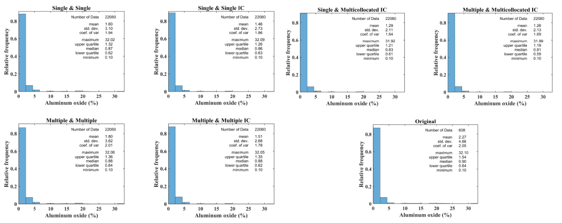
Histogram reproduction of aluminum oxide simulated by (A) conventional and proposed hierarchical cosimulation using single and multiple search strategies, (B) hierarchical cosimulation using single and multiple searching strategies in the first simulation and multicollocated in the second searching strategy.

Statistical parameter	Original	S&S	M&M	S&S IC	M&M IC	S&MC IC	M&MC IC
Correlation coefficient	−0.81	−0.60	−0.62	−0.67	−0.68	−0.66	−0.67
% vs original	—	74%	77%	83%	84%	81%	83%
Iron (%)
Mean	63.07	63.74	63.48	63.74	63.48	63.74	63.48
% vs original	—	101%	101%	101%	101%	101%	101%
Standard deviation	8.19	7.04	7.48	7.04	7.48	7.04	7.48
% vs original	—	86%	91%	86%	91%	86%	91%
Aluminum oxide (%)
Mean	2.27	1.88	2.07	1.48	1.57	1.45	1.54
% vs original	—	83%	91%	65%	69%	64%	68%
Standard deviation	4.66	3.73	4.20	2.65	2.94	2.55	2.82
% vs original	—	80%	90%	57%	63%	55%	61%

Figure 9 shows the reproduction of the univariate marginal distribution of the secondary variable, aluminum oxide, in the first realization of each simulation. The objective of histogram validation is to analyze how using the proposed methodology affects the reproduction of the shape of the marginal distribution. In this case, all the algorithms are able to reproduce the shape of aluminum oxide’s histograms, although the conventional cosimulation is better in the reproduction of basis statistical parameters.

The main objective of the proposed hierarchical cosimulation with inequality constraint is to reproduce the original declustered data set’s bivariate relationship. Figure 10A, B demonstrates scatter plots between two simulated variables in the first realization and compares them to the original bivariate relationship. Conventional hierarchical cosimulation fails to reproduce the original scatter plot considering the bivariate relationship and its results have some unrealistic points with high grades of both iron and aluminum oxide above the inequation line. However, there is no significant difference between S&S and M&M searching strategies. Besides, the results produced by the cosimulation algorithm using a multicollocated searching strategy as in the second search (Figure 10C) show similar bivariate characteristics to the scatter plots of S&S IC and M&M IC. This type of validation can only confirm the reproduction of the underlying inequality constraint, while the visual inspection of scatter plots may not significantly contribute to identifying the best strategy among the searching strategies with IC method.

Figure 10.
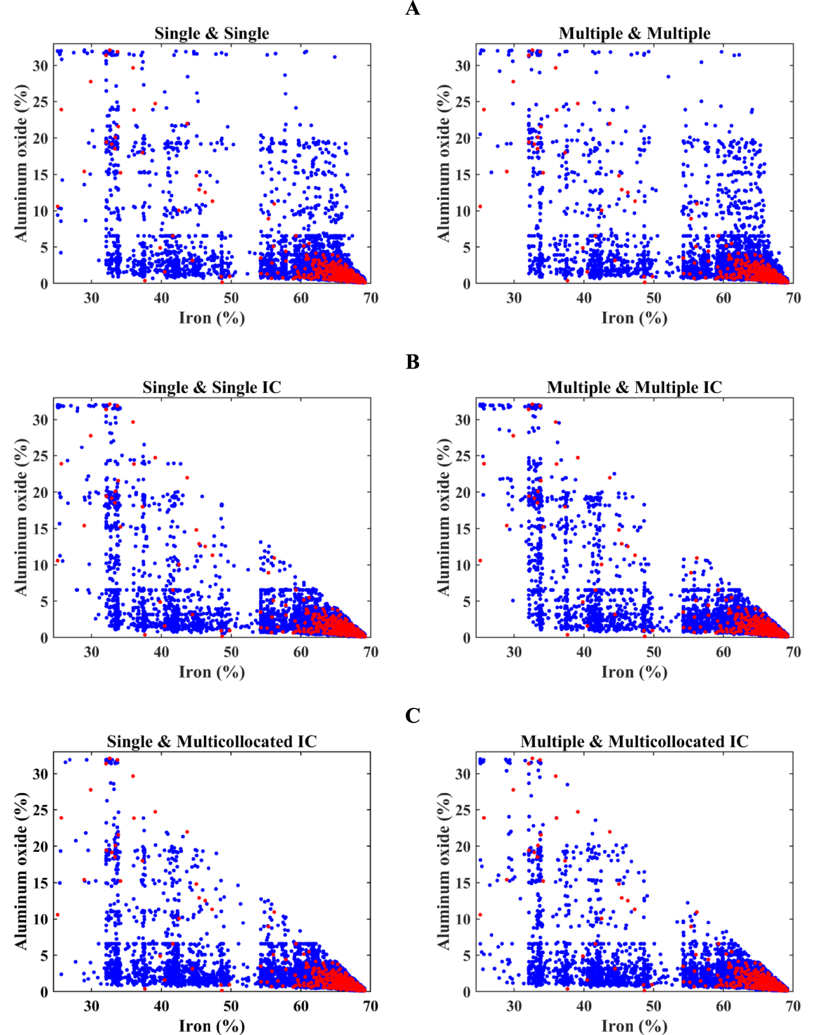
Reproduction of bivariate relationship between iron and aluminum oxide simulated by (A) conventional and (B) proposed hierarchical cosimulation using single and multiple search strategies, (C) hierarchical cosimulation using single and multiple searching strategies in the first simulation and multicollocated in the second. Blue: scatter plot of simulated values for realization #1; and red: scatter plot of original values.

Figure 11.
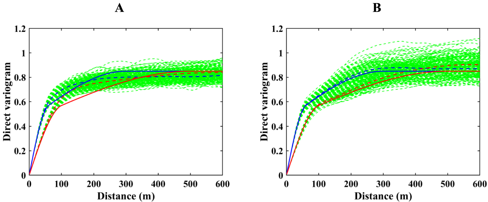
Direct variograms of iron simulated by hierarchical cosimulation using (A) single and (B) multiple search strategies. Green: variograms of 100 realizations; red: north direction; blue: east direction; dashed: average over realizations; and solid: theoretical. (Direct variograms are standardized to prevent numerical instabilities.)

3.6. Reproduction of local statistical parameters

Previous statistical validations focus on global statistical parameters, but it has less importance compared to local statistics. The simplest way of local statistics validation is variogram reproduction. The proposed and conventional cosimulation algorithms are identical in simulating the iron, since this is the first run in hierarchical paradigm. The only difference is related to the searching neighborhood used in these algorithms. Figure 11 shows the reproduction of direct variograms of iron over the simulated results to compare such a difference. As can be seen, multiple searching strategy produces better results compared to the case when the neighborhood follows a single searching strategy.

Comparison between two searching strategies integrated into conventional and proposed hierarchical cosimulation techniques using direct variogram reproduction of aluminum oxide in maximum and minimum horizontal directions is shown in Figure 12A, B. Although the M&M strategy produces more fluctuations, its average variograms resemble the theoretical model. On the other hand, the S&S strategy can only reproduce the first structure but ultimately fails to reproduce the second structure’s desired sill and range. Figure 12C shows direct variogram validation of aluminum oxide simulated by the algorithm, where a multicollocated searching strategy is used in the second simulation run instead of a heterotopic one. It can be observed that choosing an appropriate neighborhood configuration in the first simulation can affect the overall quality of realizations for the second variable. This means that using a single search in the first simulation always deteriorates the reproduction of the second variable’s variogram ranges as well. On the other hand, a combination of M&MC searching strategies shows better variogram reproduction, particularly when both searching strategies are M&M.

Figure 12.
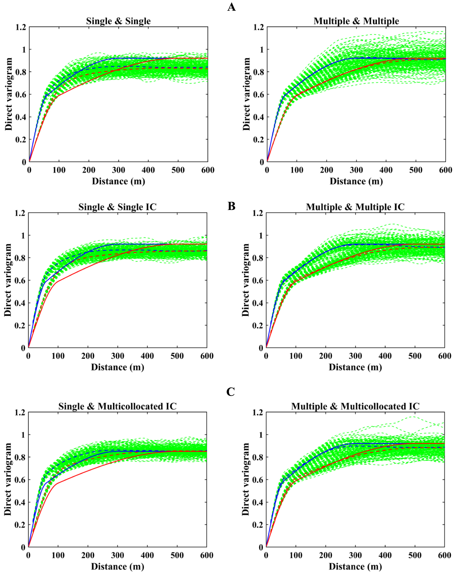
Direct variograms of aluminum oxide simulated by (A) conventional, (B) proposed hierarchical cosimulation using single and multiple search strategies, and (C) proposed hierarchical cosimulation using single and multiple searching strategies in the first simulation and multicollocated in the second. Green: variograms of 100 realizations; red: north direction; blue: east direction; dashed: average over realizations; and solid: theoretical. (Direct variograms are standardized to prevent numerical instabilities.)

Figure 13.
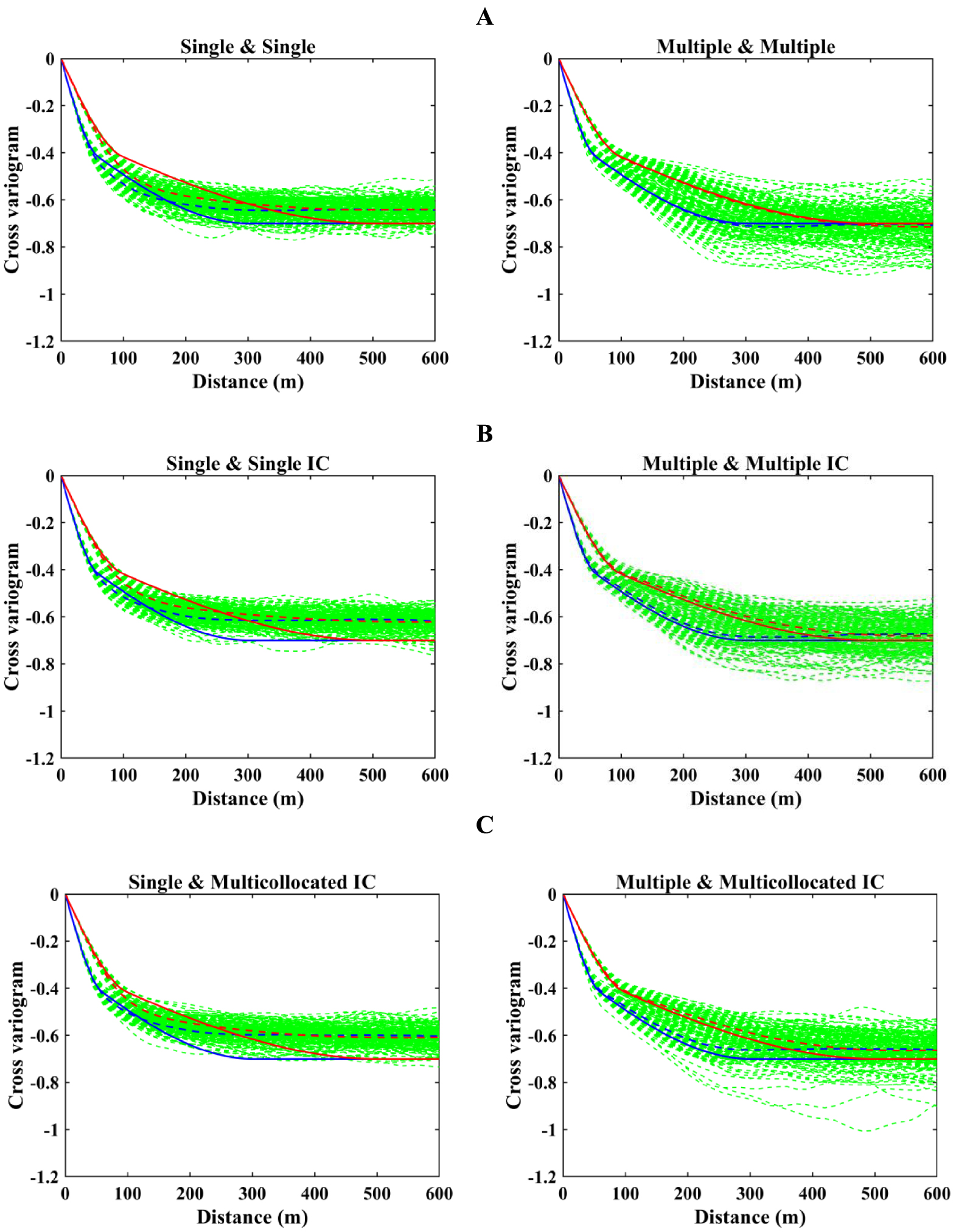
Cross-variograms between iron and aluminum oxide simulated by (A) conventional, (B) proposed hierarchical cosimulation using single and multiple search strategies, and (C) proposed hierarchical cosimulation using single and multiple searching strategies in the first simulation and multicollocated in the second. Green: variograms of 100 realizations; red: north direction; blue: east direction; dashed: average over realizations; and solid: theoretical.

Another essential objective of hierarchical cosimulation is the reproduction of cross-correlation structure between variables, and one way to assess this feature is to examine the reproduction of cross-variograms. Figure 13A, B shows that the S&S strategy cannot reproduce the theoretical shape of cross-variogram, while the M&M strategy perfectly meets the theoretical model of cross-variogram. Moreover, conventional and proposed approaches have a very insignificant difference in terms of variogram reproduction, which shows the effectiveness of the hierarchical cosimulation algorithm in the case of M&M whether the inequality constraint is considered or not. In order to investigate how heterotopic searching strategies perform in combination with multicollocated configuration, this part validates the reproduction of cross-variograms using S&MC IC and M&MC IC strategies as well (Figure 13C). Unlike single search, multiple searching strategy is able to reproduce the second structure’s ranges. However, M&M IC show better results in cross-variogram reproduction even when it is compared with M&MC IC.

4. Conclusion

A methodology based on a hierarchical sequential Gaussian cosimulation is proposed in this study integrated with an inverse transform sampling technique to simulate the values of the secondary variable conditionally to the primary variable, where both show inequality constraint. In this technique, an inequation can be imposed so that the simulated values fall below the preidentified linear function derived by an inequation. This sampling technique ensures the higher speed of the algorithm compared to an acceptance–rejection technique. A heterotopic SCK is also embedded into the process of cosimulation with two alternatives of search strategies for establishing a moving neighborhood for both steps of this algorithm: Single & Multiple searching strategies. The comparison of results with conventional hierarchical cosimulation is made using a real case study from an iron deposit. It showed that the proposed algorithm is able to reproduce the bivariate inequality constraint between two underlying cross-correlated variables. The comparison between the Multiple searching strategy and the Single searching strategy also revealed that the former outperforms the latter in reproducing statistical parameters. Although histogram and variogram validations showed promising results for a M&M searching strategy in all algorithms; however, the reproduction of mean and standard deviation of the secondary variable in the proposed algorithm is questionable. For this, integration of an inverse transform sampling likely resulted in the reproduction of aluminum oxide’s mean value that is being underestimated by around 31–36%, compared to an underestimation of 9–17% in the conventional algorithm. Likewise, standard deviation results showed an underestimation of 37–45%.

Effects of heterotopic searching strategies are also investigated in combination with multicollocated search integrated into the second simulation of the proposed algorithm. Histogram, scatter plot, and variogram validations are presented for S&MC IC and M&MC IC strategies. Results of variogram validation demonstrated that a single searching strategy poorly reproduces the spatial continuity of iron. Poor reproduction of the primary variable negatively affects the simulation of the secondary variable either. Overall, using a multiple searching strategy in both simulations of a hierarchical cosimulation process is proven to be more suitable for this particular iron deposit. The findings of this research are also compatible with Madani and Emery [2019] results, where they argued that single search is less precise than multiple searching strategies in establishing the cokriging systems.

However, there is still more work to be done with the proposed algorithm. For instance, a cosimulation can be adopted to the hierarchical algorithm where geological domains regulate the cross-correlated variables with inequality constraints. In the case of a soft boundary, this algorithm can be updated to a joint simulation paradigm, where a Gibbs sampler with multivariate Gaussian distribution is required to be adjusted. Another improvement can be related to the involvement of more continuous variables in the algorithm. The proposed algorithm also needs further improvement in order to better reproduce basic statistics when imposing inequality constraints.

Author contributions

SA implemented the case study, contributed to its analysis and interpretation, assisted in final algorithm design, wrote and revised the paper. NM developed the original idea and background methodology, algorithm design and helped to revise the final version of the manuscript.

Competing interests

The authors declare no competing interests.

Acknowledgments

The authors are grateful to Nazarbayev University for funding this work via “Faculty Development Competitive Research Grants for 2018–2020 under Contract No. 090118FD5336”. The authors also thank the Geovariances Company for providing the iron data set. We are also thankful to the Editorial team and anonymous reviewer for their valuable comments, which helped to improve the paper and the quality of results.

Bibliographie

[Abildin et al., 2019] Y. Abildin; N. Madani; E. Topal A hybrid approach for joint simulation of geometallurgical variables with inequality constraint, Minerals, Volume 9 (2019) no. 1, 24 | DOI

[Adeli et al., 2018] A. Adeli; X. Emery; P. Dowd Geological modelling and validation of geological interpretations via simulation and classification of quantitative covariates, Minerals, Volume 8 (2018) no. 1, 7 | DOI

[Almeida and Journel, 1994] A. S. Almeida; A. G. Journel Joint simulation of multiple variables with a Markov-type coregionalization model, Math. Geol., Volume 26 (1994), pp. 565-588 | DOI

[Arcari Bassani et al., 2018] M. A. Arcari Bassani; J. Costa; C. V. Deutsch Multivariate geostatistical simulation with sum and fraction constraints, Appl. Earth Sci., Volume 127 (2018) no. 3, pp. 83-93

[Barnett et al., 2014] R. M. Barnett; J. G. Manchuk; C. V. Deutsch Projection pursuit multivariate transform, Math. Geosci., Volume 46 (2014), pp. 337-359 | DOI | MR | Zbl

[Barnett et al., 2016] R. M. Barnett; J. G. Manchuk; C. V. Deutsch The projection-pursuit multivariate transform for improved continuous variable modeling, Soc. Pet. Eng., Volume 21 (2016) no. 6, pp. 2010-2026

[Battalgazy and Madani, 2019] N. Battalgazy; N. Madani Categorization of mineral resources based on different geostatistical simulation algorithms: A case study from an iron ore deposit, Nat. Resour. Res., Volume 28 (2019), pp. 1329-1351 | DOI

[Beisiegel et al., 2018] V. R. Beisiegel; A. L. Bemardelli; N. F. Drummond; A. W. Ruff; J. W. Tremaine Geologia e recursos minerais da Serra dos Carajás, Rev. Bras. Geociênc., Volume 3 (2018) no. 4, pp. 215-242

[Burkardt, 2014] J. Burkardt The Truncated Normal Distribution, 2014 https://people.sc.fsu.edu/~jburkardt/presentations/truncated_normal.pdf (Department of Scientific Computing Website, Florida State University)

[BVP, 2011] BVP Lithostructural and lithogeomechanical mapping of the N4E mine (2011) (BVP Engenharia Internal Report) (Technical report)

[Chilès and Delfiner, 2012] J. P. Chilès; P. Delfiner Geostatistics: Modeling Spatial Uncertainty, Wiley, New York, 2012 | Zbl

[David, 1977] M. David Geostatistical Ore Reserve Estimation, Elsevier, New York, 1977

[Desbarats and Dimitrakopoulos, 2000] A. J. Desbarats; R. Dimitrakopoulos Geostatistical simulation of regionalized pore-size distributions using min/max autocorrelation factors, Math. Geol., Volume 32 (2000), pp. 919-942 | DOI

[Deutsch and Journel, 1992] C. V. Deutsch; A. G. Journel GSLIB: Geostatistical Software Library and Users Guide, Oxford University Press, New York, 1992

[Deutsch, 1989] C. V. Deutsch DECLUS: a fortran 77 program for determining optimum spatial declustering weights, Comput. Geosci., Volume 15 (1989) no. 3, pp. 325-332 | DOI

[Devroye, 1986] L. Devroye Non-Uniform Random Variate Generation, Springer, New York, 1986 | DOI | Zbl

[Emery and Lantuéjoul, 2006] X. Emery; C. Lantuéjoul TBSIM: A computer program for conditional simulation of three-dimensional Gaussian random fields via the turning bands method, Comput. Geosci., Volume 32 (2006) no. 10, pp. 1615-1628 | DOI

[Emery, 2008] X. Emery A turning bands program for conditional co-simulation of cross-correlated Gaussian random fields, Comput. Geosci., Volume 34 (2008) no. 12, pp. 1850-1862 | DOI

[Goovaerts, 1997] P. Goovaerts Geostatistics for Natural Resource Evaluation, Oxford University Press, New York, 1997

[Holdsworth and Pinheiro, 2000] R. E. Holdsworth; R. V. L. Pinheiro The anatomy of shallow-crustal transpressional structures: insights from Archean Carajás fault zone, Amazon, Brazil, J. Struct. Geol., Volume 22 (2000), pp. 1105-1123 | DOI

[Huber, 1964] P. J. Huber Robust estimation of a location parameter, Ann. Math. Stat., Volume 35 (1964) no. 1, pp. 73-101 | DOI | MR | Zbl

[Lantuéjoul, 1994] C. Lantuéjoul Non conditional simulation of stationary isotropic multigaussian random functions, Geostatistical Simulations (M. Armstrong; P. A. Dowd, eds.), Springer, Dordrecht, 1994, pp. 147-177 | DOI

[Leuangthong and Deutsch, 2003] O. Leuangthong; C. V. Deutsch Stepwise conditional transformation for simulation of multiple variables, Math. Geol., Volume 35 (2003), pp. 155-173 | DOI | Zbl

[Madani and Abulkhair, 2020] N. Madani; S. Abulkhair A hierarchical cosimulation algorithm integrated with an acceptance–rejection method for the geostatistical modeling of variables with inequality constraints, Stoch. Environ. Res. Risk Assess., Volume 34 (2020) no. 10, pp. 1559-1589 | DOI

[Madani and Emery, 2019] N. Madani; X. Emery A comparison of search strategies to design the cokriging neighborhood for predicting coregionalized variables, Stoch. Environ. Res. Risk Assess., Volume 33 (2019), pp. 183-199 | DOI

[Matheron, 1973] G. Matheron The intrinsic random functions and their applications, Adv. Appl. Probab., Volume 5 (1973) no. 3, pp. 439-468 | DOI | MR | Zbl

[Meireles et al., 1984] E. M. Meireles; W. K. Hirata; A. F. Amaral; C. A. Medeiros Filho; W. A. Gato Geologia das folhas Carajás e Rio Verde, Província Mineral de Carajás, Estado do Pará, 33 Congresso Brasileiro de Geologia, Sociedade Brasileira de Geologia, Rio de Janeiro, Brazil, 1984, pp. 2164-2170

[Mery et al., 2017] N. Mery; X. Emery; A. Cáceres; D. Ribeiro; E. Cunha Geostatistical modeling of the geological uncertainty in an iron ore deposit, Ore Geol. Rev., Volume 88 (2017), pp. 336-351 | DOI

[Paradella et al., 2015] W. R. Paradella; A. Ferretti; J. C. Mura; D. Colombo; F. F. Gama; A. Tamburini; A. R. Santos; F. Novali; M. Galo; P. O. Camargo; A. Q. Silva; G. G. Silva; A. Silva; L. L. Gomes Mapping surface deformation in open pit iron mines of Carajás Province (Amazon Region) using an integrated SAR analysis, Eng. Geol., Volume 193 (2015), pp. 61-78 | DOI

[Pawlowsky-Glahn and Egozcue, 2006] V. Pawlowsky-Glahn; J. J. Egozcue Compositional data and their analysis: An introduction, Geol. Soc. Lond. Spec. Publ., Volume 264 (2006) no. 1, pp. 1-10 | DOI | Zbl

[Pawlowsky-Glahn and Olea, 2004] V. Pawlowsky-Glahn; R. A. Olea Geostatistical Analysis of Compositional Data, Oxford University Press, Oxford, 2004 | Zbl

[Pyrcz and Deutsch, 2014] M. J. Pyrcz; C. V. Deutsch Geostatistical Reservoir Modeling, Oxford University Press, New York, 2014

[Rivoirard, 1994] J. Rivoirard Introduction to Disjunctive Kriging and Nonlinear Geostatistics, Oxford University Press, Oxford, 1994

[Rossi and Deutsch, 2014] M. E. Rossi; C. V. Deutsch Mineral Resource Estimation, Springer, Berlin, 2014

[Tran, 1994] T. T. Tran Improving variogram reproduction on dense simulation grids, Comput. Geosci., Volume 20 (1994) no. 7-8, pp. 1161-1168 | DOI

[van den Boogaart et al., 2017] K. G. van den Boogaart; U. Mueller; R. Tolosana-Delgado An affine equivariant multivariate normal score transform for compositional data, Math. Geosci., Volume 49 (2017), pp. 231-251 | DOI | MR | Zbl

[Vargas-Guzmán and Dimitrakopoulos, 2003] J. A. Vargas-Guzmán; R. Dimitrakopoulos Successive nonparametric estimation of conditional distributions, Math. Geol., Volume 35 (2003), pp. 39-52 | DOI | MR | Zbl

[Verly, 1993] G. W. Verly Sequential Gaussian cosimulation: A simulation method integrating several types of information, Geostatistics Tróia’92. Quantitative Geology and Geostatistics (A. Soares, ed.), Volume 5, Springer, Dordrecht, 1993, pp. 543-554 | DOI

[Wackernagel, 2003] H. Wackernagel Multivariate Geostatistics, Springer, Berlin, 2003 | DOI | Zbl