The improvement of the Morlet wavelet for multi-period analysis of climate data

Hua Yi; Hong Shu

doi:10.1016/j.crte.2012.09.007

External geophysics, climate

The improvement of the Morlet wavelet for multi-period analysis of climate data
[Perfectionnement de la méthode de l’ondelette de Morlet pour l’analyse multipériodes des données climatiques]

Présenté par : Michel Petit

Hua Yi ^1,² ; Hong Shu ³

¹ Department of Mathematics, Jinggangshan University, Ji’an, Jiangxi Province, 343009, People's Republic of China
² School of Mathematics and Statistics, Wuhan University, Wuhan, People's Republic of China
³ The State Key Laboratory for Information Engineering in Surveying, Mapping and Remote Sensing, Wuhan University, Wuhan, People's Republic of China

Comptes Rendus. Géoscience, Volume 344 (2012) no. 10, pp. 483-497.

Résumés

Anglais
Français

The multi-level dynamics of an atmosphere system exhibits temporal structures in different types of climate data. This article addresses two issues in multi-period analysis of climate data. Firstly, the advantages of the modified Morlet wavelet transform (MMWT) for analyzing multi-period structure of time series over Morlet wavelet transform (MWT) are emphasized. Secondly, the multi-period issues of temperature data are studied with MMWT through four steps: the four dominant periods of 60 year temperature data are determined with the wavelet variance; by analyzing the real part of MMWT, the warm and cold stages of the temperature data at different scales are determined, and the time intervals of the warm and cold interchange are singled out; the amplitude of each periodic component is quantitatively characterized by the amplitude of wavelet coefficients; the most intensive oscillation time intervals are computed by the squared modulus of the MMWT (MMPS).

La dynamique multiniveaux d’un système atmosphérique indique des structures temporelles dans différents types de données climatiques. Cet article concerne deux aspects relatifs à l’analyse multipériodes des données climatiques. D’abord, les avantages de la transformée modifiée d’ondelette de Morlet (MMWT) pour analyser la structure multipériodes des séries temporelles sur transformée d’ondelette de Morlet (MWT) sont mis en évidence. Ensuite, les aspects multipériodes des données sur la température sont étudiés par la méthode MMWT en quatre étapes : les quatre périodes dominantes sur les mesures de température annuelle sont déterminées par la variance d’ondelette ; par l’analyse de la part réelle de MMWT, les phases de température chaudes et froides à différentes échelles sont déterminées, et les intervalles de temps dans l’échange chaud–froid distingués ; l’amplitude de chaque composant périodique est caractérisée par l’amplitude des coefficients d’ondelette ; les intervalles de temps d’oscillation les plus intenses sont calculés par le module carré de MMWT (MMPS).

Métadonnées

Reçu le : 2011-12-06
Accepté le : 2012-09-28
Publié le : 2012-10-01

DOI : 10.1016/j.crte.2012.09.007

Keywords: Morlet wavelet, Gaussian window, Scale-to-frequency formula, Wavelet variance, Multi-period
Mot clés : Ondelette de Morlet, Fenêtre gaussienne, Formule échelle-fréquence, Variance d’ondelette, Multipériodes

Affiliations des auteurs :

Hua Yi ^{1, 2} ; Hong Shu ³

¹ Department of Mathematics, Jinggangshan University, Ji’an, Jiangxi Province, 343009, People's Republic of China
² School of Mathematics and Statistics, Wuhan University, Wuhan, People's Republic of China
³ The State Key Laboratory for Information Engineering in Surveying, Mapping and Remote Sensing, Wuhan University, Wuhan, People's Republic of China

@article{CRGEOS_2012__344_10_483_0,
     author = {Hua Yi and Hong Shu},
     title = {The improvement of the {Morlet} wavelet for multi-period analysis of climate data},
     journal = {Comptes Rendus. G\'eoscience},
     pages = {483--497},
     publisher = {Elsevier},
     volume = {344},
     number = {10},
     year = {2012},
     doi = {10.1016/j.crte.2012.09.007},
     language = {en},
}

TY  - JOUR
AU  - Hua Yi
AU  - Hong Shu
TI  - The improvement of the Morlet wavelet for multi-period analysis of climate data
JO  - Comptes Rendus. Géoscience
PY  - 2012
SP  - 483
EP  - 497
VL  - 344
IS  - 10
PB  - Elsevier
DO  - 10.1016/j.crte.2012.09.007
LA  - en
ID  - CRGEOS_2012__344_10_483_0
ER  -

%0 Journal Article
%A Hua Yi
%A Hong Shu
%T The improvement of the Morlet wavelet for multi-period analysis of climate data
%J Comptes Rendus. Géoscience
%D 2012
%P 483-497
%V 344
%N 10
%I Elsevier
%R 10.1016/j.crte.2012.09.007
%G en
%F CRGEOS_2012__344_10_483_0

Hua Yi; Hong Shu. The improvement of the Morlet wavelet for multi-period analysis of climate data. Comptes Rendus. Géoscience, Volume 344 (2012) no. 10, pp. 483-497. doi : 10.1016/j.crte.2012.09.007. https://comptes-rendus.academie-sciences.fr/geoscience/articles/10.1016/j.crte.2012.09.007/

Version originale du texte intégral

1 Introduction

The determination of multi-period structures of time series is an important part of meteorological data mining. Complex geographical phenomena are mostly the result of dynamic interaction at different scales and different times (location), and the strength of dynamic action may differ from one scale to another. A specific time (or space) and scale (or frequency) can characterize in detail the temporal and spatial structure of geographical phenomena. Moreover, the complexity of the local climate change may be aggravated by the interplay of global phenomena such as the widely studied sunspot number (Chattopadhyay and Chattopadhyay, 2012) and total ozone (Chattopadhyay et al., 2011). Therefore, the effective methods for determination of multi-period structures of time series are useful.

Wavelet analysis is one such powerful tool well-suited to study multiscale, nonstationary processes occurring over finite spatial and temporal domains. During the 1990s, it has been successfully used in signal processing, such as image coding, compressing and edge detection. In the recent years, wavelet transform (WT) has found numerous applications in Geophysics. In 1993, Meyers et al. have studied the dispersion of Yanai waves and the relationship between the equivalent Fourier period and the wavelet scale for Morlet wavelets was derived (Meyers et al., 1993). Torrence and Compo (1998) have given a practical step-by-step guide to wavelet analysis, with examples taken from time series of the El Niño-Southern Oscillation (ENSO), and have written a program for computing the continuous wavelet transform (CWT) of time series (Torrence and Compo, 1998).

The Morlet wavelet is a periodic function enveloped by a Gaussian function. Therefore, the Morlet wavelet transform has been widely used to identify periodic oscillations of real-life signals (Issac et al., 2004; Labat, 2005; Labat et al., 2005; Werner, 2008). However, all of the aforementioned papers adopted WT with respect to the L₂ norm and this convention can be traced back to the pioneering work of Grossmann and Morlet (1984) about the wavelet.

On the other hand, to the best of our knowledge, the first application of WT w.r.t the L₁ norm was studied by Guillemain et al. (1991). Then, this sort of WT was used to explore the frequency and amplitude modulation laws by using the phase of the WT (Delprat et al., 1992; Saracco et al., 1991), and this method was also used to extract orbital frequencies for palaeomagnetic/palaeoclimate data (Saracco et al., 2009).

Considering the extensive use of WT with the two norms, more attention should be paid to the comparisons between the two methods. The work of Shyu and Sun (2002) states that conducting Morlet wavelet transform (corresponding to the L₂ norm) for signals with the same amplitude but different frequencies may produce the squared modulus of Morlet wavelet transform (MPS) with different amplitudes. In contrast to MWT and MPS, conducting the modified Morlet wavelet transform (MMWT, corresponding to the L₁ norm) for signals with the same amplitude, but different frequencies can get MMPS with the same amplitude. Then the results are demonstrated by Yi et al. (2010) under the condition that time parameter b is an arbitrary value while the results of Shyu and Sun (2002) are obtained by experiments under the condition that time parameter b is equal to 0. Furthermore, not only are the above results summarized in Yi et al. (2010), but also the quantitative characterizations between the signal amplitude, frequency and wavelet power spectrum are given.

The Morlet wavelet is obtained through the Gaussian window frequency modulation. So, we can introduce a shape parameter σ² to control the shape of the Gaussian window, and balance the time resolution and the frequency resolution (Mallat, 2009). In order to choose the optimal parameter σ², wavelet entropy is introduced, and the parameter σ², upon which the wavelet entropy obtains its minimum, is chosen as the ideal parameter (Lin and Qu, 2000). In this article, we have studied the properties of the Morlet wavelet with the shape parameter. Furthermore, by varying the shape parameter σ² and center frequency η defined in (1), the Morlet wavelets can be given a broad range of characteristics so that they can be fitted to practical data.

The results concerning the Morlet wavelet without shape parameter in Yi et al. (2010) are composed of two parts, one is that MMWT maintains the same amplitude between the original frequency component and the wavelet coefficients; therefore, the intensity of oscillation of periodic component of signal can be accurately characterized by the amplitude of the corresponding wavelet coefficients. On the contrary, the maximum of MPS is proportional to the squared amplitude of the frequency component, and is inversely proportional to the size of the frequency. In this article, we make a generalization of the results in Yi et al. (2010) by using the Morlet wavelet with the shape parameter. Furthermore, we can have a concise demonstration in this article by calculating integral in frequency domain instead of the integral in time domain in Yi et al. (2010).

Based on the theory of Yi et al. (2010), Yi and Fan (2010) gave an algorithm to distinguish the multi-period structure of 55 years of temperature data and Matlab generated data. In this article, the method of Yi et al. is improved. Furthermore, the theory based on the Morlet wavelet with shape parameter will make for a more complete theoretical foundation of this method.

This article focuses on the comparisons between MWT and MMWT, which will deepen our understanding of WT. To sum up, it is an advantage to use MMWT if we analyze the features of data because this analysis can focus all the attention to the characteristic of the data without concerning the inverse wavelet transform (IWT), while it is better to use WT w.r.t L₂ norm if IWT is concerned due to the orthonormal basis of L₂ space. In addition, we pay more attention to the quantitative description of data and the mother wavelet, which may not be much concerned, and may be a complement to those papers about the frequency and amplitude modulation laws by using the phase of the WT.

In other words, we think the main contribution of this article is described in Section 3, in which the advantage of MMWT is demonstrated when analyzing the characteristics of data. At the same time, Section 2 gives the necessary concept about the wavelet; Section 4 is just an experimentation in order to support the arguments of Section 3, in which the multi-period structure of temperature data for No. 50978 station of Heilongjiang, China is analyzed; Section 5 gives the conclusion of this article.

2 Morlet wavelet and wavelet transform

2.1 The Morlet wavelet with shape parameter

The Morlet wavelet consists of a sinusoidal wave modified by a Gaussian envelope, so it is given as (Mallat, 2009):

ψ (t) = C e^{\frac{- t^{2}}{2 σ^{2}}} e^{i η t},

(1)

where η is the center frequency, σ the shape parameter, and C is a constant which should be chosen on different occasions. The Fourier transform of Morlet wavelet defined in (1) is

\hat{ψ} (ω) = C \cdot \sqrt{2 π σ^{2}} \cdot e^{- \frac{σ^{2} {(ω - η)}^{2}}{2}},

(2)

then we have

\hat{ψ} (ω) \approx 0

for ω ≤ 0 if σ²η² ≫ 1. So the Morlet wavelet is approximately admissible and analytic (or progressive)¹.

A family of time-frequency atoms are obtained with scaling ψ by a(a > 0) and translating it by b:

ψ_{a, b} (t) = \frac{1}{\sqrt{a}} ψ (\frac{t - b}{a}) .

(3)

These atoms remain normalized: L²-norm

{∥ψ_{a, b} (t)∥}_{2} = {∥ψ (t)∥}_{2} = 1

when the constant C of (1) is defined as

\frac{1}{{(σ^{2} π)}^{\frac{1}{4}}}

. On the other hand, different normalization may be found in the literature (Carmona et al., 1998). If we define the family

{\bar{ψ}}_{a, b}

as

{\bar{ψ}}_{a, b} = \frac{1}{a} \bar{ψ} (\frac{t - b}{a}),

(4)

we can get

{∥{\bar{ψ}}_{a, b}∥}_{1} = {∥\bar{ψ} (t)∥}_{1} = 2

, and in this case, the ψ defined in (1) should be

ψ (t) = \sqrt{\frac{2}{π σ^{2}}} e^{\frac{- t^{2}}{2 σ^{2}}} e^{i η t} .

(5)

The parameter σ in Eqs. (1) and (5), which is related to the standard deviation of ψ(t), controls the shape of the mother wavelet. The parameter σ balances the time resolution and the frequency resolution of the Morlet wavelet. Increasing σ will increase the frequency resolution but it will decrease the time resolution. When σ tends to infinity, the Morlet wavelet becomes a cosine function which has the finest frequency resolution, and when σ tends to 0, the Morlet wavelet becomes a Dirac function which has the finest time resolution (Lin and Qu, 2000).

The conclusion given in the previous paragraph can also be given in a quantitative way. In fact, in a time-frequency plane (t,ω), the energy spread of the time frequency atom ψ_a,b(t), defined in Eqs. (3) or (4), denoted by the Heisenberg rectangle, centers at $(b, \frac{η}{a})$ , with time width $σ_{a, b, t} = \frac{a σ}{\sqrt{2}}$ , and frequency width $σ_{a, b, ω} = \frac{1}{\sqrt{2} \cdot a σ}$ . Then the area of the rectangle remains

σ_{a, b, t} \times σ_{a, b, ω} = \frac{1}{2}

(6)

at all scales but the resolution in time and frequency domains depends on the scale a. We can say that the Morlet wavelet has the optimal time-frequency resolution.

2.2 Morlet wavelet transform and wavelet power spectrum

In this section, we will give two definitions of the continuous wavelet transform: one is related to time-frequency atoms (3), known as MWT, the other is related to (4), known as MMWT.

MWT of signal f(t) at time b and scale a is calculated:

W_{f} (a, b) = 〈 f, ψ_{a, b} 〉 = \int_{- \infty}^{+ \infty} f (t) \frac{1}{\sqrt{a}} ψ^{*} (\frac{t - b}{a}) d t .

(7)

By applying the Fourier-Parseval formula, it can be written as a frequency integral:

\begin{array}{l} W_{f} (a, b) & = \frac{1}{2 π} 〈 \hat{f}, {\hat{ψ}}_{a, b} 〉 \\ = \frac{1}{2 π} \int_{- \infty}^{+ \infty} \hat{f} (ω) e^{i b ω} \sqrt{a} {\hat{ψ}}^{*} (a ω) d ω, \end{array}

(8)

where

{\hat{ψ}}_{a, b} (ω) = e^{- i b ω} \sqrt{a} \hat{ψ} (a ω),

(9)

and

\hat{ψ} (ω) = {(4 π σ^{2})}^{\frac{1}{4}} \cdot e^{- \frac{σ^{2} \cdot {(ω - η)}^{2}}{2}}

is the Fourier transform of ψ. As a result of (8), the time-frequency resolution of MWT depends on the time-frequency spread of the wavelet atoms ψ_a,b. Therefore, MWT, which is an analytic wavelet transform, defines a local time-frequency energy density P_Wf, which measures the energy of f(t) in the Heisenberg box of each wavelet ψ_a,b centered at

(b, ξ = \frac{η}{a})

:

P_{W} f (a, b) = | W_{f} (a, b) |^{2} .

(10)

This energy density is called Morlet power spectrum (MPS) (or a scalogram) (Mallat, 2009; Yi et al., 2010).

Next we define MMWT as

{\bar{W}}_{f} (a, b) = 〈 f, {\bar{ψ}}_{a, b} 〉 = \int_{- \infty}^{+ \infty} f (t) \frac{1}{a} {\bar{ψ}}^{*} (\frac{t - b}{a}) d t .

(11)

It can also be written as a frequency integral according to the Fourier Parseval formula:

\begin{array}{l} {\bar{W}}_{f} (a, b) & = \frac{1}{2 π} 〈 \hat{f}, {\hat{\bar{ψ}}}_{a, b} 〉 \\ = \frac{1}{2 π} \int_{- \infty}^{+ \infty} \hat{f} (ω) e^{i b ω} {\hat{\bar{ψ}}}^{*} (a ω) d ω, \end{array}

(12)

where

{\hat{\bar{ψ}}}_{a, b} = e^{- i b ω} \hat{\bar{ψ}} (a ω),

(13)

and

\hat{\bar{ψ}} (ω) = 2 \cdot e^{- \frac{σ^{2} {(ω - η)}^{2}}{2}}

(14)

is the Fourier transform of

\bar{ψ}

. Then MMWT also defines a local time-frequency energy density

{\bar{P}}_{W} f

, which measures the energy of f(t) in the Heisenberg box of each wavelet

{\bar{ψ}}_{a, b}

centered at

(b, ξ = \frac{η}{a})

:

{\bar{P}}_{W} f (a, b) = | {\bar{W}}_{f} (a, b) |^{2} .

(15)

This energy density is called the modified Morlet power spectrum (MMPS) (Shyu and Sun, 2002; Yi et al., 2010).

3 The analysis of multi-period of signals with MWT and MMWT

In this section, several desirable properties of MMWT compared with MWT are derived: the existence of a unique relationship between scale and frequency; the accurate characterization of the amplitude and the oscillation trend of the periodic components of signal by wavelet coefficients w.r.t MMWT.

3.1 Mapping scale to frequency

It is common practice to consider the scale a as being proportional to an inverse frequency. However, it is critical to keep in mind that any assignment of frequency to scale is an interpretation, and there is in fact more than one valid interpretation. The ideal wavelet transform should make these different interpretations consistent, such that there is no ambiguity in assigning frequency to a given scale (Lilly and Olhede, 2009).

There are two frequencies related to scale a, and the first is known as the Morlet wavelet frequency, the second as the Fourier frequency (Huang, 2004). Firstly, we can consider the Morlet wavelet frequency ω, which is related to scale a, is equal to the frequency center $\frac{η}{a}$ of the time-frequency atom ψ_a,b, because we can see according to Eq. (8) that the wavelet coefficient W_f(a,b) depends on the value $\hat{f} (ω)$ in the frequency region where the energy of ${\hat{ψ}}_{a, b}$ is concentrated and the wavelet atom ψ_a,b is symbolically represented by a rectangle centered at $(b, \frac{η}{a})$ . We, thus, have that

ω = \frac{η}{a}

(16)

defines a mapping of scale to frequency for the MWT. As for the MMWT, we can also deduce

ω = \frac{η}{a}

(17)

in the same way as long as we notice that the time-frequency center and time width and frequency width of

{\bar{ψ}}_{a, b}

are the same with ψ_a,b.

Secondly, the relation between the scale and its equivalent Fourier frequency can be derived analytically by substituting a wave of known frequency and calculating the scale at which the MPS (or MMPS) reaches its maximum (Huang, 2004; Meyers et al., 1993; Torrence and Compo, 1998). For a cosine function of unit amplitude and angular frequency, ω₀, x₀(t) = cos(ω₀t), its Fourier transform is

{\hat{x}}_{0} (ω) = π \cdot (δ (ω - ω_{0}) + δ (ω + ω_{0})) .

(18)

Also, we can get its MWT and MMWT respectively according to Eqs. (8) and (12):

W_{0} (a, b) = \frac{1}{2} {\hat{ψ}}_{a, b}^{*} (ω_{0}) = \frac{1}{2} e^{i b ω_{0}} \sqrt{a} {\hat{ψ}}^{*} (a ω_{0}),

(19)

{\bar{W}}_{0} (a, b) = \frac{1}{2} {\hat{\bar{ψ}}}_{a, b}^{*} (ω_{0}) = \frac{1}{2} e^{i b ω_{0}} {\hat{\bar{ψ}}}^{*} (a ω_{0}) .

(20)

Its MPS is

P_{0} (a, b) = | W_{0} (a, b) |^{2} = {(\frac{π σ^{2}}{4})}^{\frac{1}{2}} \cdot a \cdot e^{- σ^{2} {(a ω_{0} - η)}^{2}} .

(21)

The maximum of MPS occurs at

\frac{\partial | P_{0} (a, b) |}{\partial a} = 0

, which yields

a = \frac{σ η + \sqrt{σ^{2} η^{2} + 2}}{2 σ ω_{0}}

(for details, see (30) and (31)). So, we can get that the relationship for the MWT between scale a and frequency ω is

a = \frac{σ η + \sqrt{σ^{2} η^{2} + 2}}{2 σ ω},

(22)

which is related to wavelet shape parameter σ. If we let σ = 1, we have

a = \frac{η + \sqrt{η^{2} + 2}}{2 ω},

(23)

which is a widely used scale-to-frequency formula in the literatures (Huang, 2004; Meyers et al., 1993; Torrence and Compo, 1998).

As for MMWT, its MMPS according to (20) is

{\bar{P}}_{0} (a, b) = | {\bar{W}}_{0} (a, b) |^{2} = \frac{1}{4} | \hat{\bar{ψ}} (a ω_{0}) |^{2} = e^{- σ^{2} {(a ω_{0} - η)}^{2}} .

(24)

The maximum of MMPS occurs at $a = \frac{η}{ω_{0}}$ . So, we can get that the relationship for the MMWT between scale a and frequency ω is

a = \frac{η}{ω},

(25)

which is not related to wavelet shape parameter σ.

From (16), (17), (22) and (25), we see that there is a unique and unambiguous interpretation of scale as frequency for the MMWT, while difference exists for the MWT.

3.2 The analysis of multi-period structure of signal with MPS

Generally, observation data is a composite of linear trend, periods, and random signal. And the periodic components of real-life signal can be represented as a finite Fourier series because the length of data and the sampling frequency are finite. Without loss of generality, let us suppose the periodic items of a time series ${f (t_{i})}_{i = 1}^{T}$ with length T as

f (t) = c_{0} + \sum_{n = 1}^{N} c_{n} \cos (ω_{n} t) + d_{n} \sin (ω_{n} t)

(26)

where ω_n = n · 2π/T, n = 1, 2, …, N, and N is determined by the sampling period. Due to the linearity of the wavelet transform and the vanishing moments of wavelet, we have

< f (t), ψ (t) > = \sum_{n = 1}^{N} c_{n} < \cos (ω_{n} t), ψ (t) > + d_{n} < \sin (ω_{n} t), ψ (t) > .

So, we can determine the periodic components of f(t) from the wavelet transform of f(t) provided we can characterize the feature of the transform of sine and cosine functions.

Theorem 1

MPS of f(t) = C · cos(ω_nt) and g(t) = C · sin(ω_nt) have the same value. And when ω = ω_n and whenever b is any value, the value obtains its maximum

K \cdot \frac{C^{2}}{d t \cdot ω_{n}},

(27)

where dt is the sampling period, and

K = \frac{\sqrt{π} (σ η + \sqrt{σ^{2} η^{2} + 2})}{4} e^{- σ^{2} {(\frac{σ η + \sqrt{σ^{2} η^{2} + 2}}{2 σ} - η)}^{2}}

(28)

is a constant.

Proof Without loss of generality, we assume that C = 1 and dt = 1 (in fact, dt · ω_n is also a frequency. For example, the actual frequency will be 1 Hz if ω_n = 400 Hz and dt = 1/400). Then according to (19) and (21),

P_{f} (a, b) = | W_{f} (a, b) |^{2} = {(\frac{π σ^{2}}{4})}^{\frac{1}{2}} \cdot a \cdot e^{- σ^{2} {(a ω_{n} - η)}^{2}} .

(29)

In the same way, we have

P_{g} (a, b) = P_{f} (a, b) = {(\frac{π σ^{2}}{4})}^{\frac{1}{2}} \cdot a \cdot e^{- σ^{2} {(a ω_{n} - η)}^{2}} .

(30)

In order to obtain the maximum of P_g(a,b), let $\frac{d (P_{g} (a, b))}{d a} = 0$ , then we have

{(\frac{π σ^{2}}{4})}^{\frac{1}{2}} \cdot e^{- σ^{2} {(a ω_{n} - η)}^{2}} \cdot (2 σ^{2} ω_{n}^{2} a^{2} - 2 σ^{2} ω_{n} η a - 1) = 0 .

(31)

By solving this equation, we have $a = \frac{σ η + \sqrt{σ^{2} η^{2} + 2}}{2 σ ω_{n}}$ , and then the maximum of P_f(a,b) and P_g(a,b) are $K \cdot \frac{C^{2}}{d t \cdot ω_{n}}$ , where K is defined as (28).

Here, we focus on Matlab generated data to illustrate Theorem 1. As shown in Fig. 1, the data is a synthetic signal of length 1024. The first half contains sinusoidal signal superimposition with three different frequencies, and various amplitudes, namely 0.8sin(30πt) + sin(60πt) + 1.2sin(120πt). The latter half contains the 60 Hz sinusoidal signal with amplitude 0.6, namely 0.6 sin (120πt). Here, the sampling frequency is 400 Hz. From the absolute value of coefficients of MWT, which is a function w.r.t time b and scale a, shown in Fig. 2, we can see that there are three local maximums, which respectively correspond to the 60, 30 and 15 Hz signals, in the first 512 sampling points. The amplitude of the 15 Hz signal is 0.8 and is the smallest among the three frequency components; however, its amplitude of the absolute value of coefficients is the largest among the three. The amplitude of the 60 Hz signal, is 1.2 and is the largest among the three frequency components’; however, the maximum of its absolute coefficients is the smallest among the three. At the same time, this phenomenon can also be explained in a quantitative way (see Table 1 for details²).

3.3 The analysis of multi-period structure of signal with MMPS

Theorem 2

MMPS of f(t) = C · cos(ω_nt) and g(t) = C · sin(ω_nt) have the same value. The value obtains its maximum C², when ω = ω_n and whenever b is any value³.

Proof Without loss of generality, we assume that C = 1. According to (24) and (25),

{\bar{P}}_{f} (a, b) = | {\bar{W}}_{f} (a, b) |^{2} = \frac{1}{4} | \hat{\bar{ψ}} (a ω_{n}) |^{2} = e^{- σ^{2} {(a ω_{n} - η)}^{2}} .

(32)

In the same way,

{\bar{P}}_{g} (a, b) = {\bar{P}}_{f} (a, b) = \frac{1}{4} | \hat{\bar{ψ}} (a ω_{n}) |^{2} = e^{- σ^{2} {(a ω_{n} - η)}^{2}} .

(33)

It is obvious that ${\bar{P}}_{f} (a, b)$ obtains its maximum C², when $a = \frac{η}{ω_{n}}$ .

Now, we turn to Fig. 3, the absolute value of coefficients of MMWT of the data in Fig. 1. There are three local maximum, which respectively correspond with the 60, 30 and 15 Hz signal, in the first 512 samples. We can clearly see that the size of the amplitudes of these three frequency components are consistent with the amplitudes of the corresponding coefficients of MMWT, and this phenomenon is also illustrated in Table 1. Therefore, we can reach the conclusion that MMWT is suitable for identifying the amplitudes of frequency component embedded in the data. This is the second merit of MMWT compared with MWT.

Fig. 3
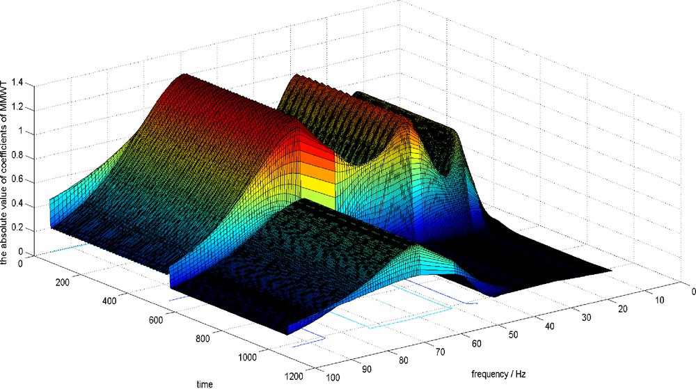
The absolute value of coefficients of MMWT of the data of Fig. 1.
Valeur absolue des coefficients de MMWT des données de la Fig. 1.

3.4 The wavelet transform coefficients of periodic function manifest periodic phenomenon w.r.t time variable for each scale

Let us suppose that the periodic signal is infinitely long. For the time series f_t : f_t = f_t+T(t ∈ Z), according to Eq. (11), we have

\begin{array}{l} {\bar{W}}_{f} (a, b) & = \frac{1}{a} \int_{- \infty}^{+ \infty} f (t) {\bar{ψ}}^{*} (\frac{t - b}{a}) d t \\ = \frac{1}{a} \int_{- \infty}^{+ \infty} f (t - T) {\bar{ψ}}^{*} (\frac{t - T - b}{a}) d t \\ = \frac{1}{a} \int_{- \infty}^{+ \infty} f (t) {\bar{ψ}}^{*} (\frac{t - T - b}{a}) d t \\ = {\bar{W}}_{f} (a, b + T) \end{array}

(34)

Thus we can say that the wavelet coefficients are also periodic w.r.t the time variable b (Yi and Fan, 2010).

From Eqs. (19) and (20), we can see the MWT and MMWT of the period function x₀(t) = cos(ω_ot), are periodic functions w.r.t time variable b with angular frequency ω₀, as long as we notice that ${\hat{ψ}}^{*} (a ω_{0})$ and ${\hat{\bar{ψ}}}^{*} (a ω_{0})$ are real.

The property is also valid for the signal with finite length, as long as the sampling frequency is high enough. Therefore, by analyzing the wavelet coefficients, we can obtain the periodicity of the signal.

3.5 The determination of the first and second periods by wavelet variance

The wavelet variance w.r.t MWT is defined (Yi and Fan, 2010) as

V (a) = \sum_{b} P_{W} f (a, b) = \sum_{b} | W_{f} (a, b) |^{2},

(35)

which measures the energy of f(t) at scale a because each P_Wf(a,b) measures the energy of f(t) in the Heisenberg box of each wavelet ψ_a,b centered at

(b, ξ = \frac{η}{a})

. In the same way, we can define the wavelet variance w.r.t MMWT as

\bar{V} (a) = \sum_{b} {\bar{P}}_{W} f (a, b) = \sum_{b} | {\bar{W}}_{f} (a, b) |^{2},

(36)

with which we will distinguish the first, second and other periodic components of the signal.

For a given signal, we have assumed the periodic items of the signal ${f (t_{i})}_{i = 1}^{T}$ with length T as

f (t) = c_{0} + \sum_{n = 1}^{N} c_{n} \cos (ω_{n} t) + d_{n} \sin (ω_{n} t)

(37)

where ω_n = n · 2π/T, n = 1, 2, …, N, and N is determined by the sampling period. We consider that the first period among all periodic components of the signal is the one with the most powerful energy that is determined by the oscillation amplitude and duration of the component. Now, we can distinguish the first, second periodic components of this signal with wavelet variance w.r.t MMPS (Yi and Fan, 2010). In fact, we have the following conclusion:

Theorem 3

For the periodic items(37)of a signal, let us denote the scale corresponding to the frequency ω_i, i = 1, 2, …, N by a_i, i = 1, 2, …, N, then the wavelet variance $\bar{V} (a_{i})$ w.r.t MMWT is proportional to the duration of the frequency ω_i, and is also proportional to the squared amplitude of the frequency component.

Proof Before calculating

\bar{V} (a_{i})

, we will make MMWT for g₁(t) = cos(ω_nt), and we can obtain

{\bar{W}}_{g_{1}} (a, b) = e^{i ω_{n} b} A

, where

A = e^{- \frac{σ^{2} {(a ω_{n} - η)}^{2}}{2}}

, according to (20). And we can also get

{\bar{W}}_{g_{2}} (a, b) = - i e^{i ω_{n} b} A

for g₂(t) = sin(ω_nt). From Eq. (36), we see the wavelet variance of f w.r.t MMWT is

\bar{V} (a) = \sum_{b} | {\bar{W}}_{f} (a, b) |^{2} = \sum_{b} | \sum_{n = 1}^{N} A e^{i ω_{n} b} (c_{n} - i d_{n}) |^{2}

(38)

where b = t₁, t₂, …, t_T. Because the scale corresponding to the frequency ω_i is a_i, we have

a_{i} = \frac{η}{ω_{i}}

according to Eq. (25). Now we will calculate V(a_i). When the index n of the summation is not equal to i, the value of

A = e^{- \frac{σ^{2} {(a_{i} ω_{n} - η)}^{2}}{2}}

is relatively small and can be temporarily neglected. When the index n of the summmation equals i, we have A = 1. So

\bar{V} (a_{i}) \approx T \cdot | c_{i} - i d_{i}) |^{2} = T \cdot (c_{i}^{2} + d_{i}^{2})

.

Therefore, the wavelet variance at scale a_i is proportional to the duration of the frequency component, and is also proportional to the squared amplitude of the frequency component, and as a result, we can estimate how much energy the signal with the frequency ω_i has by calculating $\bar{V} (a_{i})$ . In the following part of this paper, we will use wavelet variance w.r.t MMWT to distinguish the first and other periods of the time series while the wavelet variance w.r.t MWT can not achieve this goal.

In Fig. 3, the absolute value of coefficients of MMWT of a signal, physical activity is indicated at many scales, though the signal is locally monochromatic. For example, the Fig. 3, has nonzero values at many scales, but there are only three frequency components in the data. Although there is a “best” choice for the scale ${(a = a_{i})}_{i = 1,2,3}$ in the modulus, the nonzero correlations between the wavelets and data produce nonzero transform values at scales away from a_i. This can lead to confusion when trying to determine which period is present in the data; one method for dealing with this problem is that we can obtain all the periodic components of the time series by seeking for all the maximums of wavelet variance w.r.t MMWT instead of distinguishing the first and second periodic components strictly in accordance with the size of the wavelet variance (Yi and Fan, 2010).

We can obviously observe that the first period is the 60 Hz frequency component, whose amplitude is 1.2 in the first 512 samples and 0.6 in the latter 512 samples from the analytical expression of the original signal. And the second, third periods are the 30 Hz, 15 Hz components, whose amplitude is 1, 0.8 respectively, only appearing in the first 512 samples. However, the wavelet variance w.r.t MWT of 15 Hz, is larger than the wavelet variance of 30 Hz, according to the figure of wavelet variance w.r.t MWT in Fig. 4. At the same time, we can identify the size of the energy of each periodic component according to the figure of the wavelet variance w.r.t MMWT in Fig. 4. This is the third merit of MMWT compared with MWT.

Fig. 4
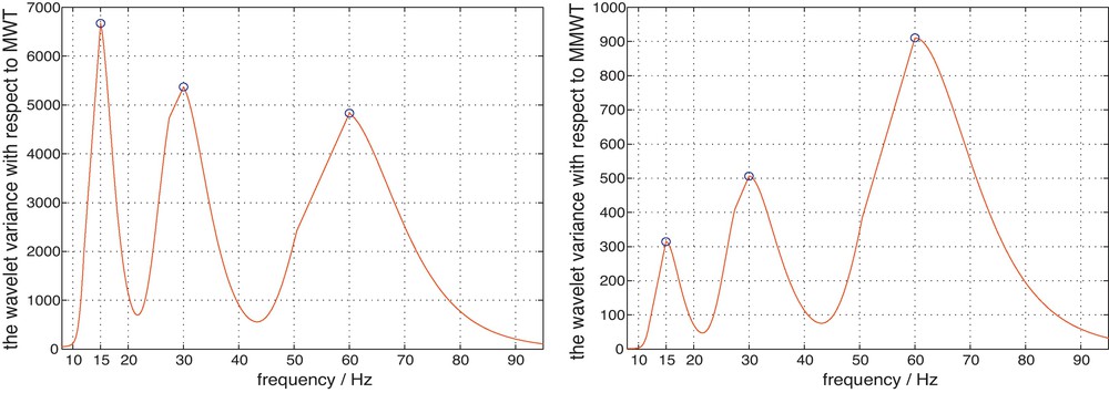
Wavelet variance w.r.t MWT and wavelet variance w.r.t MMWT for data of Fig. 1.
Variance d’ondelette w.r.t MWT et variance d’ondelette w.r.t MMWT pour les données de la Fig. 1.

So, in the following part of this article, we will only analyze the signal with MMWT.

4 Multi-period analysis of temperature data

Experiments have been made for daily average temperature measurements from January 1, 1951 to December 31, 2010, and the experimental site is No. 50978 weather station which is geographically set in Heilongjiang, in the Northeast of China. In geography, Heilongjiang is located in the East of continental Eurasia. In meteorology, Heilongjiang typically belongs to the warm climate zone with a continental monsoon climate, and is mainly distributed over the transition zone of east monsoon and arid inland. Economically, Northeast China is an important rice product base as well as a largest forest area in China. It is known that paddy rice and forest growth are heavily influenced by climate conditions. Obviously, the study of climate changes is valuable for agriculture and forest development in Northeast China. Furthermore, these local multiple periods can be used for creating multi-level spatiotemporal meteorological association rules in the system of spatiotemporal data mining Shu et al. (2009).

4.1 Global trend analysis

Generally, data preprocessing is necessary and important due to the nonlinear and nonstationary property of temperature time series. For example, as claimed by Capparelli et al. (2011), “long-term correlations can be masked by trends that can be generated by anthropic processes, e.g., the well-known urban warming, the increase of concentration of gases in the atmosphere, etc. For these effects, even uncorrelated data in the presence of long-term trends may appear correlated, and, on the other hand, long-term correlated data may look like uncorrelated data influenced by a trend.” So, detrended fluctuation analysis (DFA) was used to examine and compare the long-range correlations of fluctuations of total ozone and tropospheric brightness temperature and to determine if they exhibit persistent long-range correlations (Varotsos and Kirk-Davidoff, 2006). DFA was also applied on springtime daily column ozone (Varotsos, 2005). Furthermore, even if the DFA is used, the DFA result may be affected by the method of data preprocessing. For example, Capparelli et al. (2011) compared the DFA results for temperature anomalies defined in the classical way and through the empirical mode decomposition (EMD).

On the other hand, the advantage of the wavelet transform is that linear tendencies do not affect the transform. In fact, the wavelet transform is blind to lower-order polynomial behavior due to the vanishing moments of wavelets. As for the Morlet wavelet, the absolute value of MMWT of f(t) = 1 and f(t) = t, calculated according to (11), is so small compared with the computer round-off error that it is negligible as long as σ²η² ≫ 1. In spite of the theory analyzed above, linear trend is analyzed and removed before the identification of multi-scale time information of the data due to the fact that temperature data are generally a composite of a linear trend, periods, and a random signal.

From Fig. 5, we can calculate that the temperature was increasing over the last 60 years with an increasing rate of 0.00287°C/month. Unfortunately, the linear trend is not statistically significant, which may be caused by the 12 month period, the natural period, of the monthly temperature data.

Fig. 5
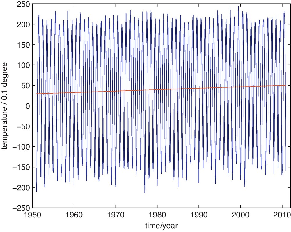
The monthly average temperature and the trend line of No. 50978 station (temperature on the vertical axis in Celsius degree of 0.1).
Température moyenne mensuelle et ligne de tendance pour la station 50978 (température en axe vertical en degré Celsius de 0,1).

From Fig. 6, we see that the temperature was increasing with an increasing rate of 0.3179 °C every ten years, which may be caused by intensive urban development in recent years. Moreover, the linear trend is statistically significant. In addition, Fig. 6 depicts the presence of the quasi-biennial oscillation (QBO) and the 11-year solar cycle in the time-series. In fact, local climate change must respond to the influence of global phenomena. The effect of solar cycle on climate has also been thoroughly discussed by Varotsos (1989) and Varotsos and Cracknell (2004).

Fig. 6
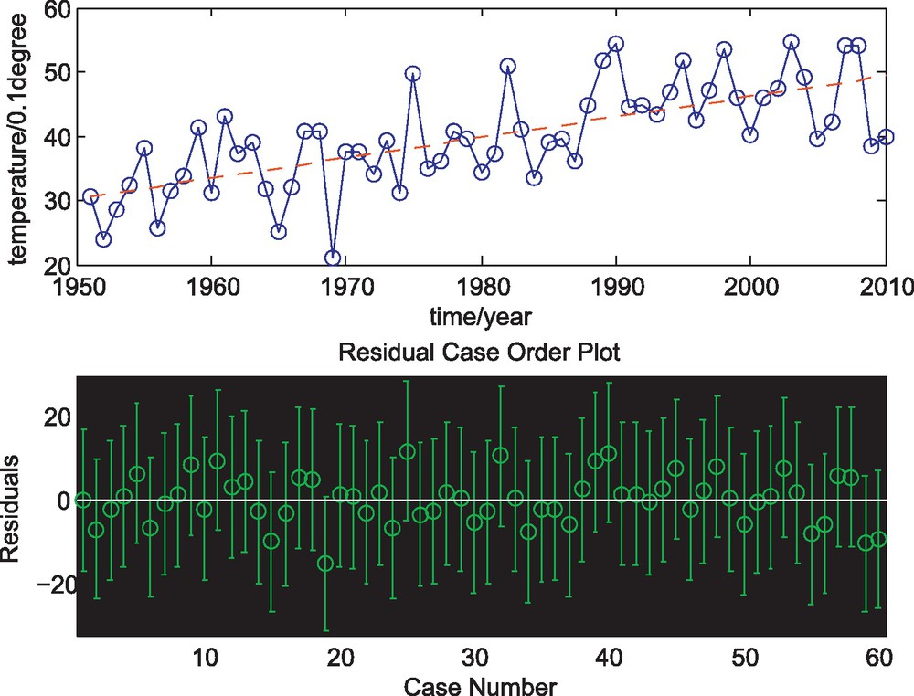
The first figure: the annual average temperature and the trend line for No. 50978 station. The second figure for the residual and confidence interval.
Première figure : température moyenne annuelle et ligne de tendance pour la station 50978. Seconde figure : intervalle résidual et de confiance.

4.2 The multi-period structure of the monthly average temperature data for No. 50978 station

The data analyzed in this section are the monthly average temperature data, and the length of data is 720 months, from January, 1951 to December, 2010 for No. 50978 station. After the removal of the linear trend, the MMWT of data is made. Fig. 7 is the contour of the real part of MMWT of temperature data. The rectangle in Fig. 7 highlights the negative and positive 12 month periodic oscillation, which is also illustrated in Fig. 8. The periodic oscillation of 12 months, which is the obvious periodic component in the data, is so strong that other periodic components cannot be detected with this method. Still, the ups and downs in the ridge of 12 month, shown in Fig. 8, indicate there exists other periodic components in the temperature data. Therefore, the annual average temperature data, which hides the 12 month periodic component, the natural period, will be analyzed in the following part.

Fig. 7
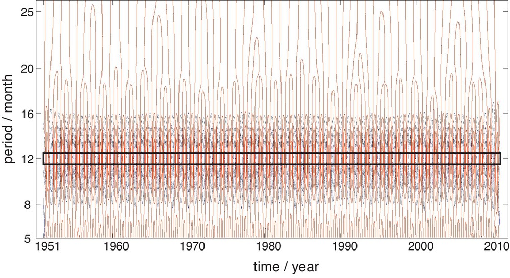
The contour of the real part of wavelet coefficients of the monthly average temperature of No. 50978 station. In this figure, the coefficients with negative values, which means the temperature is in cold stage, are plotted with dotted, blue line. While the coefficients with positive values, which means the temperature is in warm stage, are plotted with dashed, red line. And so it is easily seen that the 12 month period lasts 60 cycles as long as we notice that an interchange between warm stage and cold stage means a cycle.
Contour de la part réelle des coefficients d’ondelette de la température moyenne mensuelle de la station 50978. Dans cette figure, les coefficients qui ont des valeurs négatives – ce qui signifie que les températures corréspondent à une phase froide – sont représentés par une ligne bleue pointillée, tandis que les coefficients à valeur positive – ce qui signifié que les températures correspondent à une phase chaude – sont représentés par une ligne rouge tiretée. Ainsi, il est facile de constater qu’une période de 12 mois dure 60 cycles, si l’on considère que le changement entre phase chaude et phase froide constitue un cycle.

Fig. 8
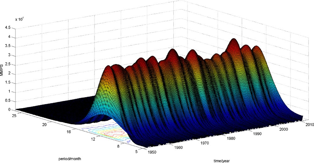
The MMPS of the monthly average temperature.
MMPS de la température moyenne mensuelle.

4.3 The multi-period structure of the annual average temperature data for No. 50978 station

The data analyzed in this section are the annual average temperature data, and the length of data is 60 years, from 1951 to 2010 for No. 50978 station. The data and the trend line are shown in Fig. 6. Still, the linear trend is removed before MMWT of the data is done. Then the possible periods range from 2 year to 60 year by Nyquist sampling theorem since the sampling period is 1 year and the length of data is 60 years (Yi and Fan, 2010). Instead of the method proposed by Yi and Fan (2010), the scales adopted in this experiment are determined by periods of 2^1+0/96, 2^1+1/96, 2^1+2/96, …, 2^1+471/96 years according to scale-to-frequency formula (25), which means that there are 96 intermediate scales in each octave [2^j,2^j+1] (Mallat, 2009). Then the wavelet variance w.r.t MMWT of the data is shown in Fig. 9 and the periodic components embedded in the data are obtained by seeking for all the maximums of wavelet variance. Instead of the integer periodic components obtained in Yi and Fan (2010), the 4.0290, 6,5357, 14.9933, 32.2319 year periods are obtained and the first, second, …, fourth approximate integer periods are 4, 7, 15, 32 year according to the size of their wavelet variance. The rectangles in Fig. 10, the contour of the real part of MMWT of the data, highlight the four dominant periodic oscillations. In fact, in Fig. 10, the coefficients with negative values are plotted with dotted, blue line, which means that the temperature is in cold stage. And the coefficients with positive values are plotted with dashed, red line, which means that the temperature is in warm stage. And so the negative and positive oscillation of local time structures of the annual average temperature, the different dominant time scales in different time intervals, are visualized clearly, and can be analyzed through four aspects.

Fig. 9
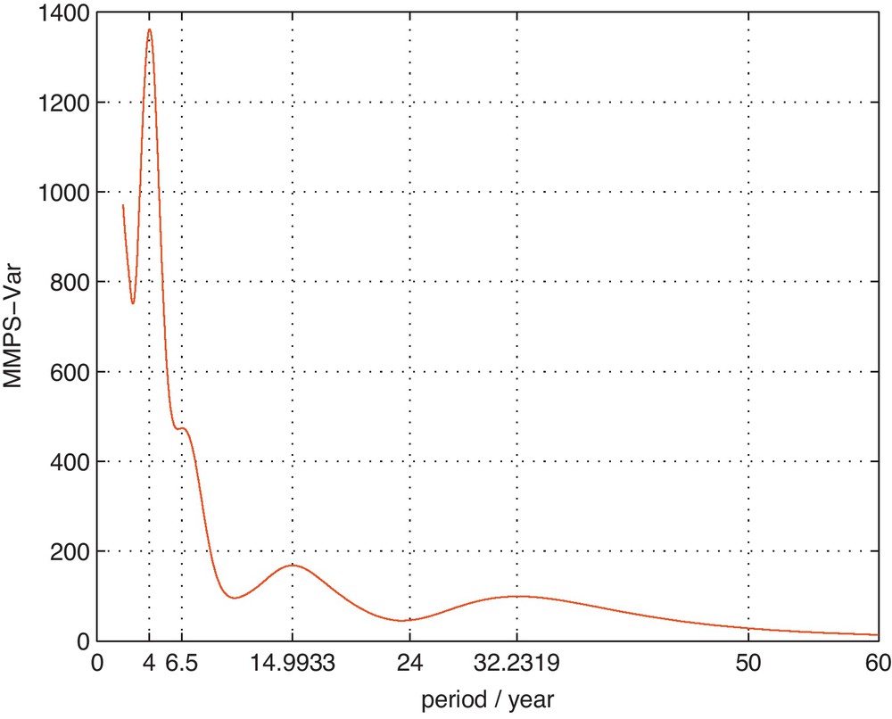
The wavelet variance w.r.t MMWT of the annual temperature data for No. 50978 station.
Variance d’ondelette w.r.t MMWT des données de température annuelle pour la station 50978.

Fig. 10
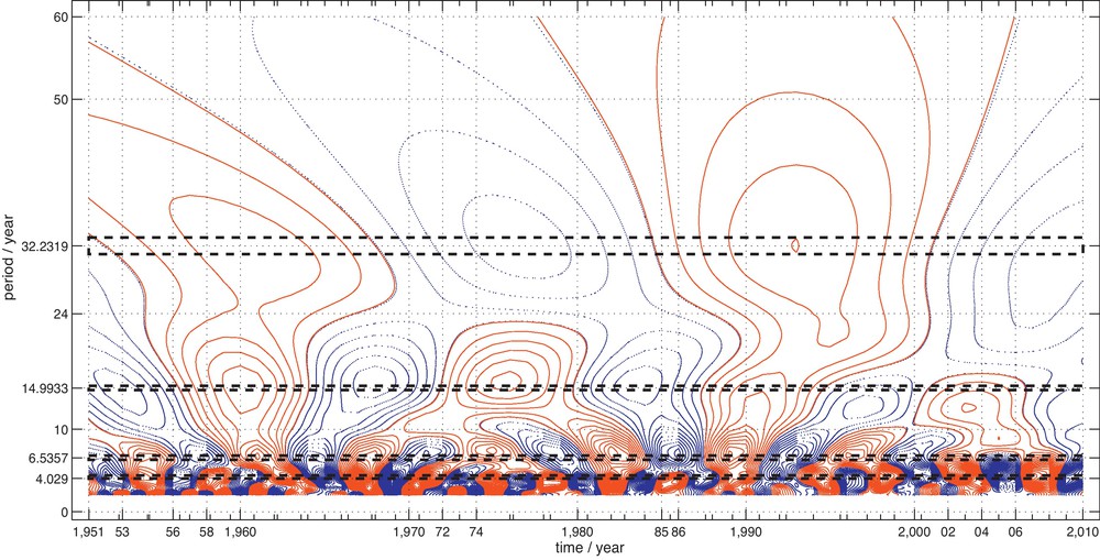
The contour of the real part of coefficients of MMWT of the annual average temperature for No. 50978 station. In this Figure, the coefficients with negative values are plotted with dotted, blue line, while the coefficients with positive values are plotted with dashed, red line.
Contour de la part réelle des coefficients de MMWT de la température moyenne annuelle pour la station 50978. Les coefficients à valeur négative sont représentés par une ligne bleue pointillée et les coefficients à valeur positive par une ligne rouge tiretée.

First of all, it is seen from Fig. 10 that besides the four dominant periods, the other periods are transitional periodic components, and almost all periods are globally apparent and undergo cold and warm interchanging time intervals. In particular, the isolines of the negative coefficients for almost all periods in recent years are not closed, and this indicates that the temperature in the cold stage may be predicted in the upcoming years for all time scales.

Secondly, for some time intervals, it may manifest a warm stage for a certain scale, and may manifest a cold stage for another scale. The result is listed in Table 2.

Period (year)	4–7	15	32–54	Period (year)	4	7	11–48
1953–1955	Warm	Cold	Warm	1958–1959	Warm	Cold	Warm
Period (year)	4	6–24	28–60	Period (year)	11–15	17–32
1985–1986	Warm	Cold	Warm	2002–2006	Warm	Cold
Period (year)	11–23	24–52
1973–1980	Warm	Cold

Thirdly, we give a detailed analysis for the four dominant periods. The first map of Fig. 11, a local part of Fig. 10, focus on the regularly 4 year periodic oscillations, and the second map of Fig. 11, the real part of the wavelet coefficients of 4.0290 year periodic component, vividly mimic the 4 year temperature fluctuation and last about 15 cycles. The minimum negative coefficient is −6.5778 (unit: 0.1°C) occurring in 1969, the maximum positive coefficient 6.8375 (unit: 0.1 °C) occurring in 1967⁴. The comparisons between the maximum and minimum wavelet coefficients of the four dominant periods are listed in Table 3.

Number of years	Minimum coefficient	Time	Maximum coefficients	Time
4	−6.5778	1969	6.8375	1967
7	−4.2296	1969	4.0977	1989
15	−2.1422	1968	2.1341	1960
32	−1.3380	1977	1.4984	1993

From the first map of Fig. 12, a local part of Fig. 10, focusing on the 6.5357 year periodic oscillations, it can be concluded that this period component lasts about nine cycles as long as we notice that an interchange between cold and warm takes place in a cycle in the contour map. The second map of Fig. 12 gives us an image of periodic fluctuation.

Fig. 12
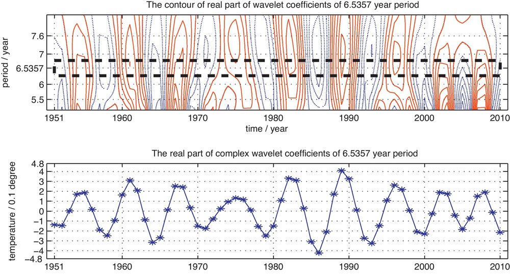
The wavelet coefficients of 6.5357 year period.
Coefficients d’ondelette de période de 6,5357 ans.

The third period, the 14.9933 year periodic oscillations, is depicted in Fig. 13. The very regular cycle oscillation is apparent.

Fig. 13
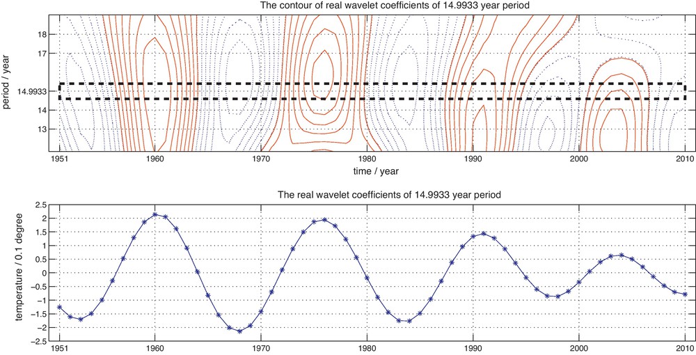
The wavelet coefficients of 15.1020 year periodic components.
Coefficients d’ondelette des composants à période de 15,1020 ans.

The fourth period, the 32.2319 year periodic oscillations, is depicted in Fig. 14. The cycle oscillations last very regularly about 2 cycles, and the warm, cold and warm, cold interchanges are apparent in this figure.

Fig. 14
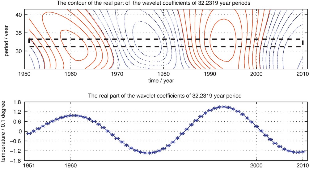
The wavelet coefficients of 32.2319 year periodic components.
Coefficients d’ondelette des composants à période de 32,2319 ans.

Unlike the Fourier periodic components such as sinusoidal signals, which have constant amplitudes through all the time, the amplitudes of the four dominant periods fluctuate in a small range from time to time. We can distinguish the most striking time intervals of periodic oscillations by resorting to Fig. 15, the contour of MMPS of the annual average temperature for No. 50978 station, and the result is listed in Table 4.

Fig. 15
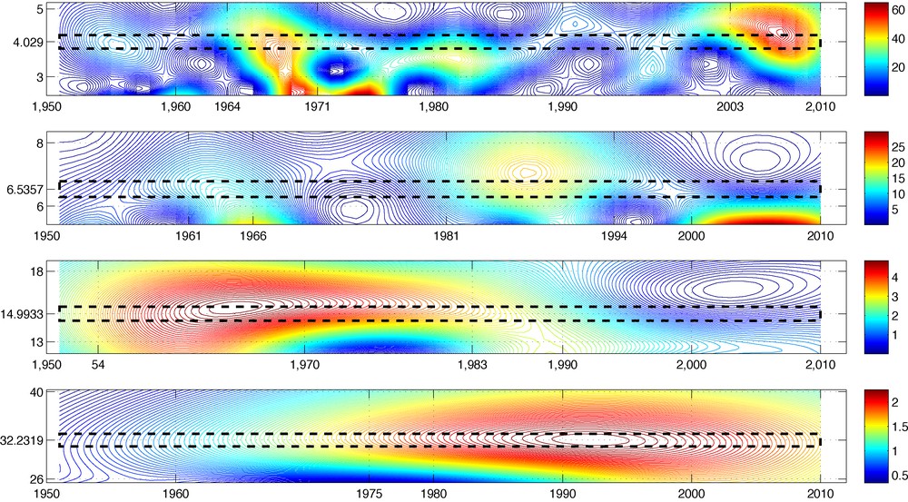
The contour of MMPS of the annual average temperature for No. 50978 station.
Contour de MMPS de la température moyenne annuelle pour la station 50978.

Period (year)	4.0290	14.9933
Time intervals	1964–1971 and 2003–2010	1954–1983
Period (year)	6.5357	32.2319
Time intervals	1961–1966 and 1981–1994	1975–2010

4.4 The relationship between wavelet coefficients of the annual average temperature and the monthly average temperature for No. 50978 station

A comparison between the real part of wavelet coefficients of 48.3480 month (4.0290 year) period, obtained from the monthly average temperature, and of 4.0290 year period, obtained from the annual average temperature, is given in Fig. 16, because of the fact that the periodic oscillation of 12 month, analyzed in Section 4.2, is the only one periodic component in the monthly average temperature, and in Section 4.3, the first period of the annual average temperature is 4.0290 year. It is seen that the amplitudes and oscillation trends of two maps in Fig. 16, are similar except that the first map is composed of 720 points (month) and the second 60 points (year). So it is necessary that MMWT should be tested by removing the 12 month period and analyzing the residuals.

Fig. 16
The relationship between the real wavelet coefficients of the monthly average temperature and the annual average temperature for No. 50978 station.
Relation entre coefficients d’ondelette réels de la température moyenne mensuelle et de la température moyenne annuelle pour la station 50978.

5 Conclusion

The multi-period analysis is important for the study of climate change. Up until now, the efficient methods are lacking for this work. In this regard, We make some explorations and obtain some new findings.

Firstly, by introducing Morlet wavelets with shape parameter, the following results are given:

• there is a unique and unambiguous interpretation of scale as frequency for the MMWT, while difference exists for the MWT;
• MMWT maintains the same amplitude between the original frequency component and the wavelet coefficients;
• the wavelet transform coefficients of periodic function manifest periodic phenomenon w.r.t time variable for each scale;
• the wavelet variance w.r.t MMWT is proportional to the duration of the frequency component and is also proportional to the amplitude squared of the frequency component. The four results are useful in multi-period analysis of time series.

Secondly, the multi-period structure of temperature data for No. 50978 station are analyzed. For the monthly average temperature data, the 12 month period is so strong that other periodic components can not be detected. For the annual average temperature data, the 4, 7, 15, 32 year periods are the four dominant periods and the amplitudes of these periods are quantitatively given by wavelet coefficients by taking advantage of MMWT. The interchanges between the cold and warm oscillation of temperature are apparent in the real part of MMWT. The temperature in the cold stage may be predicted in the upcoming years for all time scales. In our system of spatiotemporal data mining, these local multiple periods can be used for creating multi-level spatiotemporal meteorological association rules.

Acknowledgment

We sincerely thank the anonymous reviewers for their constructive comments to enhance the quality of the manuscript.

¹ So this wavelet is admissible by calculation that $\hat{ψ} (0) = 0$ . Furthermore, the theoretical analyses in the following part of this article for two definitions of mother wavelet are almost the same.

² The introduction of the sampling frequency is necessary when we analyze the discrete signal. In fact, if we neglect the sampling frequency dt in Theorem 1 or in the equation (27), some errors may be produced. For example, in Table 1, the quantitative values of the row “the amplitude w.r.t MWT” is calculated from Eq. (27), and in this calculation, dt, the sampling time of the signal in Fig. 1 of this paper, is $\frac{1}{400}$ . It is obvious that if the sampling time in Eq. (27) is not introduced, the corresponding values in Table 1 will be wrong, and will contradict with Fig. 2.

Fig. 1
A synthetic signal with length 1024. The first half contains sinusoidal signal superimposition with three different frequencies, namely 0.8 sin (30πt) + sin (60πt) + 1.2 sin (120πt). The latter half contains the 60 Hz sinusoidal signal with amplitude 0.6, namely 0.6 sin (120πt). Here the sampling frequency is 400 Hz.
Signal synthétique de longueur 1024. La première moitié comporte la superposition du signal sinusoïdal avec trois fréquences différentes. L’autre moitié comporte le signal sinusoïdalde 60 Hz avec une amplitude de 0,6. La fréquence est ici de 400 Hz.

Fig. 2
The absolute value of coefficients of MWT of the data of Fig. 1.
Valeur absolue des coefficients de MWT des données de la Fig. 1.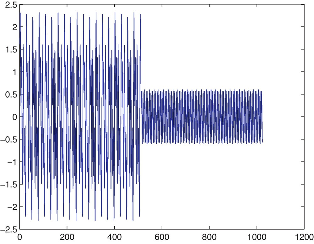

	15 Hz	30 Hz	60 Hz	60 Hz
The original amplitude	0.8	1	1.2	0.6
The amplitude w.r.t MWT	3.4864	3.0815	2.6148	1.8489
The amplitude w.r.t MMWT	0.8	1	1.2	0.6

³ It is not necessary to introduce the sampling time dt in Theorem 2 while it is necessary in Theorem 1, which may be another merit of MMWT compared with MWT.

⁴ Wavelet coefficients are endowed with the unit of temperature due to the fact that the quantitative depict of each period of data is given by taking advantage of MMWT.

Fig. 11
The real part of wavelet coefficients of 4.0290 year period.
Part réelle des coefficients d’ondelette de période de 4,0290 ans.

Bibliographie

[Capparelli et al., 2011] V. Capparelli; A. Vecchio; V. Carbone Long-range persistence of temperature records induced by long-term climatic phenomena, Phys. Rev. E, Volume 84 (2011), p. 046103

[Carmona et al., 1998] R. Carmona; W. Hwang; B. Torrésani Practical time-frequency analysis: Gabor and wavelet transforms with an implementation in S, Acad. Press, Volume 9 (1998)

[Chattopadhyay and Chattopadhyay, 2012] G. Chattopadhyay; S. Chattopadhyay Monthly sunspot number time series analysis and its modeling through autoregressive artificial neural network, Eur. Phys. J. Plus, Volume 127 (2012), pp. 1-8

[Chattopadhyay et al., 2011] G. Chattopadhyay; S. Chattopadhyay; P. Chakraborthy Principal component analysis and neurocomputing-based models for total ozone concentration over different urban regions of India, Theory Appl. Climatol. (2011), pp. 1-11

[Delprat et al., 1992] N. Delprat; B. Escudie; P. Guillemain; R. Kronland-Martinet; P. Tchamitchian; B. Torresani Asymptotic wavelet and Gabor analysis: Extraction of instantaneous frequencies, IEEE Trans. Inform. Theory, Volume 38 (1992), pp. 644-664

[Grossmann and Morlet, 1984] A. Grossmann; J. Morlet Decomposition of hardy functions into square integrable wavelets of constant shape, Soc. Indust. Appl. Math., Volume 15 (1984), pp. 4093-4100

[Guillemain et al., 1991] P. Guillemain; R. Kronland-Martinet; B. Martens Estimation of spectral lines with the help of the wavelet transform: application in the NMR spectroscopy (Y. Meyer, ed.), Research Notes in Applied Mathematics: Wavelet and Applications, Masson-Springer-Verlag, Paris, 1991, pp. 48-60

[Huang, 2004] M. Huang Wave parameters and functions in wavelet analysis, Ocean Engin., Volume 31 (2004), pp. 111-125

[Issac et al., 2004] M. Issac; G. Renuka; C. Venugopal Wavelet analysis of long period oscillations in geomagnetic field over the magnetic equator, J. Atmos. Solar Terrest. Phys., Volume 66 (2004), pp. 919-925

[Labat, 2005] D. Labat Recent advances in wavelet analyses: Part 1 – a review of concepts, J. Hydrol., Volume 314 (2005), pp. 275-288

[Labat et al., 2005] D. Labat; J. Ronchail; J. Guyot Recent advances in wavelet analyses: Part 2 – Amazon, Parana, Orinoco and Congo discharges time scale variability, J. Hydrol., Volume 314 (2005), pp. 289-311

[Lilly and Olhede, 2009] J. Lilly; S. Olhede Higher-order properties of analytic wavelets, IEEE Trans. Signal Process, Volume 57 (2009), pp. 146-160

[Lin and Qu, 2000] J. Lin; L. Qu Feature extraction based on Morlet wavelet and its application for mechanical fault diagnosis, J. Sound Vib., Volume 234 (2000), pp. 135-148

[Mallat, 2009] S. Mallat A wavelet tour of signal processing, Academic Press, 2009

[Meyers et al., 1993] S. Meyers; B. Kelly; J. O’Brien An introduction to wavelet analysis in oceanography and meteorology: With application to the dispersion of Yanai waves, Month. Weather Rev., Volume 121 (1993), pp. 2858-2866

[Saracco et al., 1991] G. Saracco; J. Sessarego; J. Sageloli; P. Guillemain; R. Kronland-Martinet et al. Extraction of modulation laws of elastic shells by the use of the wavelet transform (Y. Meyer, ed.), Wavelets Appl., Masson-Springer, 1991, pp. 61-68

[Saracco et al., 2009] G. Saracco; N. Thouveny; D. Bourlès; J. Carcaillet Extraction of non-continuous orbital frequencies from noisy insolation data and from palaeoproxy records of geomagnetic intensity using the phase of continuous wavelet transforms, Geophys. J. Int., Volume 176 (2009), pp. 767-781

[Shu et al., 2009] Shu, H., Guo, K., Zhang, H., 2009. Multiscale analysis of climate data in ChangChun, Proceedings of SPIE. Int. Soc. Opt. Eng. 7498.

[Shyu and Sun, 2002] H. Shyu; Y. Sun Construction of a Morlet wavelet power spectrum, Multidimensional Syst. Signal Process., Volume 13 (2002), pp. 101-111

[Torrence and Compo, 1998] C. Torrence; G. Compo A practical guide to wavelet analysis, Bull. Am. Meteorol. Soc., Volume 79 (1998), pp. 61-78

[Varotsos, 1989] C. Varotsos Comment on connections between the 11-year solar cycle, the qbo and total ozone, J. Atmos. Terrest. Phys., Volume 51 (1989), pp. 367-370

[Varotsos, 2005] C. Varotsos Power-law correlations in column ozone over Antarctica, Int. J. Remote Sensing, Volume 26 (2005), pp. 3333-3342

[Varotsos and Kirk-Davidoff, 2006] C. Varotsos; D. Kirk-Davidoff Long-memory processes in ozone and temperature variations at the region 60̊S-60̊N, Atmos. Chem. Phys., Volume 6 (2006), pp. 4093-4100

[Varotsos and Cracknell, 2004] C.A. Varotsos; A.P. Cracknell New features observed in the 11-year solar cycle, Int. J. Remote Sensing, Volume 25 (2004), pp. 2141-2157

[Werner, 2008] R. Werner The latitudinal ozone variability study using wavelet analysis, J. Atmos. Solar Terrest. Phys., Volume 70 (2008), pp. 261-267

[Yi and Fan, 2010] Yi, H., Fan, Q., 2010. An algorithm for the determination of multi-period structure of time series, IEEE International Conference on Information and Automation (ICIA) 1684–1689.

[Yi et al., 2010] H. Yi; H. Shu; T. Zhang; Q. Fan Applications of Morlet wavelets in time-frequency localization of signals, Math. Appl., Volume 23 (2010), pp. 395-400

^☆ This work is jointly supported by the National Natural Science Foundation of China (No. 41171313) and the National Basic Research Program of China (973 Program) (No. 2011CB707103).

Commentaires - Politique