


 CC-BY 4.0
1. Introduction
The Earth’s Critical Zone (CZ) is the near-surface layer where water, soil, air, and living organisms interact to support terrestrial ecosystems and human society. Among its components, groundwater (GW) represents the largest reservoir of freshwater (Singha and NavarreSitchler, 2022; R. M. Lee et al., 2023). It plays a fundamental role in Earth’s hydrogeochemical cycles by redistributing water, energy, solutes, and contaminants throughout the subsurface (Brunke and Gonser, 1997; Stegen et al., 2018; Gomez-Gener et al., 2021). In addition to sustaining ecosystems and surface water (SW) bodies critical to biodiversity, GW is a vital resource for global water, energy, and food security (De Amorim et al., 2018; Castilla-Rho et al., 2017; Saccò et al., 2024).
Despite its significance within the Critical Zone (CZ), GW is frequently overlooked due to the difficulty and high cost of subsurface access, and its characteristically slow, diffuse dynamics (Chavez Garca Silva et al., 2024). Hydrogeophysical methods provide efficient, non-intrusive tools to estimate GW physical properties in time and space. However, key challenges in CZ hydrogeophysics include: (i) characterizing the structure and behavior of GW systems and their interactions with other CZ compartments, (ii) quantifying the temporal and spatial distribution of water, energy, and nutrients or contaminants, and (iii) predicting GW responses to climatic variability and anthropogenic influences.
Shallow GW systems are influenced by both climatic factors (Cuthbert et al., 2019; Fan et al., 2013; Condon, Atchley, et al., 2020) and anthropogenic pressures such as water abstraction (Dixon et al., 2006; Rahardjo et al., 2010; Waltham et al., 2004), geothermal exploitation (Bidarmaghz et al., 2021; Menberg et al., 2025; Bayer, Attard, et al., 2019), and contaminant discharge (Stigter et al., 2023). In this context, understanding long-term trends and the spatial dynamics of GW recharge, SW–GW exchanges, flow paths, residence times, and associated thermal regimes is essential for anticipating future conditions and managing current impacts (Maxwell and S. J. Kollet, 2008; De Marsily, 1986; Enemark, Peeters, et al., 2019; Boulton and Hancock, 2006; Singha and NavarreSitchler, 2022; Gleeson et al., 2020; Fan et al., 2013). Temperature is increasingly recognized as a key tracer in shallow GW systems, providing critical insights into water quality, recharge dynamics, and geothermal potential (Neidhardt and Shao, 2023; Xu et al., 2021; Benz et al., 2024). Although only a limited number of studies have focused on temperature evolution within GW, recent investigations underscore its sensitivity to climatic variability and anthropogenic pressures (Benz et al., 2024). Water and temperature are fundamental vectors of transport and transformation within the CZ, shaping biogeochemical processes that influence CZ functioning (Safieddine et al., 2025), altering water quality through complex biogeochemical feedbacks (Neidhardt and Shao, 2023), and affecting stream and GW biodiversity (Land and Peters, 2023).
Unraveling the four-dimensional (4D) distribution of water and heat fluxes at the GW boundaries (i.e. 3D spatial + temporal), particularly at the Vadose Zone (VZ) and SW–GW interfaces (Hermans, Goderniaux, et al., 2023) remains a major challenge for accurately assessing the components of the water and energy balances and achieving water budget closure, particularly concerning climate changes and land use (Blöschl et al., 2019; Condon, S. Kollet, et al., 2021; Xie, Cook, et al., 2018; Xie, Crosbie, et al., 2019; Levin et al., 2023). VZ regulates recharge, vertical water movement, and the exchange of energy and solutes, while SW–GW interactions control hydrological connectivity as well as the magnitude and directionality of both water and thermal exchanges. These efforts are further complicated by the non-linear, transient nature of GW recharge processes, including capillary rise across the water table (Vereecken, Huisman, et al., 2008), shifting GW divides that can induce lateral flows between riverbanks (Texier et al., 2022), and temporally variable SW–GW connectivity. SW–GW can fluctuate between gaining, losing, transitional, and disconnected states, introducing uncertainty into water and energy budget estimation (Brunner, Therrien, et al., 2017; Brunner, Cook, et al., 2011; Rivière, Gonçalvès, Jost and Font, 2014) (Figure 1).
(a) Watershed-scale view illustrating GW flow paths, geological structure, SW–GW interactions, and human influences, with idealized GW divides and flowpaths (after Tóth, 1963). (b) Hillslope-scale 3D view with subsurface hydrofacies heterogeneity meshes, model parameters (intrinsic permeability k, porosity n, specific yield Sy, water retention curve WRC (Van Genuchten, 1980; Mualem, 1976; Brooks and Corey, 1966; Fredlund, 2006), thermal conductivity 𝜆, the density of the porous media 𝜌 and heat capacity C). Parameters may vary continuously or discretely across the domain, reflecting natural heterogeneity and modeling assumptions. (c) Output of advanced GW simulation following data integration and inversion (Inv), revealing realistic SW–GW flow paths, residence time distribution, and estimates of water and heat budgets. After inversion, spatial uncertainty in model parameters and flow directions can be quantitatively assessed, reflecting the limitations imposed by sparse or uneven field data. FWD: forward models; Inv: inversion approaches.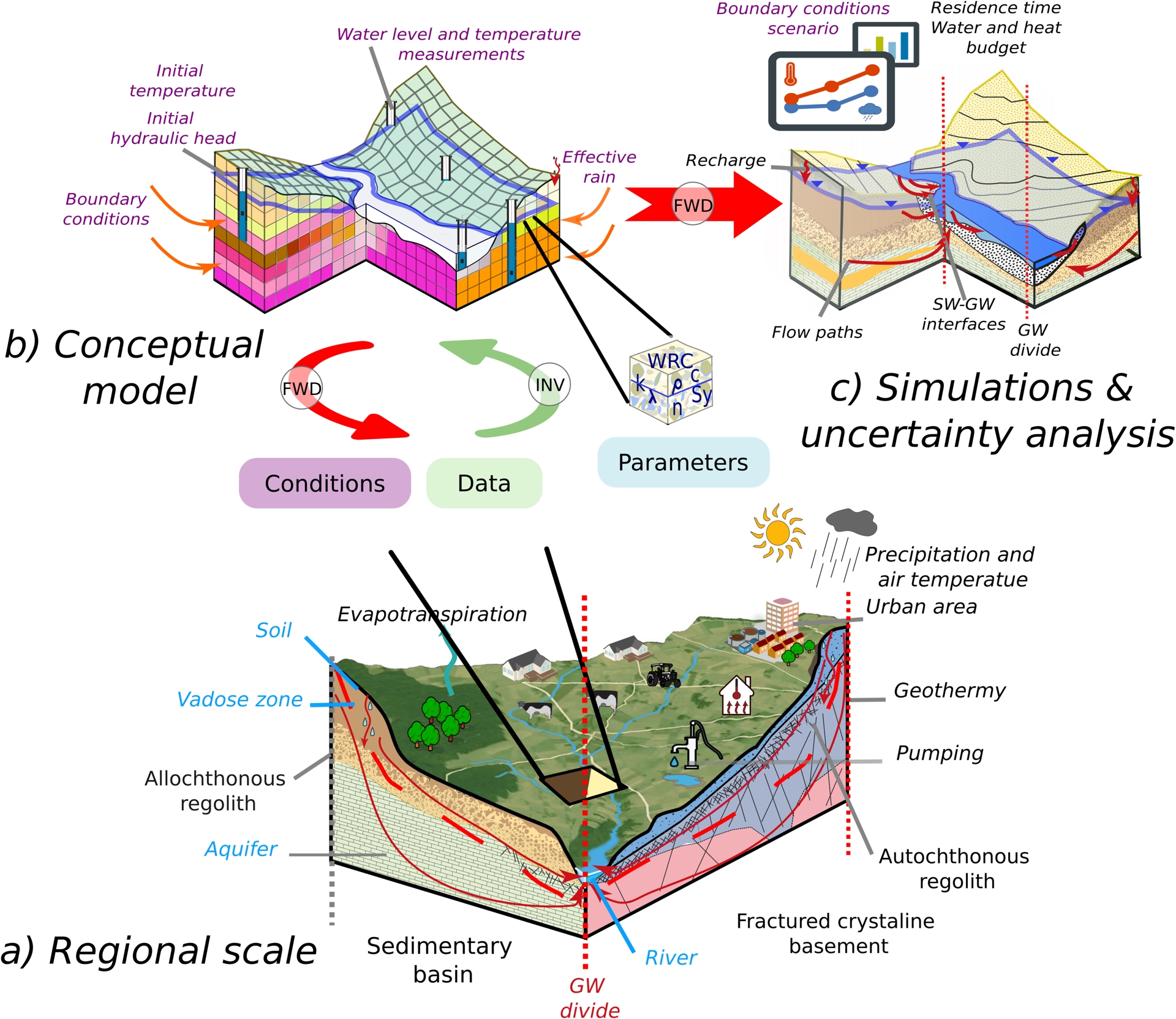
GW flow systems remain poorly understood due to their hidden subsurface nature, often described as a terra incognita (Kleinhans et al., 2005; McDonnell, 2017; Grant and Dietrich, 2017) (Figure 1). Shallow GW systems exhibit a rich diversity in the composition and topology of internal structures, shaped by interactions among geological, hydrological, and climatic processes (see Appendix A). These systems are underlain by regolith, which can be categorized into two types: allochthonous regolith, composed of unconsolidated sediments transported through geomorphological mechanisms, and autochthonous regolith, formed through in-situ weathering and transformation of the underlying bedrock. The evolution of regolith and bedrock varies significantly across spatial and temporal scales, complicating the accurate representation of flow and transport dynamics (further detailed in Appendix A). Despite the advancement of hydrogeological modeling, GW management, including well regulation, streamflow depletion, recharge enhancement, and development of geothermal resources, often operates under significant data constraints. These limitations require simplifying assumptions that can obscure spatial heterogeneity, misrepresent boundary conditions, and ultimately lead to non-unique or unreliable model interpretations (Casillas-Trasvina et al., 2024). However, the hydrological sciences have historically prioritized hydraulics and mathematical modeling over geological realism, frequently yielding precise solutions to ill-posed problems. Inadequate conceptual geological models and poor estimations of aquifer parameters still contribute to major sources of uncertainty in flow modeling (Rojas et al., 2010; Refsgaard et al., 2012; Enemark, Peeters, et al., 2019; Yin et al., 2021; D.-H. Tran et al., 2025).
While many components of the hydrological cycle, such as river discharge, precipitation, piezometric levels, and even GW pumping (though often not routinely monitored), can be measured with reasonable accuracy, fluxes at GW boundaries, including recharge (Rawls et al., 1993; Halloran et al., 2016; W. Zheng et al., 2019; Vereecken, Amelung, et al., 2022) and SW–GW exchanges (Fleckenstein, Krause, et al., 2010; Krause et al., 2011; Flipo et al., 2014; Barthel, 2014; Boano, J. W. Harvey, et al., 2014; Irvine et al., 2024), cannot be directly observed at the hillslope scale. Although methods such as seepage meters (Rosenberry, Duque, et al., 2020), lysimeters (Saaltink et al., 2020; Balugani et al., 2023; Saaltink et al., 2020), single-well tracer tests (Paradis et al., 2022), and active Distributed Temperature Sensing (DTS) experiments (Chang et al., 2024; Briggs, Lautz, et al., 2012) are often described as “direct measurements” of these fluxes (Rosenberry and LaBaugh, 2008), they actually infer exchange rates by inverting data. Each inversion requires modeling assumptions and is sensitive to site-specific conditions. While informative at the local scale, such measurements are rarely representative of larger domains.
At the hillslope or watershed scale, SW–GW exchanges are often depicted using a one-dimensional conductance term in watershed models. This representation neglects heterogeneity and assumes steady-state conditions and places the GW divide at the midpoint of the river (Gianni et al., 2016). This conceptual limitation is illustrated in Figure 1a, which shows how GW flow paths and divides are idealized without accounting for hydrofacies variability. Notably, if the transient state is not taken into account, predictions of exchange fluxes will be unreliable, especially during extreme events (Tripathi et al., 2021). This limitation impacts water fluxes as well as heat and solute transport processes (Lemoubou et al., 2023). In reality, GW head distributions follow physical laws that yield complex spatial patterns, which are not easily reproduced with analytical solutions or simplified geometries. Consequently, assigning boundary conditions based on topography or interpolation of piezometric level carries a significant risk of physical inconsistency (De Marsily, Delay, Gonçalvès, et al., 2005). A major unresolved issue remains the inherent incompleteness of the data required to constrain these models accurately.
Figure 1 provides a conceptual overview of GW systems at multiple scales, illustrating (a) watershed-scale flow paths and human influences, (b) hillslope-scale subsurface heterogeneity and hydrogeological parameters, and (c) the output of advanced GW simulations and inversion approaches, which estimate GW flow paths, residence times, SW–GW exchanges, and recharge across the domain. The fundamental challenge lies in solving flow and transport equations within a complex geological system that remains only partially characterized (Anderson, Woessner, et al., 2015). Parameters may vary continuously or discretely across the domain. In both cases, the subsurface domain is discretized into a mesh of cells in the model. Each mesh assigned a set of parameters that defines the hydraulic and thermal behavior of the medium (Figure 1b). These parameters such as the saturated hydraulic conductivity (or permeability), porosity, the relative permeability function, water retention curve, unsaturated permeability function, specific heat (heat capacity/density), thermal conductivity, and density of every phase (i.e., solid particles, water, and air) are typically linked to a specific hydrofacies, which represent geologically coherent units with distinct properties. While this framework enables spatial variability in model inputs, it also depends heavily on how well the hydrofacies are conceptualized, parameterized, and distributed (Zinn and C. F. Harvey, 2003; Zhan et al., 2023), underscoring the importance of robust geological characterization. Although heterogeneity is incorporated into models at a certain scale, it is not directly observed or mapped in detail at the scale of the cell of the model (Figure 1b). Instead, its spatial distribution is typically inferred from sparse measurements through inverse modeling or interpolated through a geostatistical framework, introducing further uncertainty into the representation of subsurface complexity (Condon, S. Kollet, et al., 2021; H. Zhou et al., 2014).
As a result, GW simulations often reflect a compromise between (Gupta et al., 2012): (i) available data and its spatiotemporal resolution (Irvine et al., 2024; Condon, S. Kollet, et al., 2021; De Marsily, Combes, et al., 1992; Konikow and Bredehoeft, 1992; Andréassian et al., 2023; Carrera et al., 1993); (ii) the complexity of physical processes; (iii) model capacity to represent heterogeneity and boundary conditions; and (iv) the inclusion of uncertainties in model inputs, structure, parameters, and observations used to constrain model parameter sets (Condon, S. Kollet, et al., 2021; H. Zhou et al., 2014; Sagar et al., 1975; Tarantola, 2006) (Figure 1c).
Most hydrological models are calibrated using two conventional observation types: hydraulic heads and river discharge. However, it is established that these conventional observations alone are insufficient to accurately parameterize subsurface heterogeneity and predict flow paths and transport dynamics, especially in geologically complex settings and near the SW (De Marsily, Delay, Gonçalvès, et al., 2005). Calibration from hydraulic heads alone often leads to non-unique solutions (Beven, 2006; Doherty, 2011). This issue arises because distinct hydrofacies can produce similar hydraulic responses but different flow paths.
To illustrate the hydrogeological consequences of sedimentary heterogeneity, Figure 2 presents a hydrogeological simulation of GW flow paths and hydraulic gradients within a synthetic geological model of a meandering fluvial system. The geological model, developed using the Flumy process-based sedimentary simulator, mimics the deposits in a simplified alluvial plain (Weill et al., 2013; Bhavsar et al., 2024). The facies simulated by Flumy were implemented in a GW flow model to assess the impact of mud plugs, which are low-permeability deposits formed in abandoned meanders, on subsurface flow dynamics. Modeling details are provided in Appendix A. The results show that while the overall hydraulic head distributions in the homogeneous and heterogeneous models appear nearly identical, the presence of mud plugs significantly alters GW flow directions and locally doubles the velocity beneath these features. These insights underscore the limitations of relying solely on hydraulic head data for model calibration.
Sedimentary and hydrogeological setup (facies and hydrological boundary conditions): (a) homogeneous sedimentary model, (b) heterogeneous sedimentary model, (c, d) zoom of the simulated hydraulic head (black lines) and Darcy flow velocity fields of both models, (e, f) slice view below the mudplug at t = 15 days. The map-view locations of profiles A–B (panels a and c) and A′–B′ (panels b and d) correspond to the vertical slices shown in panels (e) and (f).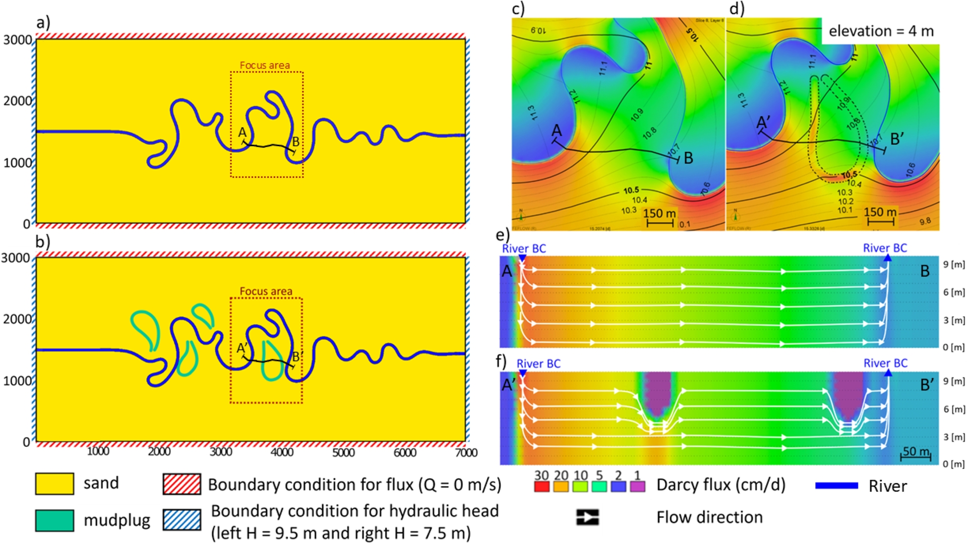
Conventional observations coupled with unconventional data (heat or biogeochemical tracer, geophysical data) allow addressing these limitations of GW modeling (De Marsily, Delay, Gonçalvès, et al., 2005; Schilling et al., 2019; Casillas-Trasvina et al., 2024). Concentration and temperature data are more commonly available and jointly used with the hydraulic head in inversion processes (Ellison et al., 2025). Recent reviews demonstrate the role of geophysics in hydrological studies, for characterizing underground hydrofacies, constraining the GW architecture, and estimating key hydrological properties such as hydrodynamic and thermal parameters (S. S. Hubbard and Rubin, 2000; Parsekian et al., 2015; Binley and Kemna, 2005; Hermans, Goderniaux, et al., 2023; F. M. Wagner and Uhlemann, 2021; Dumont and Singha, 2024). These methods provide spatially extensive, non-invasive insights into subsurface architecture and hydrofacies distributions (S. S. Hubbard and Rubin, 2000; Parsekian et al., 2015; Binley and Kemna, 2005; Hermans, Goderniaux, et al., 2023). Beaujean et al. (2014), Copty et al. (2016), and Irving and Singha (2010) show that integration of geophysics results inside GW models can significantly improve the accuracy of the model compared to using hydrogeological data alone. Common geophysical approaches such as electrical resistivity tomography (ERT), seismic refraction tomography (SRT), and temperature tracer are widely applied in transient states and complex, heterogeneous geological environments at the hillslope scale.
Understanding and modeling shallow groundwater systems in heterogeneous environments remains a major challenge in hydrology and CZ science. This review explores how the integration of geophysical methods, specifically electrical, thermal, and seismic techniques, can enhance our ability to characterize and model these complex systems. We synthesize recent advances, highlight methodological developments, and propose directions for future research at the interface of geophysics and hydrology.
We begin by outlining the fundamental principles and applications of these three geophysical methodologies, highlighting their respective strengths and limitations in the context of heterogeneous shallow GW investigations. A particular focus is placed on the potential of these methods to reveal 4D GW fluxes, which are often poorly constrained in heterogeneous shallow GW. Recent advances in incorporating geophysical data into groundwater models are then discussed, with a particular focus on the development of various inversion approaches that optimize data assimilation and improve model reliability.
Finally, we identify emerging methodological developments and propose key research directions for integrating hydrogeophysical data into GW models, thereby bridging the gap between theory and practice. These include strategies for effective field data monitoring, the development of scalable hydrogeophysical models, and robust approaches for quantifying uncertainty.
2. Geophysical methods, petrophysics, and geostatistics
To identify hydrofacies parameters, common hydrological practices include laboratory measurements, pumping tests (Theis, 1935; Papadopulos and Cooper Jr., 1967; C. E. Jacob and Lohman, 1952; Black and Kipp Jr., 1981), GW time-series analyses, such as data in the spectral domain (Gelhar and Wilson, 1974; Guillaumot et al., 2022; Pedretti et al., 2016; Schuite et al., 2019), or responses to Earth or atmospheric tides (Klönne, 1880; Rau, Cuthbert, et al., 2020; Meinzer, 1939; M. L. Merritt, 2004; McMillan et al., 2019; Thomas et al., 2024; Valois et al., 2024). Critics argue that these methods are inherently local, dependent on the design of pumping test experiments, piezometer placement, and site-specific conditions. There is ongoing debate about the spatial representativeness and upscaling of these parameters from local measurements to hydrogeological models at the hillslope scale. However, these data, combined with detailed geological descriptions, provide valuable constraints for hydrogeological models, improving the calibration and validation of model parameters. These data are commonly used as prior information in hydrogeological modeling, supporting the range of the physical parameter values of the subsurface. Rocks and unconsolidated materials are often described as a mix of various components: rock matrix and multi-fluids (air, water). These characteristics control the physical properties such as the hydraulics, thermal, electrical, and seismic parameters. Therefore, geophysical methods can assist in characterizing hydrofacies through direct modelling and inverse problems solving (Rubin and S. Hubbard, 2005).
2.1. Thermal, electrical, and seismic methods
Equations governing the forward model (FWD) of each method are given in the Appendix B.
2.1.1. Heat as a flow tracer
While temperature is widely acknowledged as a significant state variable with extensive hydrological and hydrochemical impacts, the past decade has seen an increased recognition of the value of temperature measurements to trace subsurface flow paths, especially for GW flow, vadose zone and SW–GW interaction (Anderson, 2005; Kurylyk, Irvine and Bense, 2019; Halloran et al., 2016). Owing to the strong coupling between flow and heat transport, temperature has long been used as a natural tracer to infer subsurface flow processes, beginning with foundational studies in the 1960s (Suzuki, 1960; Stallman, 1965; Bredehoeft and Papaopulos, 1965). In such systems, the advective term in the heat transport equation is directly proportional to specific discharge (Appendices B.1, B.2). The theoretical basis stems from classical heat conduction work by Carslaw and Jaeger (1959) and has been extended to account for advective heat transport under transient conditions (e.g. Campbell et al., 1991; Heitman et al., 2003; Briggs, Lautz, et al., 2012; Simon, Bour, Lavenant, et al., 2021). The increasing availability of affordable temperature sensors facilitates high-resolution monitoring of thermal dynamics in rivers, soil, and aquifers, which provides a natural signal for tracing water movement (Figure 3a, b). Temperature fluctuations, whether diurnal, seasonal, or induced by artificial sources, can be leveraged to infer SW–GW interactions, quantify the GW recharge, delineate subsurface flow paths, and quantify geothermal potential (Hatch et al., 2006; Keery et al., 2007; Kurylyk, Irvine and Bense, 2019; Saar, 2011; Anderson, 2005; Constantz, 2008; Rau, Andersen, et al., 2010; Healy and Cook, 2002).
Using heat as a tracer: (a) Temperature time series recorded in the Orgeval CZ observatory (France) (Tallec et al., 2015; Rivière, Flipo, Ansart, et al., 2018) for aquifer (black line), bank (gray line), and stream (light-grey line) over a decade. (b) Annual temperature regime plot: light blue and red points indicate the daily minimum and maximum temperatures, respectively; the gray-shaded region represents the range between the 0.05 and 0.95 quantiles, and the dark blue line shows the mean. (c) Simulation of a temperature profile as a function of depth for a homogeneous soil, and (d) a heterogeneous soil, for aquifer discharge (orange line) and aquifer recharge (blue line). (c) and (d) showing deviations from the geothermal gradient caused by surface zone and convection in the geothermal zone. Aquifer recharge (downward movement) results in concave upward profiles, whereas aquifer discharge (upward movement) results in convex upward profiles.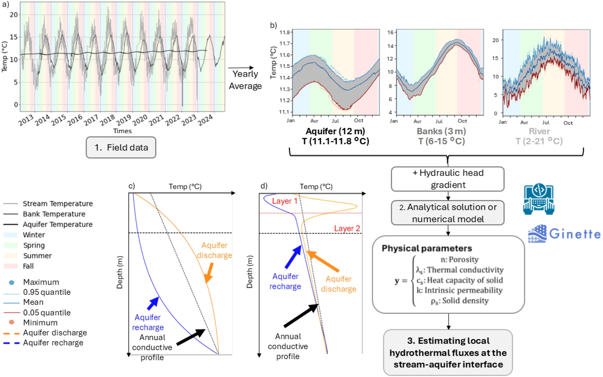
The use of temperature as a hydrological tracer relies on two main strategies: passive and active thermal tracing. Passive approaches take advantage of natural temperature fluctuations, typically diurnal or seasonal surface signals, and analyze their propagation through the subsurface to infer GW flow characteristics (Figure 3a, b). Signal attenuation and phase shifts with depth (Figure 3a) allow estimation of vertical fluxes and thermal diffusivity, particularly in streambeds and in the VZ (e.g. Hatch et al., 2006; Keery et al., 2007; Kurylyk, Irvine and Bense, 2019; Constantz, 2008). Heat is a particularly effective tracer for revealing subsurface heterogeneities, as its transport is highly sensitive to variations in thermal properties and flow paths.
Figure 3c and d present transient temperature profiles produced with the Ginette model (Rivière, Gonçalvès, Jost and Font, 2014; Rivière, Jost, et al., 2019; Rivière, Gonçalvès and Jost, 2020; Grenier et al., 2018), a coupled water- and heat-diffusivity equations, for both homogeneous and two-layer domains, demonstrating the influence of subsurface heterogeneity on heat transfer. During aquifer recharge, surface water infiltrates downward, and advective heat transport produces a concave-upward temperature profile characteristic of downward flow. The infiltrating water may be warmer in summer or cooler in winter, but the curvature remains diagnostic of recharge, while discharge creates a convex or compressed profile near the surface (Figure 3c and d) (Rivière, Flipo, Goblet, et al., 2020). These advective processes stand in clear contrast to purely conductive heat transfer, where temperatures vary only by diffusion and follow a nearly linear trend with depth. In the heterogeneous model, the presence of a shallow, permeable layer accelerates advective transport during recharge and discharge events. As a result, the thermal profile diverges from the expected recharge pattern and instead bends convex-upward. Kurylyk, Irvine, Carey, et al. (2017) demonstrates that heat can serve as an effective hydrologic tracer in both shallow and deep heterogeneous media, offering analytical tools based on the work of Shan and Bodvarsson (2004) and field data to improve subsurface flow characterization. Thermal tracing is widely used to assess SW–GW interactions, as reviewed by Anderson (2005), Saar (2011), and Kurylyk, Irvine and Bense (2019). However, its accuracy relies on having enough advective heat transfer. Recommended intrinsic permeability values range from 10−13 to 10−10 m2 (Cucchi et al., 2021; Smith and Chapman, 1983; Rivière, Flipo, Goblet, et al., 2020). If the conductivity falls below this range, it is not possible to infer intrinsic permeability from thermal data, as heat transport is dominated by conduction.
In the VZ, temperature data have also been used to estimate recharge rates (e.g. Tabbagh, Bendjoudi, et al., 1999; Benderitter, B. Roy, et al., 1993; Bechkit et al., 2014; Halloran et al., 2016). However, inversion under unsaturated conditions requires a fully coupled thermo-hydraulic framework, involving soil-specific relationships for thermal conductivity and water retention (e.g. Van Genuchten, 1980; Mualem, 1976; Brooks and Corey, 1966; Fredlund, 2006). However, no single model yet exists for thermal conductivity in VZ (Cosenza et al., 2003). Thus, testing and comparison with other methods under a variety of conditions, such as low saturation, high saturation, and active infiltration at various rates, is an obvious next step to improve the VZ heat tracer methodology (Halloran et al., 2016). Quantifying vertical GW discharge fluxes necessitates measurement approaches with spatial resolutions consistent with the scale of subsurface heterogeneity and the gradients driving vertical flow (Tabbagh, Bendjoudi, et al., 1999).
Recent advances in measurement technologies have significantly expanded the use of thermal methods to characterize GW flow and heterogeneity. Fiber-optic distributed temperature sensing (FO-DTS) enables high-frequency, high-resolution temperature measurements over long spatial domains (e.g. Tyler et al., 2009; Hermans, Nguyen, Robert, et al., 2014). Applications include resolving small-scale hydrofacies variability and preferential flow paths in alluvial systems. In active FO-DTS, heat is applied along the fiber, and temperature changes are used to infer thermal and hydraulic properties through the inversion. This method has proven particularly effective in high-flux environments, where passive signals may be obscured. Briggs, Lautz, et al. (2012) and Simon, Bour, Lavenant, et al. (2021) demonstrated how thermal signals correlate with known hydrofacies and enhance resolution of vertical water fluxes in the context of SW–GW exchanges.
Drone-based thermal infrared imaging provides complementary surface temperature data across broad spatial extents. In Arctic catchments and braided river systems, UAV-mounted TIR cameras have been used to detect GW discharge zones and identify ecologically significant thermal habitats (e.g. Hare et al., 2016). These systems have been validated against FO-DTS and in-situ sensors, providing an effective platform for regional thermal mapping.
Active thermal tracing offers a controlled approach to investigating subsurface flow by introducing a heat source, via heated probes, injected water, or fiber-optic cables surrounded by a wire acting as a resistance that can heat the medium, and monitoring its spatial and temporal propagation. This approach is advantageous where natural thermal gradients are insufficient to resolve flow dynamics. Moreover, imposing a well-defined heat source significantly reduces uncertainties related to external forcing and simplifies the inversion process. For instance, studies using actively heated DTS have demonstrated the ability to estimate SW–GW exchanges (Briggs, Buckley, et al., 2016; Simon, Bour, Faucheux, et al., 2022). Analytical solutions, such as the moving instantaneous line source model, can then be applied to derive thermal conductivity and SW–GW fluxes with relatively low uncertainty (Simon, Bour, Lavenant, et al., 2021; Simon, Bour, Faucheux, et al., 2022). Similarly, thermal response tests using actively heated fiber-optic cables in boreholes have led to precise estimation of GW flow rates and the characterization of borehole properties by modeling heat transfer in a controlled environment (B. Zhang et al., 2023). Chang et al. (2024) applied this approach for characterizing subsurface heterogeneity and flow dynamics in a tidal-influenced coastal aquifer. The thermal tracer needs to be used for a long period of time, depending on the thermal delay effect (Palmer et al., 1992). Passive temperature sensing might be better for long-term and wide-ranging monitoring (Furlanetto et al., 2024).
Thermal methods offer distinct advantages for studying flow in heterogeneous media (Figure 3c, d). Unlike hydraulic head or solute concentration data, temperature signals can directly characterize the direction, magnitude, and timing of flow across hydrofacies boundaries. However, the nature of heterogeneity, involving abrupt changes in lithology, porosity, hydraulic conductivity, thermal conductivity, and water retention properties, poses different challenges when interpreting heat transport in subsurface systems. Hydraulic conductivity can vary dramatically, which complicates the estimation of GW flow rates based solely on temperature measurements (Constantz, 2008). This necessitates the integration of temperature observations with hydraulic gradient measurements for robust flow characterization (Cucchi et al., 2021).
Joint heat and solute tracer experiments have been proposed to reduce uncertainties in transport predictions by exploiting their complementary behaviors, offering a more comprehensive understanding of subsurface heterogeneity and improving model accuracy (Hoffmann et al., 2019). However, complex three-dimensional flow fields can still introduce significant errors in the estimation of thermal fluxes and effective thermal diffusivity, underlining the need for modeling approaches that explicitly consider spatial variability and flow directionality (Sommer et al., 2013; Reeves and Hatch, 2016).
2.1.2. Electrical resistivity tomography
The electrical conductivity (or resistivity) of geological materials is governed by the lithological properties of the rock matrix, as well as the chemistry, volume, and temperature of internal fluids (Hayley, Bentley, Gharibi and Nightingale, 2007). Consequently, electrical investigation methods provide a direct window into these subsurface parameters. ERT is a preferred near-surface geophysical technique, valued for its non-invasive nature and ease of implementation (Everett, 2013). Its widespread adoption is further supported by various robust data processing software packages (see Appendix B.3) (Loke and Barker, 1996; Blanchy et al., 2020; Rucker et al., 2017). As illustrated in Figure 4, the typical ERT workflow follows three stages: (i) installing electrodes at the ground surface or within boreholes, (ii) collecting apparent resistivity (𝜌a) data using a variety of quadrupole configurations, and (iii) solving an inverse problem to generate a final electrical resistivity model of the subsurface.
ERT method consisting of apparent resistivity measurements during a field survey, data processing or inversion, and interpretation phase. Streamlines and depth of investigation (blue circle) for a given quadrupole ABMN are shown.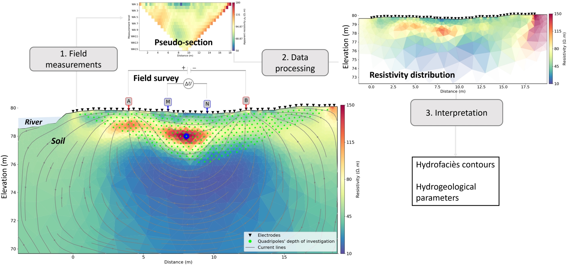
ERT consists in inducing an electrical current (I) in the ground using two injection electrodes (Figure 4). The resulting voltage difference (ΔU) is measured by two potential electrodes. These four electrodes form a quadrupole. The apparent resistivity 𝜌a is then derived from the current, the voltage difference, and the geometrical factor, which depends on the arrangement of the quadrupole’s electrodes. The apparent resistivity represents an average value of the subsurface, assuming a homogeneous half-space. Increasing the spacing between the electrodes allows sounding deeper, but the resulting value remains an integration over the entire volume of ground between the injection electrodes. All quadrupoles of a profile are characterized by a theoretical depth of investigation defined by A. Roy and Apparao (1971) and Barker (1989). A 2D distribution of 𝜌a along a transect can be obtained by combining several combinations of “single” measurements.
Measured apparent resistivity values are then processed and inverted to eventually obtain a resistivity model. This model can be interpreted in terms of subsurface structure (Guérin et al., 2009; Boura et al., 2024), lithology (Guerin et al., 2004; Bentley and Gharibi, 2004), water content, (Tabbagh, Benderitter, et al., 2002; Tabbagh, Bendjoudi, et al., 1999; Bai et al., 2021), hydraulic conductivity (Rehfeldt et al., 1992), salt content (Hayley, Bentley and Gharibi, 2009), transport parameters of tracer plumes (Lekmine et al., 2017; Benderitter and Tabbagh, 1982; Giordano et al., 2017; Hermans, Nguyen, Robert, et al., 2014), or water level (Bentley and Trenholm, 2002; Wu et al., 2023). Inferring parameters from geological and hydrofacies features is possible using petrophysical models from the literature or site-specific information (Section 2.2). For dynamic parameters or variables, a time-lapse approach is required (cf. Section 3.3). Data errors significantly impact both the inversion stability and the subsequent interpretation of the resulting resistivity images (Tso, Kuras, Wilkinson, et al., 2017; Tso, Kuras and Binley, 2019). Often, field data errors are estimated by stacked or reciprocal measurements performed with the resistivity meter (Tso, Kuras, Wilkinson, et al., 2017; Tso, Kuras and Binley, 2019; Dahlin, 2000; Wilkinson, Loke, et al., 2012). Error estimation is essential in the inversion process because underestimating error levels can result in model overfitting, while overestimating them can lead to underfitting, both of which complicate the interpretation of results. ERT output models are particularly challenging to interpret due to the unconstrained nature of ERT images, which are affected by survey configuration, field conditions, subsurface heterogeneity, and the inherent non-uniqueness of the inversion solution. Some tools, such as the PyMERRY code (Gautier et al., 2024), can be employed to quantify uncertainties in ERT images in addition to classical sensitivity computation (Loke, 2004).
2.1.3. Active seismic methods
Seismic approaches are widely employed at various scales in hydrogeology; however, they primarily focus on delineating subsurface contrasts rather than specifying the associated physical properties (Pride, 2005; S. S. Hubbard and Linde, 2011). Seismic reflection can provide high-resolution images of the CZ architecture (Haeni, 1986; Bradford and Sawyer, 2002; Kaiser et al., 2009), but its application in shallow GW is difficult. Gradual weathering often leads to subtle or absent impedance contrasts, hindering strong reflections. Besides, the near-surface exhibits significant heterogeneity, noise, and the presence of surface wave hiding reflection, necessitating dense acquisition and advanced processing for effective imaging. SRT has been increasingly employed in CZ exploration in the last decade (Olona et al., 2010; Befus et al., 2011; Fabien-Ouellet and Fortier, 2014; W. S. Holbrook, Riebe, et al., 2014; St. Clair et al., 2015; Pasquet, Bodet, Longuevergne, et al., 2015; Flinchum, S. W. Holbrook, et al., 2018; Callahan et al., 2020; Cosans et al., 2024), using the inferred pressure-wave (P) velocity (VP) as a proxy to delineate subsurface layers (e.g. soil, regolith, bedrock). Borehole data are used with these images to assign hydrofacies characteristics (Befus et al., 2011; Cassidy et al., 2014; W. S. Holbrook, Marcon, et al., 2019; Guérin, 2005; Olona et al., 2010; Paillet, 1995; Lesparre, Pasquet, et al., 2024).
Nowadays, it is widely acknowledged that hydrofacies parameter values (porosity, fluid saturation, and permeability) can influence seismic properties (Pride, 2005). The major theory which links hydrofacies and seismic parameters is poroelasticity proposed by Biot (1956a), Biot (1956b), and Biot (1962) as described in the Appendix B.4. As the S-wave propagates primarily within the solid frame, the behaviors of P-waves and S-waves are partially decoupled in the presence of fluids (Bachrach, Dvorkin, et al., 2000; Bachrach and Mukerji, 2004). This decoupling implies that P-wave velocity (VP) is sensitive to changes in fluid properties, while S-wave velocity (VS) primarily reflects the elastic properties of the solid matrix. Studying both VP and VS offers valuable subsurface information, enabling more accurate hydrofacies characterization, including porosity and fluid content in the VZ (Pasquet, Bodet, Dhemaied, et al., 2015; Pasquet, Bodet, Longuevergne, et al., 2015) and the piezometric surface (Flinchum, Banks, et al., 2020; Dangeard, Rivière, et al., 2021).
While both VP and VS can be jointly estimated through SRT (Turesson, 2007; Grelle and Guadagno, 2009; Pasquet, Bodet, Longuevergne, et al., 2015), obtaining reliable VS estimates from SRT often presents critical challenges. These include the need for specific sources and horizontal geophone arrays, which increases field effort, and the difficulty in accurately identifying S-wave first arrivals during data processing. To overcome these challenges, VS characteristics are frequently inferred from surface-wave dispersion inversion (L. V. Socco and Strobbia, 2004; L. V. Socco, Jongmans, et al., 2010) (referred to as Multichannel Analysis of Surface Waves, MASW). Recent studies have extensively developed integrated approaches combining SRT and MASW to simultaneously estimate 2D VP and VS sections along coincident profiles from single datasets (Konstantaki et al., 2013; Flinchum, Banks, et al., 2020; Pasquet, Bodet, Dhemaied, et al., 2015; Pasquet, Bodet, Longuevergne, et al., 2015; Pasquet, W. S. Holbrook, et al., 2016). With this approach, seismic methods have become a promising imaging tool for both hydrofacies heterogeneities and water content contrasts through the VP/VS or Poisson’s ratio (𝜐) (Figure 5d). This approach, relying on the open-source processing tools SWIP (Pasquet and Bodet, 2017; Pasquet, Wang, et al., 2021) and PyGIMLi (Rucker et al., 2017), appears successful in various hydrogeological contexts and application scales: from the laboratory on partially saturated glass beads (Pasquet, Bodet, Bergamo, et al., 2016), to the field and the catchment scale (Pasquet, Marçais, et al., 2022). This approach has also proved to be a very promising tool for imaging the VZ water content and the water flow paths within the river corridor (Dangeard, Rivière, et al., 2021). In addition, it has been recently shown that simple neural networks can effectively extrapolate 3D water table maps from passive seismic data, using a limited number of piezometric spatial observations (Cunha Teixeira, Bodet, Rivière, Hallier et al., 2025). Reliance on direct piezometric measured data constrains the method’s broader applicability. To address this limitation, a Transformer-based language model inspired by neural machine translation and speech recognition architectures has been proposed (Cunha Teixeira, Bodet, Rivière, Solazzi et al., 2025). Designed for deterministic petrophysical inversion, it translates surface-wave dispersion data into detailed textual descriptions of subsurface properties, including soil composition, geomechanical parameters, and hydrogeological conditions (basically hydrofacies). This method limits the need for piezometric data and processes seismic data 2000 times faster than conventional stochastic inversion methods, describing both water levels and medium heterogeneities.
Schematic illustration from Solazzi et al. (2021) and Dangeard, Rivière, et al. (2021) of (a) a saturation-depth profile calculated with the Van Genuchten (1980) relationship, (b) associated porous media density 𝜌pm(z,Sw), P-wave velocity Vp(z,Sw), and S-wave velocity Vs(z,Sw) profiles, and (c) body (P and S) and surface (PSV) waves propagating in the partially saturated soil. (d) Sections of Poisson’s ratio (𝜐) estimated from seismic data for each time step and estimated piezometric surface (colored lines). The highest values of 𝜐 indicate a saturated medium, while low values correspond to a partially or unsaturated medium The white shaded area indicates the unconstrained area below the depth of investigation.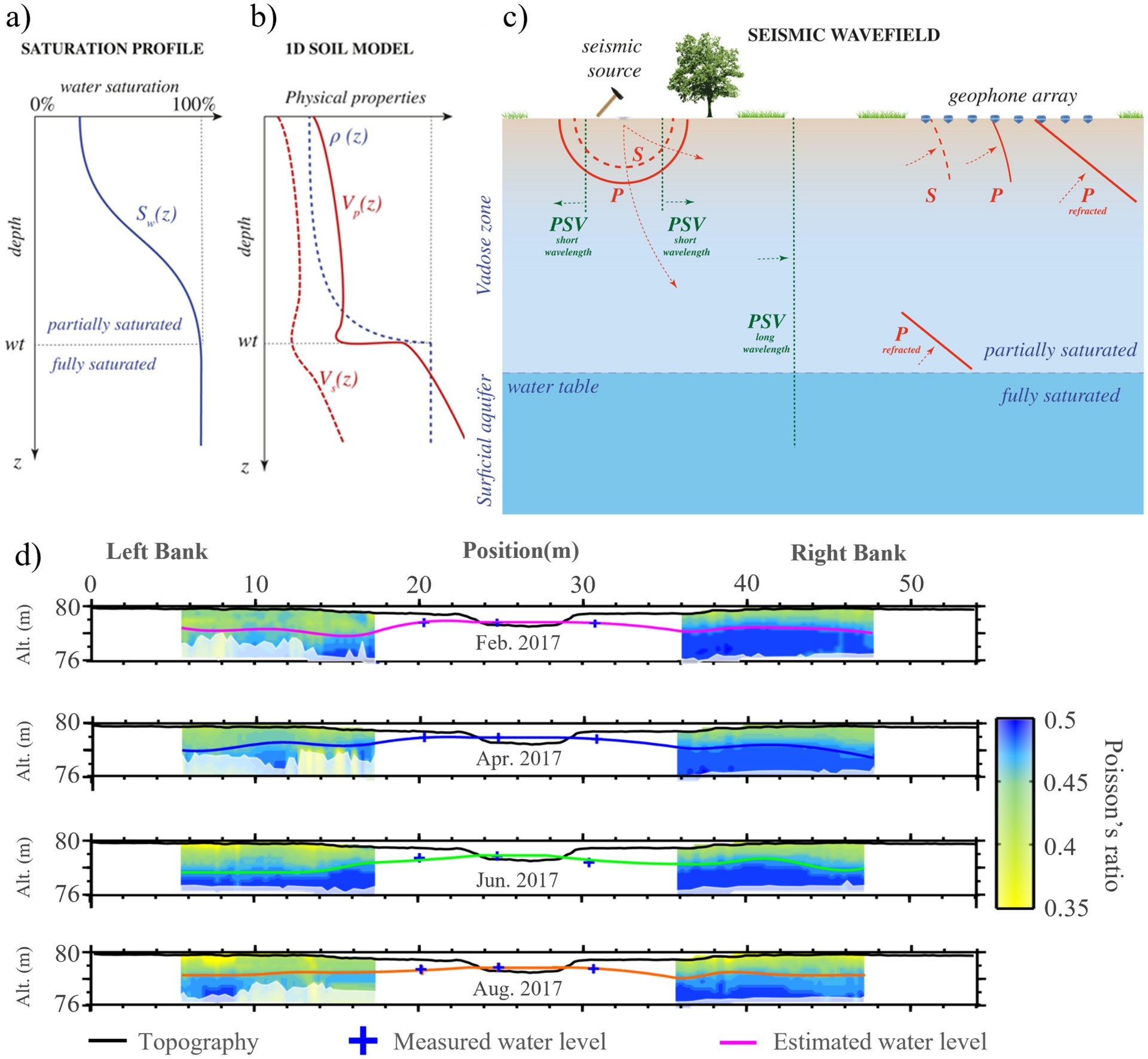
A primary drawback of SRT and MASW is the manual effort required for first-arrival picking and dispersion curve extraction. Furthermore, quantifying the uncertainties associated with these picks remains an active area of research (Dangeard, Bodet, et al., 2018). Errors are controlled by several factors like instrument responses, poor coupling between sources and geophones, tilt angles, near-field offset effects, waveform changes, signal attenuation, and ambient noise sensitivity. Data may not be reproduced accurately due to differences in source frequency or temporal shape from location to location. Automatic source generation cannot guarantee reproducibility in orientation, frequency content, amplitude, and first P-arrival waveforms. These issues are not discussed in the literature.
In recent advanced works in near-surface geophysics, the time-picking process is generally done randomly many times (from 15 to 30 times) by hand for each seismogram, a minimum of 15 times being necessary (Dangeard, Bodet, et al., 2018; Dangeard, Rivière, et al., 2021). A standard deviation is then estimated to quantify the picking uncertainty. Recent deep-learning methods offer more competitive accuracy and speed in time arrival labels compared to classical methods. Transfer and hybrid semi-supervised deep-learning picking approaches can achieve similar accuracies over ten times faster, especially in active seismics (Huynh et al., 2023). This approach is based on PhaseNet, a U-net-based deep learning algorithm initially developed for seismic wave picking (W. Zhu and Beroza, 2019), is improved via Machine-Learning based corrections and extended to the context of active seismic data.
Relative errors of approximately 5 up to 7% are generally obtained for P-wave first arrival for different setup configurations that are very similar at near-surface scales (Pasquet, Bodet, Dhemaied, et al., 2015; Pasquet, Bodet, Longuevergne, et al., 2015; Bergamo and L. Socco, 2016) or at laboratory scales (Bodet, X. Jacob, et al., 2010; Bodet, Dhemaied, et al., 2014; Pasquet, Bodet, Bergamo, et al., 2016). Besides, in those studies, dispersion curves are also extracted from dispersion diagrams using MASW approaches. Fundamental modes such as Rayleigh wave modes can be detected with relative errors lower than 7–10% by using classic random picking or semi-supervised deep-learning approaches (Dai et al., 2021).
2.2. Petrophysical relationships for linking geophysical observables to hydrofacies
Subsurface lithology inherently governs both hydrogeological and geophysical data. To bridge these fields, petrophysical laws provide quantitative links between hydrogeological properties (e.g. porosity, hydraulic conductivity, water saturation) and geophysical parameters, including seismic velocities and electrical resistivity (Pride, 2005; T. C. Johnson, Versteeg, H. Huang, et al., 2009; J. Chen et al., 2001). These relationships are frequently derived through empirical calibrations based on site-specific observations (Huisman, S. S. Hubbard, et al., 2003; Roth et al., 1990; West et al., 2001).
These models can be refined to incorporate additional variables, such as mineral composition, density, and various geophysical parameters. Petrophysical models often exhibit significant variability across different lithologies as they are highly sensitive to fluctuations in mineral composition and pore structure (Mavko et al., 2009). Semi-empirical models, which partially integrate the geometrical and physical characteristics of the porous medium, are widely used in practice. The main relationships and petrophysical models used in hydrogeophysics include:
- Archie’s law: this empirical relationship relates the electrical conductivity of a brine-saturated rock to its porosity and water saturation (Archie, 1942). Numerous studies have adapted this law to their geological context as it is synthesized in Glover (2017), Glover (2015), and Zinszner and Pellerin (2007). For example, Waxman and Smits (1968) and D. L. Johnson et al. (1986) have extended this law to account for surface conduction in the presence of clay, which is particularly important in low-salinity environments.
- Gassmann’s model predicts the impact of fluid saturation on the elastic properties of rocks. It is particularly useful for the seismic approaches (Gassmann, 1951).
- Various petrophysical models and empirical relationships are used in seismic modeling (Schmitt, 2015). For instance, Gardner’s equation is an empirical relationship linking rock density to seismic velocity (Gardner et al., 1974) at the near surface scale. Hertz–Mindlin grain contact theory provides a framework for predicting seismic velocities (VP and VS) based on grain interactions, considering factors like porosity, mineralogy, and fluid saturation (Mindlin, 1949). This model was used to the VZ by Solazzi et al. (2021). The Kuster–Toksöz model predicts the elastic properties of randomly oriented pores in rocks, particularly in establishing relationships between lithofacies parameters with seismic velocities (Mavko et al., 2009; Kuster and Toksöz, 1974). Additionally, the relationship of N. I. Christensen and Stanley (2003) correlates porous media density to VP and VS.
- The empirical Kozeny–Carman relationship relates hydraulic conductivity to porosity and specific surface area (Wyllie and Rose, 1950; Carman, 1937; Kozeny, 1927).
These petrophysical models have been empirically adapted for CZ applications to characterize soil water content (Pasquet, Marçais, et al., 2022; Gase et al., 2018; A. J. Merritt et al., 2016; Pasquet, W. S. Holbrook, et al., 2016; A. P. Tran et al., 2014), porosity distribution (Mezquita Gonzalez et al., 2021; Callahan et al., 2020; Flinchum, W. S. Holbrook, et al., 2018; W. S. Holbrook, Riebe, et al., 2014; Mount et al., 2014), hydraulic conductivity (Di Maio et al., 2015), and fluid content (Yuan et al., 2023; Holmes et al., 2022). Petrophysical models can be derived from both laboratory measurements (e.g., core and plug analyses, well logs) and geophysical inversions. Laboratory data provide direct, high-resolution measurements at the core scale (Schön, 2015), although the samples may not fully represent in-situ conditions because their properties can be altered during coring, extraction, and transport. Geophysical inversions yield indirect, spatially regularized estimates that integrate over larger volumes and depend on prior assumptions and inversion constraints (Tarantola, 2005; Aster et al., 2018). Both sources are widely used and typically complement each other in subsurface characterization (Pride, 2005; Linde and Doetsch, 2016).
A key challenge arises when applying petrophysical laws to these geophysical inverted fields. Geophysical inversions produce spatially correlated models due to both the physics of data acquisition and the regularization applied during inversion. Typically, these fields exhibit long-range continuity in the horizontal direction and short-range continuity in the vertical direction, reflecting geological layering and the geometry of surface measurements (Chilès and Delfiner, 2012; Isaaks and Srivastava, 1989; Grana et al., 2022). In addition, poorly constrained petrophysical relationships themselves remain a major source of uncertainties in models (e.g. Seo et al., 2025; Tso, Kuras and Binley, 2019; Brunetti and Linde, 2018).
2.3. Geostatistical methods for subsurface characterization
Integrating diverse data types requires the application of robust geostatistical algorithms. While high-resolution spatial studies often rely on datasets with limited 2D extent, there is a growing need to incorporate 3D or 4D (timelapse) dimensions. To address these complexities, several powerful geostatistical frameworks are available. The package gstlearn (D. Renard, Ors, et al., 2025), developed by Mines Paris, offers a comprehensive suite of tools for such multivariate challenges, complementing other established packages like geoR (Ribeiro Jr. and Peter, 2025), gstat (Pebesma and Wesseling, 1998), or GEONE (DeeSse) (Zhexenbayeva et al., 2024). A key challenge is to construct a three-dimensional model providing the hydrofacies distribution by assigning probabilities to the geophysical property values associated with a particular medium (Gottschalk et al., 2017; L. Zhu et al., 2016).
Hard data, or quantitative data, refers to information that is measurable and verifiable. It is a type of data that is measured and can be analyzed statistically. In contrast, soft data and qualitative data are mostly derived indirectly (for example, related to the variable of interest), are usually more numerous and less accurate than hard data because of their indirect nature. One, two, or three-dimensional spatial information derived from geophysical imaging and hydrogeological interpretation (e.g. cross-sections or calibrated flow models) are inherently uncertain and therefore considered as soft data. Combined with geological logs (hard data), they could be used to perform conditional geostatistical simulations.
Ordinary kriging has also been applied in critical zone studies to interpolate CZ architecture, as demonstrated by a 3-D seismic velocity model constructed beneath a soil-mantled granite ridge in the Laramie Range, Wyoming, using 25 seismic refraction transects (Flinchum, S. W. Holbrook, et al., 2018). This geostatistical approach enabled the delineation of subsurface layers and improved understanding of deep CZ structure. Similar kriging-based strategies have been implemented to map critical zone compartment geometry, such as in the Strengbach watershed (Vosges Mountains, France) (Lesparre, Pasquet, et al., 2024), and in the Quiock watershed (Guadeloupe archipelago, France) (Pasquet, Marçais, et al., 2022).
The multiple-point simulation (MPS) approach developed by Strebelle (2002) can be used to provide simulated facies maps. In practice, it directly uses empirical distributions inferred from one or several training images that can be derived either from similar outcrop observations, expert knowledge, or geophysical data (Caers et al., 2003; Linde, P. Renard, et al., 2015). Among the MPS methods, Direct Sampling is often employed since it is very flexible and computationally efficient (Meerschman et al., 2013). It has been recently extended for the simulation of multi-resolution patterns (Straubhaar, P. Renard and Chugunova, 2020), or for handling complex conditioning data such as inequality constraints (Straubhaar and P. Renard, 2021). These methods reproduce complex geometries such as channels, meanders, or lenses while preserving the relations between the facies.
An alternative is the Plurigaussian Geostatistical Simulation (PGS) approach. PGS has long been acknowledged as a practical tool for assessing the impact of subsurface heterogeneity on field and basin scale flow and transport processes (Armstrong et al., 2011; Le Loc’h et al., 1994; Abzalov and D. Renard, 2023). The outcome of MPS and PGS simulation methods is a set of 3-D equiprobable realizations of hydrofacies that are conditioned by the hard data and can be used to derive the probability of occurrence for each hydrofacies at a given location.
Process-based or hybrid stochastic/genetic models, such as Flumy, can be employed to generate geologically consistent prior realizations. These models more faithfully capture sedimentary dynamics while remaining strongly conditionable to geophysical and hydrological data. In this way, Flumy-type priors can complement geostatistical interpolation by providing more realistic subsurface structures that serve as a robust basis for hydrogeophysical inversion across different dimensionalities (1D–3D). Moreover, Hermans, Nguyen and Caers (2015) demonstrated how training-image-based priors can be updated or falsified using electrical resistivity tomography (ERT) data, improving the consistency between geological scenarios and geophysical observations. Building on this, Neven, Schorpp, et al. (2022) introduced a multi-fidelity inversion framework that combines low-fidelity geologically consistent stochastic models with high-fidelity GW flow simulations, enabling efficient joint inversion that preserves geological realism while reducing computational cost.
While such methods are suitable for the simulation of heterogeneous media, the addition of geophysical and hydrological data (secondary information) makes them potentially more powerful. Bayesian sequential simulation method (BSS) from Doyen and Den Boer (1996) provides an attractive alternative for simulating jointly primary and secondary variables, without requiring any linear or specific parametric relationship between the variables. The method is based on PGS, with the addition that the conditional distribution estimated by kriging is updated by the joint distribution of the primary and secondary variables in a Bayesian framework. While BSS is recognized as a powerful and flexible geostatistical tool (J. Chen et al., 2001; Chilès and Desassis, 2018), it also provides significant improvements. In particular, the simultaneous reproduction of: (i) the variance and the fine-scale structure, and (ii) the relationship between the primary and the secondary variables. It is particularly adapted for the hydrogeophysical applications, in order to deal with the smooth behavior of the secondary variable due to the regularization procedure involved in the geophysical inversion procedures.
The traditional geostatistical framework assumes that the spatial characteristics of the variables are defined and valid over the whole field. It fails at reproducing local changes. For that sake, the new branch of non-stationary Geostatistics has been recently launched which offers the possibility to consider any parameter of the spatial characteristics (e.g. range, anisotropy orientation, variogram sill) as defined locally (D. Renard, Ors, et al., 2025). To be fruitful, this technique requires additional information such as a proxy driving the anisotropy orientation (following a meander direction for example) or a proxy for the variance (following the river flow for example) (Fouedjio, 2014).
3. Geophysical and hydrological wedding
Historically, a disciplinary divide has persisted between geophysicists and hydrogeologists, largely driven by diverging research priorities. While geophysicists have traditionally focused on advancing instrumentation, inversion algorithms, and interpretation frameworks, hydrogeologists are deeply driven by the development of predictive models to simulate complex hydrological processes within the CZ. This disconnect often arises from a difference in application: hydrogeologists frequently seek to optimize their numerical models using geophysical data as a spatial constraint, whereas geophysicists have historically prioritized the methodological validation of the signal itself over the broader hydrological outcomes (Robinson et al., 2008). The emerging fields of hydrogeophysics (Binley, S. S. Hubbard, et al., 2015) and CZ sciences aim to bridge the gap between geophysical and hydrological data to explore their interrelationships. Both disciplines seek to understand subsurface processes using the same Laplace’s equations. Researchers are increasingly focused on correlating equation parameters, converting geophysical measurements into hydrological features and vice versa, to develop more precise, data-driven models.
3.1. Conceptual framework for data and model integration
Integration of geophysical and hydrological models requires robust inversion frameworks capable of reconciling sparse and indirect observations with inherent complexity of subsurface dynamics. The inversion process seeks a parameter distribution that minimizes a misfit function (i.e. the discrepancy between observed and synthetic data); in order to identify the physical properties that govern processes such as GW flow or electrical resistivity. In practice, these inversion strategies are generally categorized into deterministic and stochastic approaches.
As illustrated in Figure 6, the methodologies for integrating hydrogeophysical data follow two main workflows: (i) sequential hydrogeophysical inversion (SHI), where data are processed through separate and/or successive stages; (ii) processes based inversion (PBI), which solves for the underlying transient process-based parameters directly (Hellman et al., 2017; Herckenrath et al., 2013; Hinnell et al., 2010; F. M. Wagner and Uhlemann, 2021; F. M. Wagner and Uhlemann, 2021; Linde, Ginsbourger, et al., 2017; S. S. Hubbard and Linde, 2011).
(a) Sequential hydrogeophysical inversion (SHI): geophysical data are independently inverted and interpreted to inform the structural framework of the hydrogeological model, which is then calibrated using hydrological observations. (b) Process-based inversion (PBI): hydrological and geophysical forward models are dynamically linked. Multiple geophysical and/or hydrological datasets are integrated within a unified inversion framework, with coupling terms or petrophysical constraints. Arrows represent the flow of information as well as iterative parameter and condition updating, continuing until a minimum data and/or constraint misfit is achieved.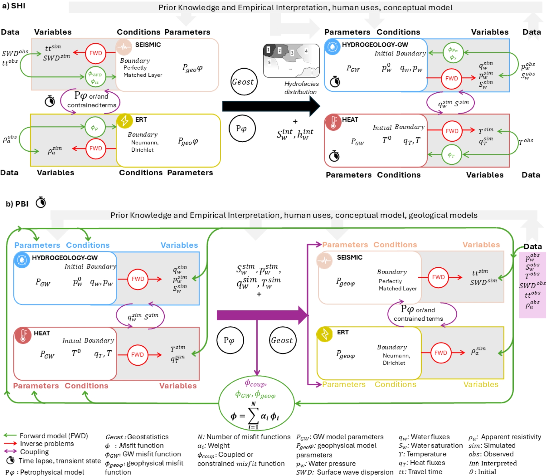
3.1.1. Deterministic inversion: local optimization
Deterministic inversion methods are based on the computation of the gradient of the misfit function using local iterative linearization approaches. In these common local approaches, to reduce the space of possible solutions, a regularization procedure is applied (Menke, 2012) often imposing smoothness or closeness to a prior model. If the initial solution is too far from the global solution, the inversion can be stopped in a local minimum or in an area where the cost function does not significantly change. Linearized approximations like those used by Cockett et al. (2018) remain computationally efficient, but may fail in highly nonlinear or ill-posed settings (Dagasan et al., 2020). Moreover, local approaches are not suitable for estimating reliable uncertainties.
3.1.2. Stochastic inversion and uncertainty quantification
In contrast, stochastic inversion approaches aim to explicitly quantify uncertainty by sampling the posterior distribution of model parameters (e.g. Vrugt et al., 2013; Rings et al., 2010; Hinnell et al., 2010; Y. Chen et al., 2003; Sambridge and Mosegaard, 2002; S. S. Hubbard and Rubin, 2000). Rawlinson et al. (2014) give a comprehensive description of existing methods for estimating uncertainties and illustrate that a posteriori probabilistic distribution sampling of model parameters within a Bayesian framework is much more suitable. As a matter of fact, importance sampling enables the cost function to be sampled proportionally to the probability (Tarantola, 2005). This sampling is generally carried out using Markov chain Monte Carlo (MCMC)-based algorithms (Mosegaard and Tarantola, 1995; Sambridge and Mosegaard, 2002). State-of-the-art inversion (e.g. Aster et al., 2018; H. Zhou et al., 2014; Tarantola, 2005) and data assimilation (e.g., ensemble smoother, ensemble Kalman filers and its variants) (e.g. McAliley et al., 2022; Jiang et al., 2021; X. Chen et al., 2013) are generally used to ingest the hydrological and geophysical data.
3.1.3. Misfits definition
The combination of various misfits related to dynamic data, such as water level or temperature, with those of spatial data, including travel time, water level geometry, or electrical resistivity, is not straightforward. In the sequential hydrogeophysical inversion, the objective functions are estimated independently, whereas in the joint, coupled or process-based inversion, the objective function can assume various forms (Mboh et al., 2012; Hinnell et al., 2010; Rubin and S. S. Hubbard, 2005) (see section below). The misfit of each measurement can be weighted in the objective function according to the measurement uncertainty and sensitivity of each method.
3.2. Static hydrofacies characterization by Sequential hydrogeophysical Inversion approaches (SHI)
In a SHI, geophysical data is separately inverted to estimate the distribution of a single geophysical property (e.g., a map of resistivity). Estimated geophysical property maps are subsequently employed to delineate hydrofacies structures, including the number, geometry, and spatial distribution of facies boundaries of the hydrogeological FWD (Figure 6a) or state variable (e.g., saturation or salinity from resistivity) (Binley, S. S. Hubbard, et al., 2015; Singha, Day-Lewis, et al., 2015; Razafindratsima et al., 2014; Bendjoudi et al., 2002; S. S. Hubbard and Rubin, 2000; Rubin, Mavko, et al., 1992). In these workflows, geophysical and hydrological models are processed sequentially rather than iteratively. The objective functions of the geophysical and hydrological models are not linked; each model is calibrated independently without direct coupling between their respective misfit functions. The geophysical data are first interpreted independently to infer subsurface structure, which then informs the hydrogeological FWD (Figure 6a). After defining the inversion framework, GW flow and transport simulations, whether stochastic or deterministic, are conditioned on prior estimates of hydrofacies parameters such as hydraulic conductivity or porosity. These prior ranges, which help constrain parameter uncertainty, are typically derived from laboratory analyses, pumping tests, or empirical correlations with well-log or geophysical data (Hyndman et al., 1994; Ahmed et al., 1988). In addition to defining prior ranges, certain measurements, such as pumping tests, can also be incorporated directly into the inversion process. The calibration of the GW model parameter is then carried out while keeping the conceptual model fixed (S. J. Kollet and Maxwell, 2006). The earliest study that used this approach was conducted by Ahmed et al. (1988), which used the co-kriging of measured transmissivity, specific capacity, and electrical resistivity to elaborate transmissivity maps.
Geophysical joint inversion involves integrating multiple geophysical data types to improve the characterization of subsurface properties. This approach is particularly beneficial in complex heterogeneous environments (Gallardo and Meju, 2007). To reduce such drawbacks, joint inversion methods combining SRT and ERT simultaneously have been developed at the near-surface scale (Doetsch, Linde, Vogt, et al., 2012; Gallardo and Meju, 2007; Gallardo and Meju, 2004) and could be extended to hydrogeophysics problems. Different constraints linking directly the P and/or S velocities to resistivity, such as petrophysical models, cross-gradients (similarity constraints) can be introduced in the misfit function to reduce the models’ uncertainties during the inversion process. Furthermore, a priori geological information such as lithological boundaries could also be inverted during the inversion process at the same time as the property values or separately by introducing level-set constraints as in Giraud et al. (2021), and Zheglova et al. (2018). Recent studies have adopted multiple-point geostatistics or geological scenario modeling to generate ensembles of plausible hydrofacies configurations (Hermans, Nguyen and Caers, 2015; Neven and P. Renard, 2023). These scenarios are subsequently evaluated by comparing simulated responses with observed geophysical data, often through a probabilistic falsification procedure, providing a more robust basis for structural inference. By extending those approaches to hydrogeophysics, more particularly to seismic data and ERT, it could be possible to reconstruct geological features compatible with different physics but also to retrieve physical properties that are not necessarily correlated. If VP seismic models using ray-tracing-based inversions and VS seismic models using wave dispersion curves inversions can be obtained, they can also be improved by using full waveform inversion at the hydrogeophysical scale (Groos, Schäfer, et al., 2017; Groos, Schafer, et al., 2014; X. Liu et al., 2022). For example, Eppinger et al. (2024) developed a full-waveform tomography workflow to investigate 2D weathering patterns in the critical zone, applied in the Medicine Bow National Forest (USA). Their results are promising, but they also point out that extending the approach to 3D would require substantially greater computational resources.
Besides, joint inversions can be performed using various combinations of physics, such as different heat tracing, ERT, Ground Penetrating Radar, SRT, and MASW, and constrained by petrophysical models relating parameters that characterize the medium under study. Those petrophysical constraints allow not only to reduce the number of free parameters but also to obtain a final inverted model compatible with the different physics (Qin et al., 2024; Steiner et al., 2022; F. M. Wagner and Uhlemann, 2021; F. M. Wagner, Mollaret, et al., 2019).
As long as the inversion is deterministic, a key limitation of geophysical joint inversion approaches is their reliance on multiple geophysical datasets to define a single groundwater conceptual model, which may not fully capture subsurface heterogeneity. In addition, this approach can create discrepancies related to state variables such as water saturation or pressure, and it does not account for the transient behavior of these variables, which is critical in dynamic groundwater systems. If the geometry was fixed before inverting for hydrogeological parameters, and not correctly estimated, the hydrogeological parameters will likely have to be incorrectly identified during inversion in order to compensate for these initial errors (De Marsily, Delay, Teles, et al., 1998). The outputs of GW simulations, such as saturation, hydraulic heads, fluxes, or transport behavior, do not influence the geophysical inversion, while the hydrofacies parameters influence geophysical data. This issue becomes particularly critical under transient conditions, where the dynamic evolution of water and heat fluxes provides valuable information that could help refine both structural and parametric interpretations of the geophysical data. Recent studies have adopted multiple-point geostatistics or geological scenario modeling to generate ensembles of plausible hydrofacies configurations (Hermans, Nguyen and Caers, 2015; Enemark, Peeters, et al., 2019; Enemark, Madsen, et al., 2024).
3.3. Toward transient hydrogeophysical inversions
The CZ requires time-lapse geophysical surveys to move beyond static imaging and effectively monitor and quantify dynamic subsurface processes over time, thus transitioning geophysics from a field primarily concerned with static structural imaging to one adept at monitoring and quantifying dynamic physical and biogeochemical processes. This continuous monitoring has demonstrated efficacy in identifying transient processes in the CZ, such as water infiltration (Daily et al., 1992; Wehrer et al., 2016; R. Hu et al., 2023; Blazevic et al., 2020), variations in water storage (Galibert, 2016), flowpaths identification (Nyquist et al., 2018) GW recharge, and the propagation of thermal fronts (Shariatinik et al., 2024; Lesparre, Robert, et al., 2019; Hermans, Wildemeersch, et al., 2015). The three first methods are based on the SHI approaches.
3.3.1. Absolute inversion
Absolute inversion is the method commonly used to interpret time-lapse datasets. Every geophysical dataset is inverted independently. Transient subsurface changes are then identified by comparing the resulting models for each time step, either on the basis of absolute values or relative differences (Herckenrath et al., 2013; LaBrecque, Morelli, et al., 1995; Daily et al., 1992; Slater et al., 2000). This method is computationally efficient and simple. However, some studies have shown that this approach can result in unrealistic geophysical parameters changes because it is sensitive to data noise and does not directly account for time correlations or hydrological constraints (Miller et al., 2008; Loke, Wilkinson, et al., 2022; T. C. Johnson, Versteeg, Day-Lewis, et al., 2015; LaBrecque and X. Yang, 2001). To address the limitations of absolute inversion, several hydrogeophysical strategies have been developed, as discussed in the following subsections.
3.3.2. Difference inversion
Differencing and ratio methods focus directly on changes between datasets, rather than reconstructing each model separately, allow to decrease these effects (LaBrecque and X. Yang, 2001). The difference inversion enhances sensitivity to temporal changes by inverting differences in data 𝛿dt = dt − d0, and model parameters 𝛿mt = mt − m0, where m0 is the baseline model. The inversion is typically linearized around the baseline using a Jacobian matrix Jij = (∂dt,sim,i)/(∂mt,j) which quantifies the sensitivity. Introduced by LaBrecque, Ramirez, et al. (1996), it can also be computationally efficient if the Jacobian is reused across time steps (LaBrecque and X. Yang, 2001). This approach has proven valuable in resolving subsurface changes with time-lapse ERT during heat-tracing experiments and solute transport, as shown by Hermans, Kemna, et al. (2016) and Bretaudeau et al. (2021), who applied covariance-based constraint of model differences and double-difference inversion schemes to improve sensitivity and reduce artifacts.
3.3.3. Time-constrained inversion
The time-constrained inversion introduces temporal smoothness constraints to stabilize the inversion across time steps. It minimizes a cost function that balances two terms: (i) the data misfit, measuring agreement with the observed responses, and (ii) a temporal regularization term, penalizing abrupt parameter changes over time. The optimization is frequently solved using Gauss–Newton iterations, with the Jacobian matrix Jij = (∂dt,sim,i)/(∂mt,j) quantifying the sensitivity of simulated data to parameter updates.
Several strategies have emerged. Sequential approaches invert each time step independently, using a baseline reference model (typically from the initial survey, t0) to compute resistivity changes at subsequent time steps (Miller et al., 2008). The baseline model (t0) is typically acquired under reference conditions (e.g., before hydrological perturbations) and serves as the structural and resistivity reference for all subsequent surveys. In this framework, each survey is inverted separately, and time-lapse changes are analyzed by comparing the inverted models post-inversion. While computationally efficient, this approach can introduce noise amplification and inconsistencies between surveys, as each inversion is subject to different regularization choices and data quality variations, which can lead to anomalous artifacts (Lesparre, Robert, et al., 2019).
In contrast, joint inversion frameworks have been proposed, in which all time steps are inverted simultaneously while imposing temporal smoothness constraints (Kim et al., 2013; Karaoulis, Tsourlos, et al., 2014; Wilkinson, J. E. Chambers, et al., 2022; W. Zhou et al., 2025; Karaoulis, Revil, et al., 2013; Doetsch, Linde and Binley, 2010). These methods improve model stability and reduce artifacts in dynamic environments like riverbeds (McLachlan et al., 2020), during solute transport (Karaoulis, Tsourlos, et al., 2014). However, excessive smoothing may obscure real changes, and coarse inversion meshes may limit resolution (B. Liu et al., 2020; Hermans, Wildemeersch, et al., 2015).
One promising strategy is to embed geostatistical information that characterizes the spatial correlation structure of the subsurface. For example, in an alluvial context, Jordi et al. (2018) constructs regularization operators based on an exponential covariance model that describe the heterogeneities of the subsurface. Applications of this approach to layered alluvial systems are demonstrated by Palacios et al. (2020) and Arboleda-Zapata et al. (2025).
3.3.4. Transient process-based inversion: joint inversion or fully coupled hydrogeophysical inversion
Process-based hydrogeophysical inversion refers to approaches that dynamically couple hydrological and geophysical FWDs, enabling simultaneous data integration and bidirectional interaction during the inversion process. In time-lapse applications, these methods incorporate temporal evolution of subsurface parameters and state variables (Hermans, Goderniaux, et al., 2023). The hydrogeophysical literature uses various terms, including “coupled hydrogeophysical inversion”, “joint hydrogeophysical inversion”, “process-based inversion” (F. M. Wagner and Uhlemann, 2021), and “fully-coupled inversion” (S. S. Hubbard and Linde, 2011), often interchangeably to describe approaches that integrate hydrological and geophysical data (Linde and Doetsch, 2016; Finsterle and Kowalsky, 2008). While terminology varies across the community, these approaches share the common goal of coupling hydrological and geophysical models through petrophysical relationships to avoid the biases inherent in sequential approaches (Day-Lewis et al., 2005; Linde and Doetsch, 2016; Herckenrath et al., 2013). The key differences lie in implementation strategies—specifically, how petrophysical relationships are incorporated into the inversion framework—rather than in formal nomenclature.
In one common implementation (often termed coupled hydrogeophysical inversion), the hydrological FWD provides state variables such as water saturation, salinity, or temperature, which are converted into geophysical parameter distributions through petrophysical models (Figure 6b) (S. S. Hubbard and Linde, 2011; Huisman, Rings, et al., 2010; Linde and Doetsch, 2016; F. M. Wagner and Uhlemann, 2021; Bascur and Yañez, 2025). The parameters of the hydrological FWD are updated by minimizing a combined objective function that accounts for both hydrological and geophysical misfits (Mboh et al., 2012; Hinnell et al., 2010). A key advantage is that geophysical inversion is guided by hydrological process models, with petrophysical-hydrological regularization avoiding the potential biases arising from traditional geophysical regularization, such as smoothness and smallness constraints (Day-Lewis et al., 2005; Linde and Doetsch, 2016).
An alternative implementation strategy (often termed joint hydrogeophysical inversion) processes multiple datasets simultaneously, enforcing structural or petrophysical consistency across geophysical and hydrological FWDs (Figure 6c) (Herckenrath et al., 2013; Steklova and Haber, 2017). This approach employs a modular framework that integrates the parameters of hydrological and geophysical models into a unified vector. The inversion process minimizes an integrated objective function comprising three weighted components: geophysical data misfit terms (ΦSWD, ΦTT, Φ𝜌), hydrogeological data misfit terms (Φpw, ΦSw, ΦT), and an explicit coupling constraint misfit (Φcoup). The most common coupling mechanisms are petrophysical relationships (F. M. Wagner and Uhlemann, 2021; Steklova and Haber, 2017). This strategy differs from the previous approach in that both hydrological and geophysical parameters are simultaneously estimated, with petrophysical relationships serving as explicit constraints rather than forward transformations.
A critical challenge in both approaches is the appropriate weighting of different misfit terms to balance the influence of diverse data types with varying units, sensitivities, and uncertainties (Linde and Doetsch, 2016). Common approaches include equal weighting of normalized misfits, uncertainty-based weighting (where weights are inversely proportional to data variance or covariance matrices), and data error-based weighting (Mboh et al., 2012; Kowalsky et al., 2006; Linde and Doetsch, 2016). Mboh et al. (2012) demonstrated that uncertainty-based weighting using the inverse of data covariance matrices provides a statistically rigorous framework for balancing electrical resistance and hydrological measurements in coupled inversion. N. K. Christensen et al. (2016) showed that propagating geophysical data uncertainties into hydrological model calibration significantly affects prediction error, highlighting the importance of proper error-based weighting strategies. More sophisticated strategies have emerged, including: (i) adaptive weighting schemes that adjust weights during the inversion process (Steklova and Haber, 2017), (ii) ensemble-based data assimilation approaches where weighting is handled through estimated data-model covariances rather than fixed scalar weights (Neven and P. Renard, 2023), (iii) multi-objective Pareto optimization that avoids pre-selecting scalar weights by producing trade-off solution fronts (Danek et al., 2019), (iv) Bayesian frameworks where weights naturally emerge from data and prior covariance matrices (Dettmer et al., 2024). However, weight selection remains partly subjective and can significantly influence inversion results, particularly when data quality or petrophysical uncertainty varies across datasets (Commer et al., 2013; Finsterle, Commer, et al., 2017).
In alluvial aquifer settings, Herckenrath et al. (2013) demonstrated that this approach improves parameter estimation and model consistency compared to sequential hydrogeophysical inversion when high-quality petrophysical constraints are available, though at a higher computational cost. Recent applications highlight both the opportunities and challenges of hydrogeophysical inversion. For example, Pleasants, Neves, et al. (2022), Pleasants, Kelleners, et al. (2023) and Boyd et al. (2024) used time-lapse ERT data in mountainous regions to improve groundwater flow models. In these studies, simulated water saturation was first converted to resistivity using petrophysical relationships (e.g., Archie’s Law). A weighted misfit function was then employed to compare these modeled resistivities with ERT data and to balance the influence of the different data types during calibration. Bascur and Yañez (2025) introduced a Hybrid Bayesian Inversion framework for CHI using single-time 2-D ERT data from an unconfined alluvial aquifer. Their approach jointly integrates saturated GW FWD modeling with geophysical observations via uncalibrated petrophysical models, with weighting naturally emerging from the Bayesian framework through data and prior covariance matrices. Tested on both synthetic and experimental datasets, this framework provides efficient uncertainty quantification and is particularly suited to estimating water fluxes in heterogeneous aquifers. To address computational challenges, Neven, Schorpp, et al. (2022) proposed a stochastic multi-fidelity framework integrating Ensemble Smoother with Multiple Data Assimilation (ES-MDA) and multi-fidelity modeling. Applied to both synthetic and real datasets, this approach improved accuracy while significantly reducing computational costs.
The recent development of a fully coupled GW–ERT FWD using pore water pressure as the coupling variable (Salas-Ariza et al., 2025) represents a promising methodological advancement. A sensitivity analysis of this model was performed, though full inversion using the coupled framework in real field applications had not yet been demonstrated at the time of publication.
Both implementation strategies are typically applied to sites with relatively simple geometries, low heterogeneity, and limited multiphysical calibration datasets. Future research is needed to address the definition of coupling terms between different FWDs, the assignment of weights in objective functions for various data types, and the evaluation and quantification of petrophysical uncertainty. While coupled hydrogeophysical inversion has demonstrated success in controlled settings and moderately complex field sites, extending these approaches to highly heterogeneous systems with complex geometries remains challenging.
4. Remaining challenges and future directions
Shallow groundwater processes in the critical zone occur within strongly heterogeneous environments, where heat, water, and solute fluxes vary in space and time (Huggins et al., 2023). Surface interfaces such as SW–GW boundaries and the vadose zone are especially heterogeneous (see Appendix A), making it difficult to resolve the associated four-dimensional water and heat fluxes. Despite recent advances in hydrogeophysics and modeling, accurately characterizing and predicting these dynamics remains challenging, particularly in terms of data interpretation and process representation (Binley, S. S. Hubbard, et al., 2015; Romero-Ruiz et al., 2018; Ledford et al., 2022; Whiteley et al., 2019; Dangeard, Rivière, et al., 2021; Hermans, Goderniaux, et al., 2023). A key difficulty arises from the mismatch between data types: hydrological measurements typically provide high-accuracy, high-temporal-resolution information but only at sparse spatial locations, whereas geophysical observations, such as ERT or SRT, offer spatially extensive coverage but at coarser spatial resolution and with lower temporal resolution and greater uncertainty. Reconciling these datasets, therefore, requires multivariate methodologies capable of integrating information with different spatial supports and error structures (Wackernagel, 2003).
Together, these complexities limit our ability to fully resolve four-dimensional patterns of shallow GW flow, to quantify uncertainty, and to design models and monitoring strategies that are both representative and computationally tractable. Addressing these limitations requires careful consideration of: (i) the balance between model complexity and representativeness; (ii) approaches for managing parameter dimensionality and uncertainty; (iii) integration of multi-dimensional geophysical and hydrological datasets; (iv) treatment of transient parameters and state variables; (v) model-guided strategies for optimal monitoring design; and (vi) scaling frameworks that enable transition from hillslope to catchment domains while accounting for change-of-support issues.
The following subsections discuss these remaining challenges in detail and outline opportunities for advancing the characterization and modeling of shallow GW systems in the CZ. Highly instrumented observatories such as CZNet and eLTER networks (e.g., OZCAR, TERENO) offer unique opportunities in this context. These sites are not only geologically well characterized but also benefit from dense spatial networks and extended time series of hydrological measurements, which are critical for defining robust initial and boundary conditions in numerical models (Gaillardet et al., 2018).
4.1. Multi-dimensional geophysical and hydrological data
A fundamental difficulty in hydrogeophysical characterization lies in the integration of complementary yet dimensionally and temporally distinct data types. On the one hand, 2D (x,y) or (x,z) and 3D geophysical surveys provide spatially extensive but temporally discrete information. On the other hand, hydrological observations (e.g., temperature, water level, discharge, or high-frequency DTS measurements) offer high temporal resolution but are limited to point or line scales. Combining these heterogeneous datasets to reveal spatiotemporal patterns, such as water-table dynamics, temperature-field evolution, soil-moisture variations, and water-flux behaviors, therefore remains methodologically challenging.
Accurately defining initial and boundary conditions, as well as transient parameters, also remains a key challenge in GW flow and transport models within the CZ, particularly in unsaturated, heterogeneous environments and data-scarce regions. Transient dynamics are frequently simplified in GW FWD due to insufficient temporal resolution or overly idealized boundary conditions. Key hydrological and geophysical variables are often observed at sparse and irregular intervals across space and time. Predicting their 4D distribution, therefore, requires robust interpolation or modeling frameworks capable of bridging these observational gaps.
The sensitivity of parameter estimation to initial conditions has been widely studied in hydrology, with evidence showing that different initial parameter values can lead to significantly varied model outcomes highlighting that initial conditions are as critical as the calibration process itself (H. J. Liu et al., 2009). Recent studies have demonstrated that geophysical data can be used to estimate initial states and boundary conditions of GW models. For instance, integrating seismic time-lapse data with hydrological time series enables the reconstruction of the initial shape of the water table and the boundary conditions, thereby facilitating the simulation of water flow paths in river corridors (Dangeard, Rivière, et al., 2021). Another approach, as developed by Bascur and Yañez (2025), is to suggest hybrid Bayesian inversion frameworks to integrate single-time ERT data and infer initial water table depth along with hydraulic conductivity, even under petrophysical uncertainty. Similarly, Pleasants, Neves, et al. (2022) derive hydraulic parameters and initial conditions in a hillslope-scale model from time-lapse ERT, showing that coupled hydrogeophysical inversion improves physical consistency and model initialization.
However, these approaches still face limitations when data coverage is sparse or when geophysical measurements are irregularly distributed in space and time. This calls for a multivariate methodology with different supports of information (Wackernagel, 2003). The traditional geostatistical framework usually implies that the spatial characteristics of the variables are defined and valid over the whole field. These constraints have been addressed by introducing the local geostatistics concept (D. Renard, L. Wagner, et al., 2013; Thiesen and Ehret, 2022) where the parameters of the spatial characteristics (variograms) can vary over the domain. This improvement yet implies the use of a local approach (through a compulsory moving neighborhood). More recently, this flexibility has been reinforced by maintaining consistency even at large scale, through the stochastic partial differential equations (SPDE) (D. Renard, Desassis, et al., 2019; Clarotto et al., 2024). This methodology presents two advantages: it allows handling complex non-stationarity where any variogram parameter could follow information provided by auxiliary information; it also enables efficient processing of large amounts of information, ignoring any neighborhood limitation (Lindgren et al., 2011).
Finally, the SPDE model incorporates physics within a stochastic framework. It is well defined when processing a variable in a space and time domain. For example, Clarotto et al. (2024) develops an advection–diffusion version of SPDE to define a large class of spatio-temporal models. Grimaud et al. (2025) demonstrate the efficiency of SPDE-based kriging in modeling nonstationary anisotropies for predicting alluvial thickness, yielding more geologically realistic patterns and lower uncertainties than traditional stationary approaches. SPDE could offer more accurate representations of asymmetrical space–time processes, such as those found in hydrogeophysical phenomena. Incorporating time into PGS is essential to accurately represent water content variations over time and interpolate the hydrofacies in 4D. The time variations of the hydrofacies are linked to water saturation fluctuations. A water level mapping geostatistical framework that accounts for SW–GW connectivity has for instance been elaborated by Maillot et al. (2019). The method is conditioned by ‘hard’ data (hydraulic head) and “soft” data (dry wells) as conditioning points. The next challenge is to incorporate the 2D water level produced by the geophysical methods.
4.2. Coupled properties inversion
Hydrogeophysical process-based inversion must reconcile not only contrasting spatial and temporal scales but also the fundamentally different physical meanings of hydrological and geophysical observables. Hydrological observables (e.g., pressure head, solute concentration, temperature) and geophysical observables (e.g., resistivity, seismic velocity) respond to distinct physical mechanisms, such as flow and transport, electromagnetic or elastic properties, which do not necessarily share a common characteristic length or wavelength, nor the same way of transferring, propagating, diffusing or, more generally, reflecting the medium under study (Linde, Ginsbourger, et al., 2017). Establishing meaningful correlations therefore requires identifying parameters that are jointly sensitive to both domains, such as porosity, water saturation, or salinity. However, these parameters represent effective quantities averaged over distinct scales, meaning that one inferred parameter may not describe the same physical property or structural feature across domains. This scale discrepancy complicates the establishment of robust correlations between hydrological and geophysical models. Coupling should therefore be restricted to parameters or processes that share comparable scales of sensitivity, while recognizing that others remain uncorrelated due to fundamental differences in resolution and physical response. Although several studies have proposed petrophysical or constitutive laws to link hydrological and geophysical parameters, these relationships generally fail to resolve inherent scale discrepancies, as they are often defined at the laboratory or local scale and lose validity under heterogeneous field conditions (Binley and Slater, 2020).
To address this, the field is moving toward physics-informed machine learning (Cunha Teixeira, Bodet, Rivière, Hallier et al., 2025) and probabilistic upscaling, or U-net based deep learning joint multiphysics inversion models (Y. Hu et al., 2023; Ren et al., 2024; Oh et al., 2024) where models learn effective relationships from multi-domain datasets rather than relying on rigid constitutive laws (Neven, Schorpp, et al., 2022), with or without structural similarity constraints (such as cross-gradients, level-set structural geometries, …). These approaches combine physical constraints with data-driven flexibility, enabling improved parameter estimation and uncertainty quantification in heterogeneous environments.
4.3. Choosing model spatial dimensionality in coupled hydrogeophysical inversion
Determining the appropriate spatial dimensionality and temporal parameterization of geophysical inversion is a central challenge. An additional difficulty lies in identifying how geophysical information should be coupled with GW models to robustly characterize subsurface heterogeneity and hydrological processes. In particular, it remains unclear whether GW models can be effectively constrained by static geophysical interpretations, or whether geophysical forward modeling should instead be dynamically constrained by transient GW simulations. The choice depends on several factors: (i) geological complexity, hydrogeological context and human uses may require 3D models; (ii) the spatial coverage and temporal resolution of the acquired datasets may be insufficient to support fully 3D inversion; (iii) high-dimensional models can resolve finer-scale features but require sufficient data (Bai et al., 2021; Casillas-Trasvina et al., 2022; Neven and P. Renard, 2023).
2D approaches provide a compromise in terms of computational efficiency and are particularly suited to layered systems or settings where lateral heterogeneity is limited. They are effective for understanding processes along transects or profiles, such as SW–GW interactions or hillslope hydrology, once the dominant flow directions and heterogeneity patterns as well as the primary direction of change are known or have been thoroughly determined by sensitivity analyses. In contrast, 3D inversions provide the most comprehensive representation of coupled transient physical processes but require substantial computational resources and dense data coverage (Linde and Doetsch, 2016). As a result, advances in parallel computing, workflow automation, and model reduction (see Section 4.5) or surrogate modeling approaches (Asher et al., 2015) are essential for applying 3D approaches to field-scale systems with heterogeneous geology (Linde, P. Renard, et al., 2015) or with complex processes, such as seawater intrusion (Steklova and Haber, 2017).
An alternative approach, proposed by Neven and P. Renard (2023), involves iteratively coupling geological, geophysical, and groundwater FWD models within a stochastic framework. FWD responses are computed in lower-dimensional spaces relevant to each physical problem (the geophysical FWD is simulated in 1D for SRT and the GW FWD in 2D) to speed up the inversion process. This dimensional reduction exploits the fact that different physical processes are sensitive to different spatial dimension of the subsurface parameter field, enabling significant computational savings with limited information loss. In this sense, Cunha Teixeira, Bodet, Rivière, Solazzi et al. (2025) for instance trains a language-model-style neural network on many 1D FWD simulations that map seismic velocity profiles to petrophysical and hydrogeophysical properties. Once trained, the model can generalize these learned 1D relationships in 3D by translating new seismic data into spatially consistent, text-described subsurface properties, effectively lifting 1D inversion knowledge into a 3D interpretive framework. But such reduced-dimensional FWD simulations cannot fully represent all 3D processes, and the gains in computational efficiency often outweigh the minor losses in information, particularly for large-scale or data-limited studies. Further research into integrating FWDs of differing dimensionalities is therefore needed to improve computational efficiency, accuracy, and scalability in hydrogeophysical modeling, while identifying simplifying assumptions that preserve predictive capability (Schilling et al., 2019; Steklova and Haber, 2017).
4.4. Real physical integration in model vs. representativeness based on the real data
Subsurface modeling requires a careful trade-off between physical complexity and the representativeness of the available data. Increasing model complexity, such as incorporating thermo-hydro-mechanical (THM) coupling, can improve physical realism (Pandey et al., 2018; Carcione et al., 2019; S. Yang et al., 2024; Haibing et al., 2014) but often limits applicability at the hillslope scale due to data scarcity and computational demands. The coupling mechanisms of THM are mathematically represented by parameters such as Biot coefficients and thermal expansion or conductivity coefficients (Pham et al., 2023; Ai et al., 2024; Y. Liu et al., 2023; E. Chambers et al., 2024) which can be easily coupled with geophysical FWD models. A successful application to variably saturated soils undergoing freeze–thaw cycles demonstrates how simplifications, such as 2D shallow homogeneous domains, isotropic deformation, and simplified hydraulic boundary conditions that neglect lateral subsurface flow, make simulations feasible while retaining key THM interactions (X. Huang and Rudolph, 2023). The key question is how to identify and validate simplifying assumptions that preserve predictive accuracy while enabling practical implementation. A suitable level of model complexity is also scale-dependent. Fully coupled THM models may be appropriate at small scales such as the borehole application and deep geothermal systems (Hermans, Nguyen, Robert, et al., 2014; Shariatinik et al., 2024), but their applicability in the CZ remains limited due to variable saturation, pronounced heterogeneity, high-dimensional parameter spaces, scarce petrophysical and mechanical constraints, and pervasive uncertainty in climate-sensitive boundary conditions (Schilling et al., 2019; Neven and P. Renard, 2023; Hinnell et al., 2010; Römhild et al., 2024). In these larger domains, simpler hydro-thermal or hydro-mechanical formulations often provide sufficient predictive skill faced to the available data. In other words, a central challenge is to ensure that the predictive models employed are valid for representative elementary volumes (REV) over which the averaged equations remain applicable and predictive. The equations that accurately reflect reality are intrinsically linked to the REV corresponding to a given scale. The challenge is to ensure model representativeness while maintaining predictive accuracy through validated simplifications that allow practical implementation. Thus, the complexity of a model should reflect the dominant processes that can realistically be constrained at the relevant scale.
4.5. Managing parameter complexity and model uncertainty
Probabilistic inversion methods are extremely computationally expensive because they require thousands of forward simulations, especially for complex geometries like shallow groundwater systems (Ferre, 2020). The computational burden obviously grows with the number of parameters to invert, making high-dimensional problems impractical without simplification. Reducing dimensionality and improving efficiency is essential to make probabilistic approaches feasible for real-world hydrogeophysical applications. Therefore, parsimonious parameterizations must also be proposed. In order to reduce the model parameter space to be sampled, any available a priori information should be accounted for such as the information issued from geological models (for example, Flumy realizations). A few other approaches to reduce computational demand have also been proposed, for instance, the use of parallel/distributed computing technologies (e.g. Tavakoli et al., 2013); the use of efficient surrogate models to reduce the cost of the forward problem, i.e., reduced-order flow modeling (e.g. H. Lu and Tartakovsky, 2023; Gadd et al., 2019), and the reduction of the number of model parameters to infer.
Sensitivity analysis is essential for identifying the contribution of individual or grouped input parameters to output variance, typically measured using Sobol sensitivity indices (Sobol, 1993). Common indices include first-order indices, representing isolated contributions, and total-order indices, accounting for joint effects with other parameters (Sochala et al., 2021). Computational efficiency can be improved using optimized sampling strategies (Campolongo et al., 2007; Saltelli et al., 2010) or distance-based sensitivity, which is an alternative requiring less realizations (Fenwick et al., 2014; Park et al., 2016). For instance, in the poroelastic context, sophisticated MCMC probabilistic-based variance methods have been developed, such as E-FAST tool (Mesgouez et al., 2017; Mesgouez, 2018), to estimate the impact of the parameter perturbations on recorded seismic data for a given experiment configuration. Those kinds of analysis allow to reduce the number of parameters and could be also naturally adapted to other FWDs. However, those techniques involve a huge number of forward problem runs. An alternative approach involves the Taguchi method, which employs statistical approaches based on orthogonal arrays to estimate the impact of different parameters (Plazolles et al., 2015; Plazolles, 2017; Martin et al., 2025) and reduce the number of parameters. This will allow not only to reduce the computational costs of each FWD and data inversion in terms of CPU time and disk storage but also to better constrain the data inversions thanks to those parameter reductions and their related impact estimates. Once the probabilistic analysis has been done for one given reduced set of parameters associated with a given physical domain, it is possible to study and quantify the impact of the variations of those parameters on the reduced parameter set of another physical domain. This also allows us to estimate the interest of performing joint inversions or not, and to define realistic parameter space intervals or covariance matrices to constrain separate, collaborative, or simultaneous joint inversions (Giraud et al., 2021; Ogarko et al., 2023; Martin et al., 2025).
In addition, adaptive reduced-order modeling approaches have been applied successfully in hydrogeophysics, such as projection-based approaches for resistivity imaging of solute transport (Oware and Moysey, 2014) and Bayesian Evidential Learning frameworks (Hermans, Nguyen, Klepikova, et al., 2018), for instance more recently applied to seismic data (Mreyen et al., 2025). They reduce the parameter space by focusing only on the prediction-relevant dimensions, rather than attempting to resolve the full subsurface model. This is achieved through statistical learning and prior falsification, which filters out models inconsistent with observed data. These strategies enable efficient inversion-free prediction while preserving accuracy in dynamic GW systems.
Besides, recent advancements in machine learning, such as deep neural networks (DNNs), have demonstrated the efficient reduction of complex spatial patterns to manageable dimensions. DNNs simplify subsurface models with millions of cells while maintaining geometrical complexity (Laloy, Hérault, Jacques, et al., 2018; Laloy, Hérault, J. Lee, et al., 2017; Lopez-Alvis, Laloy, et al., 2021). This dimensionality reduction enables the application of gradient-based deterministic inversion (Cui et al., 2024; Lopez-Alvis, Nguyen, et al., 2022) or MCMC sampling (Laloy, Hérault, Jacques, et al., 2018) at a reasonable computational cost. Realistic solutions can be further constrained through falsification approaches or the construction of assembled priors.
Ultimately, the uncertainties can be propagated from one inverse problem to another inverse problem (Gesret et al., 2015) when independent data are available. For example, the uncertainties on saturation profiles could be estimated by inverting seismic data in a first step. Then the uncertainties on hydrogeological parameters could be estimated by inverting temperature data accounting for both the uncertainties on temperature measurements and the uncertainties on saturation profiles. Coupled hydrogeophysical models integrate multiple physical processes, such as geophysical inversion and hydrogeological simulation, which introduces multi-source uncertainty. These uncertainties arise from measurement errors, inversion approximations, and petrophysical relationships. Propagating errors from geophysical data (e.g., seismic, electrical resistivity) into hydrogeological predictions (e.g., groundwater flow, temperature distribution) is particularly challenging because these relationships are often nonlinear and poorly constrained (Linde and Doetsch, 2016; Irving and Singha, 2010). Several strategies have been proposed to quantify and propagate uncertainty in such coupled models. Bayesian posterior analysis treats model outputs as random variables conditioned on uncertain inputs. Bayesian inversion frameworks, including recent advances using deep generative models, enable a probabilistic characterization of uncertainty and provide credible intervals for predictions (Irving and Singha, 2010; Laloy, Hérault, Jacques, et al., 2018). Similarly, covariance propagation approaches rely on linearized error propagation using Jacobians, which offers an efficient way to estimate uncertainty for small perturbations, while nonlinear extensions have been developed to better capture uncertainty amplification in complex systems (J. Zhang et al., 2020; Reichert et al., 2021).
Despite these advances, a major challenge remains: how to describe and combine errors across parameters that differ in units, spatial resolution, and temporal scales. Geophysical parameters such as resistivity or seismic velocity hydrological parameters such as hydraulic conductivity and hydrological variables such as water pressure or saturation are not directly comparable, making unified error metrics essential. To address this heterogeneity, several solutions have been proposed. One approach is to normalize errors using dimensionless metrics, such as the coefficient of variation (CV), defined as CV = 𝜎/𝜇, where 𝜎 is the standard deviation and 𝜇 the mean. This normalization enables comparison across parameters with different units. Another strategy is to represent uncertainties as probability distributions rather than raw errors. For example, geophysical inversion may yield a posterior distribution of resistivity, while hydrological models produce a posterior distribution of hydraulic conductivity or Van Genuchten parameters. These distributions can then be combined in a Bayesian hierarchical framework, where each parameter retains its own probabilistic space but is linked through joint likelihoods (Irving and Singha, 2010; Laloy, Hérault, Jacques, et al., 2018). An alternative approach involves transforming parameters to a common space using petrophysical relationships, such as Archie’s law, and propagating uncertainty through these transformations using Monte Carlo simulations or covariance-based methods, expressed as Coutput = J Cinput JT, where J is the Jacobian of the transformation (Tarantola, 2005). Finally, multi-objective error metrics have been introduced to combine normalized errors from both domains in a single misfit function, ensuring balanced contributions from geophysical and hydrological data. For instance, if geophysical inversion gives resistivity uncertainty of ±10% and the hydrological model a hydraulic conductivity uncertainty of ±30%, both can be normalized or represented as probability distributions and propagated through the coupled model using Bayesian updating or ensemble simulation.
Nevertheless, computational and practical challenges persist. High-dimensional parameter spaces make sampling-based approaches, such as MCMC or ensemble methods, computationally expensive. Nonlinear petrophysical relationships amplify uncertainty during propagation, and visualization of uncertainty remains difficult, requiring improved tools for probability mapping, uncertainty envelopes, and multi-scale representation (Hermans, Nguyen, Klepikova, et al., 2018). Future research should focus on developing unified frameworks that can handle multi-scale, multi-physics uncertainty propagation (Gomes Gonçalves and Wellmann, 2025).
4.6. Model-guided monitoring design
Effective integration of geophysical and hydrological data into groundwater models requires not only robust coupling approaches but also strategic monitoring design to optimize observation types, locations, and frequencies. However, identifying the most informative dataset under uncertainty remains a fundamental challenge (Gates and Kisiel, 1974; Freeze et al., 1992).
Data-Worth Analysis (DWA) provides a framework to quantify the value of geophysical data in improving hydrological model predictions. By comparing model outcomes with and without specific geophysical datasets, DWA helps assess their influence on parameter estimation and forecast reliability. Value-of-Information frameworks extend DWA by explicitly incorporating decision-theoretic and economic considerations into monitoring design (Alfonso and Price, 2012; Trainor-Guitton, 2014). Feyen and Gorelick (2005) framed data worth within Bayesian decision analysis for groundwater management, illustrating how economic objectives determine whether additional hydraulic conductivity measurements justify their collection costs.
Multi-objective monitoring network design approaches combine data assimilation with optimization algorithms to identify observation locations and types that maximize information gain while respecting budget constraints. Thibaut et al. (2022) applied Bayesian Evidential Learning (BEL) within an optimal experimental design framework to compare the value of borehole temperature logs versus time-lapse electrical resistivity tomography (ERT) for monitoring 4D thermal plumes, addressing the computational challenges and tradeoffs between invasive and non-invasive monitoring methods while identifying optimal sensor combinations that minimize prediction uncertainty under budget constraints. Durney et al. (2025) applied multi-purpose DWA to a coupled SWAT-MODFLOW-RT3D model, evaluating the spatial worth of nitrate concentration measurements and SkyTEM-derived geophysical data for improving predictions of both water quantity and quality. Similarly, Vilhelmsen and Ferré (2018) extended the approach to multi-objective contexts, allowing the selection of observations that support several forecasting goals simultaneously.
Adaptive sampling strategies, such as those used in time-lapse ERT surveys (Wilkinson, Uhlemann, et al., 2015), adjust measurement configurations dynamically based on prior observations. Surrogate-based optimization approaches, including proper orthogonal decomposition and Gaussian process modeling, allow for efficient evaluation of monitoring scenarios in computationally intensive models (Gosses and Wöhling, 2021). Mern and Caers (2023) proposed sequential decision-making approaches using Monte Carlo planning methods for mineral exploration, demonstrating that closed-loop sequential information gathering is superior to non-sequential schemes while explicitly addressing the combinatorial explosion problem and computational burden inherent in optimal experimental design. Most data-worth studies focus on single prediction targets (e.g., contaminant arrival time), while water resources management increasingly requires multi-objective predictions (water quantity, quality, ecosystem services) that may demand different optimal monitoring strategies Vilhelmsen and Ferré (2018). Future research should focus on refining these approaches to ensure that monitoring efforts effectively enhance model reliability while remaining feasible under financial and logistical constraints.
4.7. From hillslope models to catchment-scale simulations: the role of change-of-support
Simulating water resources, especially on a watershed scale, necessitates the integration of datasets with various spatial supports, including simulated water and heat fluxes at hillslope model grid resolutions, coarse-scale remote sensing observations (e.g., vegetation indices, soil moisture, topography) (Lubczynski et al., 2024), fine-scale geophysical interpretations (ERT, GPR, seismic methods), and point-scale records such as piezometric levels and temperature.
Except recent advances showing promising results at the regional scale with ambiant noise seismology and geodesy (Denolle et al., 2025; Y. Lu et al., 2025), ERT and active seismic methods are not usable at the full catchment scale. However, their hillslope-scale resolution remains still beneficial when used with scalable geophysical methods and change-of-support techniques. Fine-scale information derived from ERT and SRT can constrain or parameterize larger-scale Frequency-Domain Electromagnetic (FDEM) or Time-Domain Electromagnetic (TDEM) surveys, by providing information about lithological contrasts, hydrological connectivity, and shallow structural patterns that EM methods alone cannot resolve. Furthermore, groundwater models utilizing high-resolution geophysical data can estimate stream–aquifer interactions and aquifer recharge on larger scales, thereby enhancing the physical realism of catchment-scale simulations.
To move from hillslope-scale simulations, such as water fluxes or SW–GW fluxes, to watershed domains, or to integrate interpretations from remote sensing and hydrogeophysics, change-of-support approaches are crucial (Emery, 2009; Zaytsev et al., 2016). These methods help reconcile differences in data support, ensuring consistent interpretation of variance, correlation, and uncertainty at the larger scale (De Marsily, Delay, Gonçalvès, et al., 2005). Methods such as block kriging, conditional simulation, and nonlinear geostatistical approaches (e.g., disjunctive kriging, uniform conditioning) help bridge between hillslope and watershed scales (Demougeot-Renard and De Fouquet, 2004). Conditional simulation involves generating multiple realizations of the random field representing the target attribute, followed by regularization to block support (Zaytsev et al., 2016). While powerful, this method is computationally demanding, requiring specification of finite-dimensional distributions and conditioning to sparse data. Benoit et al. (2021) addressed the change-of-support problem by up-scaling local quasi-point conductivity fields to block-scale conductivity tensors for GW flow modeling. The use of nonlinear geostatistical methods, such as disjunctive kriging or uniform conditioning provide an analytical solution to the change-of-support problem (Emery, 2009). Emery (ibid.) and Zaytsev et al. (2016) describe two generalizations of Discrete Gaussian Models (DGMs) for irregular grids. DGMs ensure accurate reproduction of block-to-block covariance and marginal distributions and simplify computation. These models are particularly relevant for unstructured grids, such as those used in reservoir modeling, and are compatible with central limit theorem behavior under variance reduction. Additional research is needed to explore a wider range of physical processes and to derive scaling laws for the occurrence and characteristics of GW flow systems at various scales.
5. Conclusions
Advancing hydrogeophysics requires bridging the gap between its theoretical potential and its operational application to support sustainable critical zone science, GW management, resilience under global change and geothermal applications. One of the primary objectives of hydrogeophysics is to develop monitoring and forecasting tools for resolving the spatiotemporal variability of shallow GW under global change. This requires resolving the transient physical processes that govern water and heat fluxes, vectors of solute transport and transformation within the critical zone. This paper details three different geophysical methods commonly used at the hillscope scale. Many tasks remain to be done to improve the imaging capabilities in heterogeneous transient contexts regarding noise analysis and data integration. This paper underscores a paradigm shift from static to transient inversion, where coupled and joint approaches provide new opportunities to resolve subsurface heterogeneity and GW variability.
Progress will depend on addressing parameter interdependence, petrophysical uncertainty, and mismatches in the spatial and temporal scales of multi-physics datasets. Geophysical data play a critical role in improving GW model initialization and boundary conditions by providing spatially distributed information that is otherwise difficult to obtain through direct measurements. A central challenge lies in determining the appropriate dimensionality for geophysical inversion and its coupling with GW models. In some cases, 1D or 2D geophysical inversions can be better constrained by using state variables simulated in 3D GW models, thereby linking scales and enhancing the representation of transient processes. However, such workflows must be carefully validated to ensure that the geophysical model remains consistent with hydrological reality and that unnecessary 3D inversion can be avoided.
Data availability remains limited by budgetary, logistical, and technical constraints, which often necessitate conceptual simplifications such as reducing the number of parameters, dimensionality, or the detail in initial and boundary conditions. Inversion dimensionality should therefore be adapted to site-specific contexts, balancing complexity with representativeness, while maintaining flexible rather than prescriptive workflows. Such simplifications should not be adopted as default assumptions but rather as deliberate, evidence-based choices supported by experiments, sensitivity analyses, or mechanistic modeling. The principle of parsimony remains valid, provided it does not compromise predictive capability.
At the same time, models should guide the design of experimental networks and measurement strategies, ensuring that data collection targets the most sensitive and uncertain processes. Geostatistical frameworks such as SPDE and change-of-support approaches require further research to strengthen hydrogeophysical inversion workflows, not only for integrating multi-source data and interpolating poorly constrained initial and boundary conditions, but also for using outputs from 3D GW models to better constrain and inform 2D geophysical inversions or to interpolate between multiple 2D inversions within a 3D hydrological framework. Addressing stakeholder needs will require extending model to the watershed scale, while integrating insights gained at the hillslope scale and leveraging remote sensing. Future research on change-of-support remains essential.
Meeting these challenges will then depend on scalable inversion strategies that combine inversion, probabilistic frameworks, and machine learning surrogates. Field observatories linked to open-access databases and equipped with advanced monitoring technologies such as CZNet, OZCAR, and TERENO (Gaillardet et al., 2018) are also essential to (i) build mechanistic models grounded in observations, (ii) test and validate sensors and methodologies, and (iii) identify which processes truly require high-resolution space–time data. By reducing uncertainty, optimizing dimensionality, and embedding field validation, hydrogeophysics can become a cornerstone of critical zone science and a key enabler of resilience in the Anthropocene.
List of abbreviations
| CZ | Critical xone |
| GW | Groundwater |
| SW | Surface water |
| SW–GW | Surface water–groundwater interactions |
| VZ | Vadose zone |
| BC | Boundary conditions |
| ERT | Electrical resistivity tomography |
| SRT | Seismic refraction tomography |
| WRC | Water retention curve |
| FWD | Forward model |
| VP | P-wave velocity |
| VS | S-wave velocity |
| MASW | Multichannel analysis of surface waves |
| MCMC | Markov chain Monte Carlo |
| SHI | Sequential hydrogeophysical inversion |
| CHI | Coupled hydrogeophysical inversion |
| JHI | Joint hydrogeophysical inversion |
| PBI | Process-based inversion |
| DNNs | Deep neural networks |
| MPS | Multiple-point simulation |
| SPDE | Stochastic partial differential equations |
| PGS | Plurigaussian geostatistical simulation |
| DGM | Discrete Gaussian model |
| BSS | Bayesian sequential simulation method |
| DWA | Data-worth analysis |
| 1D | One-dimensional (space) |
| 2D | Two-dimensional (space) |
| 3D | Three-dimensional (space) |
| 4D | Four-dimensional (space and time) |
Acknowledgments
The manuscript was written through contributions of all authors. The authors acknowledge the support of the French Agence Nationale de la Recherche (ANR) under grant ANR-23-CE01-0004 (project GWSBOUND). They also acknowledge the infrastructure and resources provided by OZCAR-RI (Observatoires de la Zone Critique – Recherche et Infrastructure). The authors acknowledge the support of Institutes UMR 7619 METIS, UAR3455 ECCE TERRA, Sorbonne Université, CNRS and Mines Paris - PSL (PSL University).
Declaration of interests
The authors do not work for, advise, own shares in, or receive funds from any organization that could benefit from this article, and have declared no affiliations other than their research organizations.
Appendix A Geological constraints on GW fluxes: example of sediment heterogeneity in alluvial aquifers
A.1. Structure and heterogeneity of alluvial aquifers in north-western Europe
River dynamics lead to the sediment deposition and formation of sedimentary bodies of varying lithologies and geometries, which determine the sedimentary heterogeneity of alluvial plain environments. These sedimentary heterogeneities, which correspond to contrasts in lithological and grain-size properties (Koltermann and Gorelick, 1996), also result in contrasts in hydraulic parameters (e.g. hydraulic conductivity, porosity) and transport parameters (e.g. effective diffusion coefficient, retardation factor, diffusivity, thermal conductivity, heat capacity). This has led to the concept of hydrofacies, developed within the hydrogeology community (Poeter and Gaylord, 1990). Sediment heterogeneities therefore influence preferential flow paths and residence times of water in the alluvial plain, as well as on GW-river exchanges (Fogg, 1986; Anderson, Aiken, et al., 1999; Webb and Anderson, 1996; Hornung and Aigner, 1999; Klingbeil et al., 1999; Bianchi, C. Zheng, et al., 2011; Heinz et al., 2003; Fleckenstein, Niswonger, et al., 2006; Miall, 1996; Stonedahl et al., 2010; Flipo et al., 2014). The streambed heterogeneities, coupled with the longitudinal variation of the bed, impact the dynamics of the SW–GW exchanges by creating flow recirculation (Cardenas et al., 2004). Sediment heterogeneities are the result of variability in time and space in the functioning of the fluvial systems, and more specifically in the energy of the depositional environment. They exist and can be described on different space and time scales, from lamina resulting from turbulent processes on the scale of seconds, to the basin controlled by climate and tectonics, which modify flow and sediment supply conditions on a regional scale (Miall, 1996).
Most of the alluvial plains of north-western Europe were shaped by the alternating glacial and interglacial periods that characterized the Late Quaternary from the Middle Pleistocene (Antoine et al., 2010). These alternations are reflected in the response of fluvial systems to incision or aggradation. It is particularly during periods of climatic transition that fluvial systems become unstable and undergo profound morphological transformations. Climatic optima and glacial maxima, on the other hand, are periods of sediment reworking. In coastal settings, cutting and filling respond strongly to base-level fluctuations driven by glacioeustatic sea-level changes (Schumm, 1993; Dalrymple et al., 2006; Cardinal et al., 2024). Upstream of the limit of eustatic influence, changes in vegetation cover and hydrological functioning essentially modulate the ratio of water to solid discharge, and thus the timing of incision or aggradation of the fluvial system. Generally, large incisions are observed at interglacial-glacial transitions, followed by strong aggradation during the glacial period by high-energy braided fluvial systems. A more moderate incision marks the transition to the interglacial, where lower-energy systems, such as meandering channels, rework the glacial braided deposits (Vandenberghe, 2002).
While braided river systems can temporarily store large volumes of fine sediments during low-water periods, these are rapidly remobilized during floods (Navratil et al., 2010). As a result, their preservation potential is relatively limited. The sediment heterogeneity of alluvial deposits formed by these systems results essentially from the degree of mixing between sands and gravels that occurs in unit and compound bars, from open-framework gravel beds to fine sand drapes (Bluck, 1979; Bridge, 2006; Klingbeil et al., 1999; Heinz et al., 2003).
Conversely, meandering fluvial systems generate highly heterogeneous deposits, with contrasting lithological properties expressed at different spatial scales (Gouw, 2007). At the kilometer scale, fine overbank deposits and abandoned channels filled with high organic content clays produce sharp lithological contrasts with the coarser channelized facies (Figure 7 Level 1 and 2). The low width-to-depth ratio of meandering channels, compared to braided channels, allows the deep reworking of braided alluvial deposits associated with older glacial periods. At the scale of several tens to hundreds of meters (Figure 7 Level 3), the internal structures of sand and gravel bars reflect the distribution of sediment load in the water column, the succession of different flow stages, and the morphodynamic interactions with other bars and cross-bar channels (Bridge, 2006). Their sizes, highly variable but proportional to the channel size, range from several tens to several hundreds of meters in width, and in height reflect the maximum channel depth. Grain segregation in bedload and turbulent fluctuations of the flow produce heterogeneous cross-stratification within bedforms at the centimeter scale (Allen, 1963; Allen, 1966) (Figure 7 Level 4).
Hierarchical levels of sedimentary heterogeneity at aquifer-river interfaces (modified from Jordan and Pryor (1992)).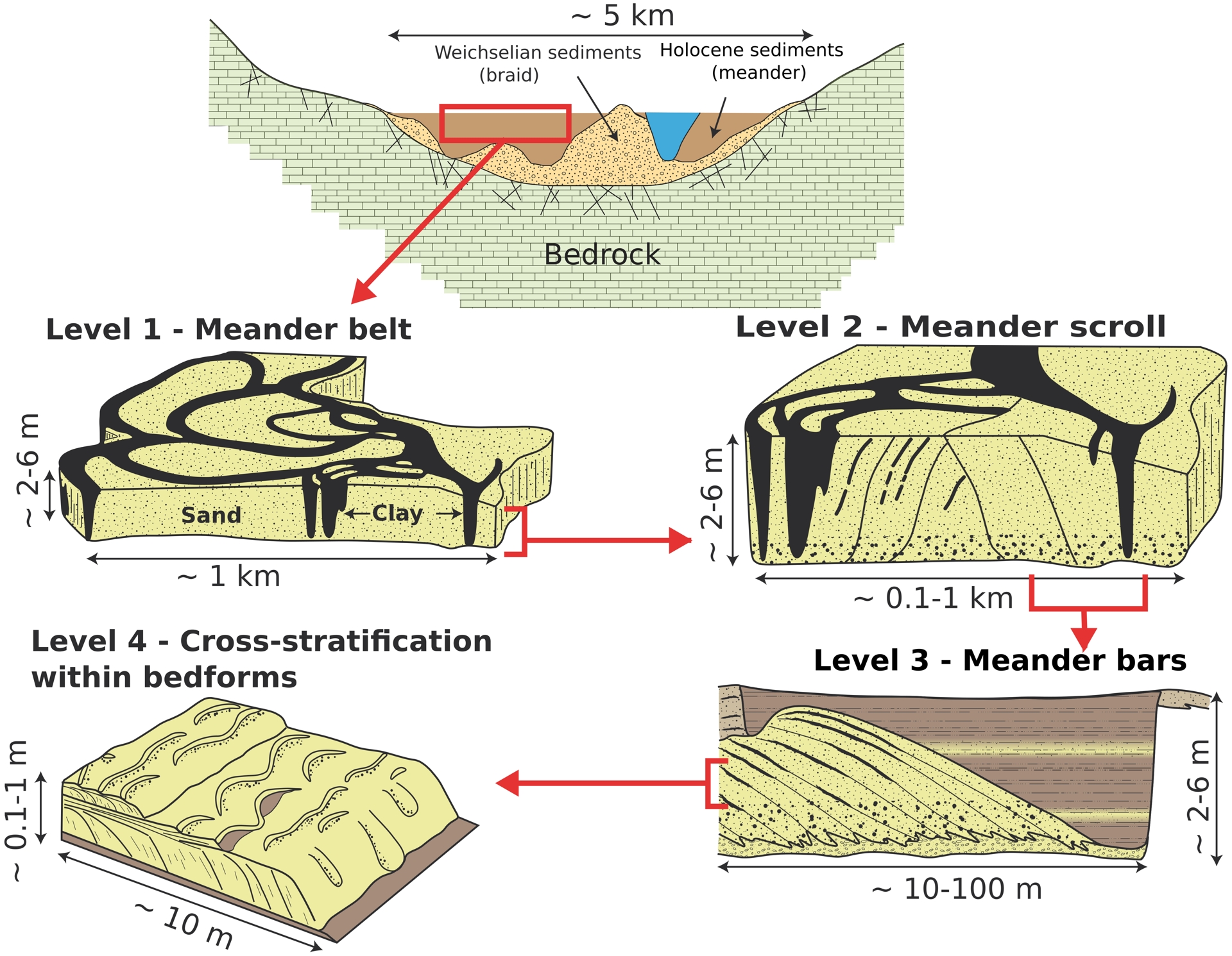
A.2. Field characterisation and numerical modeling of alluvial heterogeneity
The heterogeneities of alluvial aquifers can be assessed directly in the field through outcrops, trenches, or boreholes (Heinz et al., 2003; Hornung and Aigner, 1999; Klingbeil et al., 1999; Bertran et al., 2025; Malenda et al., 2019), or indirectly via geophysical imaging methods. While sedimentological analysis provides detailed lithofacies descriptions along 1D or 2D profiles, the data are localized and challenging to interpolate. Geophysical methods, on the other hand, deliver broader spatial 2D/3D data but often lack resolution for smaller-scale heterogeneities.
Numerical methods offer the possibility to create fully spatialized models of alluvial aquifers (Bayer, Huggenberger, et al., 2011; Comunian et al., 2011), resolving the different scales of sediment heterogeneities, and potentially conditioned by field data (Zappa et al., 2006; Bianchi and C. Zheng, 2016; Sun et al., 2008; Teles et al., 2004; Y. Zhang et al., 2013). Geostatistical methods reproduce the geometric characteristics of an alluvial reservoir, without taking into account the reservoir construction history or the processes behind it. In object-based methods, each sedimentary body is treated as an object, discretized on a grid or continuously modeled by surfaces (Jacquemyn et al., 2019). The domain is filled using probability laws describing both the spatial distribution and the size and orientation of the objects, together with laws of attraction/repulsion between objects. In pixel-based methods, training images are used to define the geostatistical characteristics of sedimentary facies. Realizations are then performed following facies ordering rules (Beucher and D. Renard, 2016; Tahmasebi, 2018). Geostatistical models can be easily conditioned by field data, and low computation times enable a large number of realizations to be generated. On the other hand, results sometimes lack geological realism. Process-based or genetic models aim to reproduce the evolution of a fluvial systems and the associated sediment deposits through a simplification of the physical laws of flow and sediment transport (Camporeale et al., 2007). Because computation times can be very long, deterministic models are generally limited to simulating the morphodynamic evolution of the active channel of a fluvial system on time scales of a few hundred to thousands of years (Van De Lageweg et al., 2016). Finally, mixed stochastic-genetic models (forward model—Lopez, 2003 or reverse—Parquer et al., 2020) use a deterministic approach to compute the channel-form evolution through time, but do only mimic the sedimentary processes with geometrical rules to build the alluvial plain heterogeneity.
A.3. Impact of alluvial plain heterogeneity on ground water fluxes—a synthetic case example
Meandering fluvial systems are characterized by highly sinuous channels (sinuosity > 1.5). The evolution of meander loops in time can lead to neck cutoffs (Gao and Li, 2024) and abandoned oxbow lakes that are filled with fine sediments and organic matter (Jordan and Pryor, 1992). Head gradients along meander loops induce significant SW–GW fluxes across pointbars (Cardenas, 2008; Cardenas, 2009; Boano, Camporeale, Revelli and Ridolfi, 2006; Boano, Camporeale and Revelli, 2010). On the contrary, mud plugs in abandoned meander loops create extensive permeability barriers within the alluvial plain. Here, we use the Flumy genetic sedimentary model Lopez et al. (2008), https://flumy.minesparis.psl.eu/) coupled with hydrogeological model to investigate with synthetic cases the effects of alluvial plain heterogeneity on GW flow and water level in an alluvial aquifer.
Flumy is a model that uses stochastic and process-based approaches to simulate meandering channelized reservoirs. It describes channel evolution through time using physical equations from hydraulic studies (Ikeda et al., 1981), with constant section, slope, and flow. Sedimentary facies are deposited at specific locations in the floodplain, depending on the distance to the channel or a specific process. Sandy point-bar is deposited inside meander loops, while floods produce fine-grained overbank deposits, contributing to channel aggradation. Levee breaches are at the origin of crevasse splays, and channels abandoned after neck cutoff or avulsion are filled with mudplug facies.
Here, Flumy generates a simple 7 km-long, 3 km-wide, 10 m-thick floodplain heterogeneity model. The initial domain is filled with sand facies. The 50 m-wide and 6 m-deep channel is initially straight with small curvature perturbations and flows from west to east. Flumy is run without overbank flood (no vertical accretion) nor avulsion for a certain number of iterations, until the sinuosity is well developed (Dcurve/Dstraight = 2.2), producing meander neck cut-offs and mud plugs. The lateral migration of the channel meanders leads to the deposition of sandy point bars, a facies identical to the initial domain fill. Thus, mud plugs in meanders abandoned after neck cut-off are the only source of heterogeneity in the floodplain. From this heterogeneous model (Figure 2d), a reference homogeneous model is derived by replacing the mud plug facies by sand (Figure 2a).
The hydrofacies values are derived from the literature (Morris and A. I. Johnson, 1967; Urumović and Urumović Sr., 2014). The pointbar sand has a hydraulic conductivity of 2.9 × 10⁻³ m⋅s−1 while the mudplug has a conductivity of 1.6 × 10⁻⁹ m⋅s−1.
The GW flow simulations for both models, homogeneous and heterogeneous, are performed using the 8.1 version of Feflow (Diersch, 2013). The aquifer is supposed to be in a confined state. The simulation domain is subjected to a 0.4‰ regional hydraulic gradient with constant Dirichlet conditions of 9.5 and 7.5 m upstream and downstream. The river’s hydraulic head decreases linearly along the river channel from 9 m to 7 m, representing that it is draining the aquifer. A 30-day flood wave scenario was applied to the riverline BC, with a 3 m increase in the first 15 days and a return to initial state level in the last 15 days.
The resulting simulated head and Darcy flux fields in Figure 2 for the peak flow condition (t = 15 days) are shown for a location between two active meanders (Figure 2d), with the occurrence of a mudplug filled meander.
These results, below the mudplug (Figure 2b, c), and cross-section view (Figure 2e, f), exhibit a doubling of Darcy velocity (from 10 to 20 cm/day) below the mudplug, and a modification of the flow direction. The heterogeneity affects the direction of GW flow beneath the mudplug: the mudplug’s barrier effect tends to reorient the flow in the direction that is orthogonal to the mudplug, pushing downward flow below it. These results, in terms of flow direction and magnitude, confirm that the occurrence of large sedimentary heterogeneity, such as abandoned meander mud plug, can generate a preferential flow path for GW flow. The influence of significant heterogeneity on hydraulic head is restricted to the heterogeneity perimeter, however its effect on flow velocity extend across the full inter-meander area. This means that it could be “easily missed” by a classical data set where only a few piezometers would be available, highlighting the need for geophysical data. This implies that such features could be overlooked in conventional data with sparse piezometer coverage, underscoring the importance of incorporating geophysical data.
The common approach for GW modeling involves calibrating hydrodynamical parameters by comparing simulated with observed hydraulic head, neglecting flow velocity. Consequently, the influence of sedimentary heterogeneity on flow velocity may pose a significant challenge for applications like contamination and heat transport or flow quantification.
Appendix B Physical equations
B.1. GW flow equations
The mass balance equation used to calculate GW (GW) flow is:
| \begin {equation}\label {eq:flow_eq} \nabla \cdot \left (\dfrac {k \bar {k}_r(S_w) \rho _w}{\mu _w} (\nabla p - \rho _w g) \right ) = \dfrac {\partial (\rho _w n S_{w})}{\partial t} + \rho _w q, \end {equation} | (1) |
B.2. Heat transport equations
The heat transport is described by the advection-diffusion equation:
| \begin {equation}\label {eq:heat_transport} \nabla [\lambda \,\nabla T -\rho _{w}\,C_{w}\,q\,T] = \rho \, C\, \dfrac {\partial T}{\partial t}, \end {equation} | (2) |
B.3. Electrical equations
The equations and theoretical models describing electrical current flow in materials are detailed in Telford et al. (1990), particularly for applications in electrical resistivity sounding and tomography. These models combine Ohm’s law with the governing equation for electrical potential, resulting in Laplace’s or Poisson’s equations.
Ohm’s law in a conductive medium is expressed as:
| \begin {equation}\label {eq:ohm} \mathbf {J} = \sigma \mathbf {E}, \end {equation} | (3) |
The electric field relates to the electrical potential 𝜙 by:
| \begin {equation}\label {eq:efield} \mathbf {E} = - \nabla \phi . \end {equation} | (4) |
Combining these and applying the principle of conservation of charge (no accumulation of charge in steady state):
| \begin {equation}\label {eq:charge} \nabla \cdot \mathbf {J} = Q, \end {equation} | (5) |
Substituting Equations (3) and (4) into (5), we get the governing equation for the electrical potential:
| \begin {equation}\label {eq:governing} \nabla \cdot (\sigma \nabla \phi ) = -Q. \end {equation} | (6) |
In regions without current sources, Q = 0, this reduces to Laplace’s equation:
| \begin {equation}\label {eq:laplace} \nabla \cdot (\sigma \nabla \phi ) = 0. \end {equation} | (7) |
B.4. Poro-elastic wave equations
Porous materials are made of a solid phase (called the frame) and of a fluid phase, and can be considered as an interconnected network of pores inside the solid (Pride et al., 2004).
Air and/or water can play the role of the fluid and grains the solid. Poroelastic materials are most of the time modeled using the Biot theory (Biot, 1956a; Biot, 1956b). The differential or “strong” formulation of the poroelastic wave equations can be written as in Carcione (2007) and Carcione (2014).
The related system of equations has seven wave eigenvalues related to seven wave velocity modes (instead of five for the elastic case). Those wave velocities are ± VpFAST, ± VpSLOW, ± Vs and 0. The shear velocity Vs and the fast and slow P-wave velocities (VpFAST and VpSLOW) can be expressed as (Sidler et al., 2013):
| \begin {eqnarray} V_s &=& \sqrt {\dfrac {\mu }{a_1}}, \end {eqnarray} | (8) |
| \begin {eqnarray} V_{p_{\mathrm {FAST}}} &=& \sqrt {\dfrac {-b_1 + \sqrt {\Delta }}{2 a_1}}, \end {eqnarray} | (9) |
| \begin {eqnarray} V_{p_{\mathrm {SLOW}}} &=& \sqrt {\dfrac {-b_1 - \sqrt {\Delta }}{2 a_1}}, \end {eqnarray} | (10) |
| \begin {eqnarray*} a_1 &=& \rho _{11} \rho _{22} - \rho _{12}^2, \\ b_1 &=& -S \rho _{22} - R \rho _{11} + 2 ga \rho _{11}, \\ c_1 &=& S R - ga^2, \\ \rho _{11} &=& \rho + \rho _f n (a - 2), \\ \rho _{12} &=& n \rho _f (1-a), \\ \rho _{22} &=& a \rho _f n, \\ S &=& \lambda + 2 \mu , \\ R &=& M n^2, \\ \Delta &=& b_1^2 - 4 a_1 c_1, \\ ga &=& M n (\alpha - n). \end {eqnarray*} |
The different parameters of the poroelastic model are: n (porosity), 𝜌 (density of the satured medium), 𝜌s (density of the solid), 𝜌f (density of the fluid), 𝜌w (apparent density), Ks (incompressibility modulus of the solid matrix), Kf (incompressibility modulus of the fluid), Kfr (incompressibility modulus of the porous frame), 𝜅 (permeability of the solid matrix), 𝜂 (fluid viscosity), a (tortuosity), 𝜆 (Lamé coefficient of the saturated matrix), 𝜆s (Lamé coefficient in the solid matrix), 𝜇 (shear modulus). Some of these parameters are a combination of the others.
Biot’s characteristic frequency fc defines the transition between two poroelastic regimes (with or without attenuation) and is given as follows (see Biot (1956b), Carcione (2007) and Morency and Tromp (2008)):
| \begin {equation}\label {fc_regime} f_c = \min \left (\dfrac {\eta n}{2 \uppi a \rho _f \kappa }\right ). \end {equation} | (11) |
The maximum frequency range fmax of the source is such that fmax < fc. Therefore, in the experimental and numerical modeling of unconsolidated granular media under study, we choose to stay in the poroelastic regime without attenuation.