


 CC-BY 4.0
1. Introduction
The absolute entropy of the moist-air atmosphere was first defined by Hauf and Höller (1987) but was never calculated or studied for its own sake until recently1 . Similarly, the absolute entropy of sea-salt oceans has already been defined in the papers by Millero and Leung (1976, hereafter ML76) and Millero (1983, hereafter M83), recalled in Sharqawy et al. (2010) and Qasem et al. (2023) but not in Nayar et al. (2016), without any attempt until now to calculate it from in-situ measurements or from numerical model outputs.
These “absolute” definitions of the entropies of the atmosphere and the ocean are obtained from the reference values of entropies available in all thermodynamic and thermochemical tables2 , this for the various species N2, O2, Ar, CO2 and H2O making up the moist-air atmosphere, and for liquid water, Na+, Mg2+, …, Cl−, $\mathrm{SO}_4^{2-}, \ldots $ for the seasalt ocean.
These absolute reference values have been computed by applying the third law of thermodynamics, which, following the works of Nernst (1906) and then Planck (1911; 1917), stipulates that the entropies of the most stable crystalline state of all bodies cancel out at the absolute zero of temperature. This third law is used for the calorimetric calculations $S(T)=S(0)+\int _0^T c_p(T')\, \mathrm{d}\ln (T')+\sum _k L_k(T_k)/T_k$ based on S(T = 0 K) = 0, with the integral of the specific heat capacities cp(T) and including the impact of all phase changes at temperatures Tk with the latent heats Lk(Tk). The third law also corresponds to the statistical calculations S(T) = 0 + k ln(W), where the 0 term indicates that no other arbitrary term must be added, where k is the Planck–Boltzmann constant, and where W, the number of quantum configurations, must be evaluated at the absolute temperature T for all translational (Sackur–Tetrode–Planck), rotational, and vibrational degrees of freedom of atoms and molecules. Note that if the original third law corresponds to both S(T = 0 K) = 0 in the calorimetric formula and to the 0 term in the statistical one, this original definition of Planck (1911; 1917) must be nowadays amended by considering possible residual entropies S(0)≠0 at 0 K in the calorimetric formula only (but not the statistical one) and for a few species like H2O (ice Ih), due to the next computations of Pauling (1935) and Nagle (1966).
Differently, almost all other definitions of the quantities called “entropies” in atmospheric and oceanic studies deviate from these methods by choosing other reference values that differ from both the calorimetric and statistical-quantum values provided by the third law of thermodynamics. More precisely, the alternative definitions are obtained by arbitrarily cancelling out these reference entropy values at the zero Celsius temperature or the triple point at 0.01 °C (instead of zero Kelvin) for dry air, liquid water, and sea salts3 . The fact that the values of the reference entropies have no impact in most oceanographic applications, unless one wants to calculate and study the entropy of seawater itself, is a key reason for the dominant approach where these reference entropies are defined arbitrarily, as in TEOS10.
It is within this framework that the TEOS104 software (McDougall, Feistel, et al., 2010) has been designed, with thermodynamic functions computed with greater consistency from the Gibbs function fitted on more numerous and more recent observed datasets than before. However, although Millero (2010, p. 19) explained that “(…) new TEOS-10 (…) will be very useful to modelers examining the entropy and enthalpy of seawater,” this TEOS10’s values can be amended to correspond to the third law of thermodynamics and Millero’s previous papers concerning the calculation of seawater entropy, due to arbitrary redefinitions made in TEOS10 of the reference entropies of liquid water and ocean salts. Moreover, there have been a few papers, other than those already cited, where the absolute definitions of entropies have been explicitly mentioned or even taken into account: Lemmon et al. (2000) for the dry air; Feistel and Wagner (2005; 2006) for the liquid water.
Consequently, the aim of the present paper is to compute and study the absolute seawater entropy state variable on concrete cases (observed vertical profiles and surface analyzed datasets, as shown in the next Part II). The chosen methodology described in Part I consists of reconciling the TEOS10 formulation, with all its advantages, with the use of absolute values of reference entropies, as prescribed by Millero and available in all thermodynamic tables.
The paper is organized as follows. I explain in Section 2 the way the standard seawater entropy is presently computed in the reference TEOS10 software (see Section 2.1). I then explained in the Section 2.2 why there is a need to update the computations of this standard seawater entropy, by taking into account the absolute value for the (pure) liquid-water entropy recalled in the Section 2.3, and also the absolute for the sea-salts entropies, first computed at 25 °C in the Section 2.4, and then at 0 °C in the Section 2.5, before to show in the Section 2.6 how it is possible to modify the TEOS10 relationships to compute the seawater entropy for all conditions of temperature, salinity and pressure.
Several comparisons with observations and analysed surface datasets are conducted in the second part of the paper (Marquet, 2026). In this first theoretical part are shown in Section 3 two numerical applications. The impact of the salinity is studied in Section 3.1 with a comparison between the old Millero and other papers, including the standard TEOS10 and the new absolute seawater entropy formulations. I show that several problems unfortunately prevent the use of the “relative” entropy formulation considered by Millero in 1976 and 1983. Moreover, this “relative” entropy formulation did not really take into account the absolute values of entropies and has never been used since then. This therefore justifies basing the present approach on the more modern formulation of TEOS10, with the sole addition of taking into account the absolute values of the reference entropies for liquid water and ocean salts. The classic t − SA oceanic diagrams are plotted in Section 3.2 by adding the new absolute isentropic (iso-entropy) lines to the isopycnic (iso-density) lines. Furthermore, I describe in Section 3.3 other more general situations in physics where the absolute values of entropies impact different phenomena, with detailed computations shown in the Supplementary Materials (Marquet, 2025, hereafter referred to as “SM”), as well as answers to FAQs regarding the interest, or not, of studying the absolute entropies of the atmosphere and oceans.
I finally recall in the concluding Section 4 the main results of the paper.
2. Computations of seawater entropy
2.1. The standard TEOS10 present version
The aim of this section is to recall how the seawater entropy is calculated in the current standard version of TEOS10, and to show where the reference entropy values for liquid water and sea salts appear.
The specific entropy5 𝜂 called “entropy of seawater” is computed in McDougall, Feistel, et al. (2010, Eq. (2.10.1), p. 20)6 as a derivative of the specific seawater Gibbs’ function g:
| \begin {equation}\label {eq_TEOS10_eta_dg_dt} \eta (S_{\mathrm {A}}, t, p)=\left .{-}\frac {\partial g}{\partial t}\right |_{S_{\mathrm {A}},p} = \left .{-}\frac {1}{40} \frac {\partial g}{\partial y}\right |_{S_{\mathrm {A}},p}, \end {equation} | (1) |
The specific free enthalpy g = G/m (with m = 1 kg) of a multi-component dilute aqueous electrolyte solution was previously derived according to Feistel and Hagen (1995, Eq. (4.9), p. 266) from the practical osmotic factor considered in Lewis and Randall (1961, Eq. (23-4), p. 334; hereafter LR61) and Falkenhagen and Ebeling (1971, Eq. (116), p. 40), leading to a formulation that can be rewritten as
| \begin {eqnarray} g = (1-C) \times \mu ^0_{w}(T,P)+ C\times \mu ^0_{s}(T,P) + \sum _a \frac {X_a}{M_{s}} R\,T\,C\, \ln \left [X_a\frac {C}{1-C} \frac {M_{w}}{M_{s}}\right ] - \frac {\left [\sum _a N_a Z_a^2 e^2/D(T,P)\right ]^{3/2}} {\sqrt {36\uppi \nu (T,P)kTN_{w}}}, \label {eq_FH95_4_9} \end {eqnarray} | (2) |
According to McDougall, Feistel, et al. (2010, Eq. (2.6.1), p. 15) the TEOS10 Gibbs function (2) is split in two and written as the sum of the “pure water” (W) and “salinity” (S) parts
| \begin {equation}\label {eq_TEOS10_g_x_y_z} g(x,y,z) = g^{W}_{\mathrm {Fei03}}(y,z) + g^{S}_{\mathrm {Fei08}}(x,y,z), \end {equation} | (3) |
| \begin {equation}\label {eq_TEOS10_eta_x_y_z} \eta (x,y,z) = \eta ^{W}_{\mathrm {Fei03}}(y,z)+ \eta ^{S}_{\mathrm {Fei08}}(x,y,z), \end {equation} | (4) |
The two Gibbs functions $g^{W}_{\mathrm{Fei03}}(y,z)$ and $g^{S}_{\mathrm{Fei08}}(x,y,z)$ were previously computed by Feistel (2003, Table 10-27, p. 93) and Feistel (2008, Table 17, p. 1666), respectively, as series expansions of xi yj zk:
| \begin {equation} g^{W}_{\mathrm {Fei03}}(y,z) = \sum _{j=0}^{7} \sum _{k=0}^{6} g_{0jk}\, y^jz^k \label {eq_TEOS10_Gw_y_z} \end {equation} | (5) |
| \begin {equation} g^{S}_{\mathrm {Fei08}}(x,y,z) = \!\sum _{j=0}^{6} \sum _{k=0}^{5} \left [g_{1jk} x^2\ln (x)+ \sum _{i=2}^{6} g_{ijk} x^i\right ]\! y^jz^k, \label {eq_TEOS10_Gs_y_z} \end {equation} | (6) |
According to (1) applied to (3), and thus to (5) and (6), the entropy coefficients corresponding to (4) are 𝜂ijk = −(j + 1)gi,j+1,k/40 and correspond to the relationships shown in Tables 1 and 2, which enable us to compute directly the TEOS10 seawater entropy without using the TEOS10 software7 .
The “pure-liquid-water” part of the seawater entropy function as computed from the TEOS10 software (see the gijk coefficients in Appendix G, p. 155), where y = t/(40 °C) and z = p/(100 MPa) are two dimensionless variables
| ${\begin{array}{@{}r@{~ }c@{~ }l@{}} \overbrace{\eta ^{W}_{\mathrm{Fei03}}(y,z)}^{\text {``pure-Water''}} &=& \overbrace{\{\eta _{w0}\}}^{\text {``???''}} + \left (\dfrac {1} {40}\right ) \overbrace{({-}5.90578347909402)}^{(-g_{010})} + \left (\dfrac {1}{40}\right ) \left [270.983805184062z\right .\\ && -\; 776.153611613101z^2 + 196.51255088122 z^3 - 28.9796526294175 z^4\\ && +\; 2.13290083518327 z^5 +24715.571866078 y -2910.0729080936yz\\ && +\; 1513.116771538718 yz^2 -546.959324647056 y z^3 + 111.1208127634436 y z^4\\ && -\; 8.68841343834394 y z^5 - 2210.2236124548363 y^2 + 2017.52334943521 y^2 z\\ && -\; 1498.081172457456 y^2 z^2 + 718.6359919632359 y^2 z^3 -146.4037555781616 y^2 z^4\\ && +\; 4.9892131862671505 y^2 z^5 +592.743745734632 y^3 - 1591.873781627888 y^3 z\\ && +\; 1207.261522487504 y^3 z^2 -608.785486935364 y^3 z^3+ 105.4993508931208 y^3 z^4\\ && -\; 290.12956292128547 y^4+973.091553087975 y^4 z - 602.603274510125 y^4 z^2\\ && +\; 276.361526170076 y^4 z^3-32.40953340386105 y^4 z^4+ 113.90630790850321 y^5\\ && -\; 21.35571525415769 y^6 +67.41756835751434 y^6 z- 381.06836198507096 y^5 z\\ && +\; 133.7383902842754 y^5 z^2-49.023632509086724 y^5 z^3\left .\! \right ]. \end{array}}$ |
The “saline” (sea-salts) part of the seawater entropy function as computed from the TEOS10 software (see the gijk coefficients in Appendix H, p. 156), with the dimensionless concentrations C = XA = SA/1000 and XSO = SSO/1000 and the dimensionless variables x2 = SA/(40.188617 g⋅kg−1), y = t/(40 °C) and z = p/(100 MPa), where SA is the absolute salinity in units of g⋅kg−1 and SSO = 35.16504 g⋅kg−1 is a standard seawater salinity (see Table D.4, p. 145)
| ${\begin{array}{@{}r@{~ }c@{~ }l@{}} \overbrace{\eta ^{S}_{\mathrm{Fei08}}(x,y,z)}^{\text {``Salinity''}} &=& \overbrace{\{\eta _{s0} - \eta _{w0}\}}^{\mbox{``???''}} \times \left (\dfrac {S_{\mathrm{A}} - S_{\mathrm{SO}}}{1000}\right ) + \left (\dfrac {1} {40}\right )\left [\! \right . \overbrace{({-}168.072408311545)}^{({-}g_{210})}x^{2}\\ && -\; 851.226734946706 \ln (x) x^2 -729.116529735046 x^2 z+ 343.956902961561 x^2 z^2\\ && -\; 124.687671116248 x^2 z^3 +31.656964386073 x^2 z^4 - 7.04658803315449 x^2 z^5\\ && +\; 493.407510141682 x^3 -543.835333000098 x^4 + 196.028306689776 x^5\\ && -\; 36.7571622995805 x^6 +137.1145018408982 x^4 y -148.10030845687618 x^4 y^2\\ && +\; 68.5590309679152 x^4 y^3 -12.4848504784754 x^4 y^4 +22.6683558512829 x^4 z\\ && +\; 175.292041186547 x^3 z-83.1923927801819 x^3 z^2 +29.483064349429 x^3 z^3\\ && +\; 86.1329351956084 x^3 y -766.116132004952 x^3 y z +108.30162043765552 x^2 y^4\\ && -\; 51.2796974779828 x^3 y z^3 +30.068211258562 x^3 y^2 +1380.9597954037708 x^3 y^2 z\\ && -\; 3.50240264723578 x^3 y^3 -938.26075044542 x^3 y^3 z -1760.062705994408 x^2 y\\ && +\; 675.802947790203 x^2 y^2 -365.7041791005036 x^2 y^3 +108.3834525034224 x^3 y z^2\\ && -\; 12.78101825083098 x^2 y^5 +1190.914967948748 x^2 y^3 z\\ && -\; 298.904564555024 x^2 y^3 z^2+145.9491676006352 x^2 y^3 z^3\\ && -\; 2082.7344423998043 x^2 y^2 z +614.668925894709 x^2 y^2 z^2\\ && -\; 340.685093521782 x^2 y^2 z^3 +33.3848202979239 x^2 y^2 z^4\\ && +\; 1721.528607567954 x^2 y z -674.819060538734 x^2 y z^2+ 356.629112415276 x^2 y z^3\\ && -\; 88.4080716616 x^2 y z^4+15.84003094423364 x^2 y z^5\left .\! \right ]. \end{array}}$ |
The way in which the two parts of g are defined in (3) can be understood by rewriting the first line of (2) using the definition $\mu ^0_{w} = h_{w}-T\, \eta _{w}$ and $\mu ^0_{s} = h_{s}-T\, \eta _{s}$ for the pure-liquid water and sea-salts chemical potentials, with the concentration C = SA/1000 in kg⋅kg−1 depending on the absolute salinity SA in g⋅kg−1. Therefore, the first-order constant terms 𝜂w0 and 𝜂s0 (independent of T and P) of the entropy 𝜂 impact the Gibbs function via the terms (1 − SA/1000) 𝜂w0 + (SA/1000) 𝜂s0, which can be rewritten as [𝜂w0] + [(𝜂s0 −𝜂w0)(SA/1000)]. This explains the natural splitting of this sum in the two TEOS10’s Tables 1 and 2 (for $\eta ^{W}_{\mathrm{Fei03}}$ and $\eta ^{S}_{\mathrm{Fei08}}$) into the two bracketed “pure-water” [𝜂w0] and “salinity” [(𝜂s0 −𝜂w0)(SA/1000)] parts, respectively. Other linear and non-linear variables terms generated by the three lines of (2) are similarly cast into the “pure-water” and “salinity” parts of g, and thus of 𝜂. In particular, the second line of (2) explains the term x2 ln(x) with x2 = SA/40.188617 = 24.88267C.
Therefore, the reference values of the entropies do not impact the pure-water part of the seawater entropy, since [𝜂w0] is a mere constant with no physical meaning (null differential). Differently, the linear first-order salinity term must have a physical impact on the computation of the seawater entropy. Indeed, its differential (𝜂s0 −𝜂w0)(dSA/1000) is a priori different from zero and depends on the difference of the two reference values. Thus, it depends on both 𝜂s0 and 𝜂w0, which must be determined in order to compute the absolute value of the seawater entropy 𝜂 in (4) from Tables 1 and 2.
The first choice retained in pre-TEOS10 formulations was to arbitrarily set 𝜂w0 = 0 in order to cancel the pure-water entropy at the triple-point conditions: $\eta ^{W}_{\mathrm{Fei03}}(T_{t},p_{t})=0$ (ibid., Eq. (G.2), p. 155). In fact, in the present version of TEOS10 software, the term 𝜂w0 is set to − g010/40 ≈−5.9056/40 ≈ 0.14764 instead, and (𝜂s0 −𝜂w0) is set to − g210/40 ≈−168.0724/40 ≈ 4.2018 in order to arrive at the cancellation of the whole seawater entropy 𝜂(SSO,tSO,pSO) for the arbitrary standard conditions SSO = 35.16504 g⋅kg−1, tSO = 0 °C, and pSO = 0 dbar (see the explanations p. 155 and Eq. (2.6.6), p. 17 of ibid.).
2.2. A need to update the seawater entropy
The seawater entropy can be written as 𝜂(x,y,z) =𝜂 w0 + (𝜂s0 −𝜂w0)(SA/1000) + (⋯ ), where (⋯ ) represents the non-linear higher-order terms in x2, y or z. Therefore, the first-order terms of the vertical gradient ∂𝜂/∂z and the turbulent flux $\overline{w'\eta '}$ are the product of the measurable quantities ∂SA/∂z and $\overline{w' S'_{\mathrm{A}}}$ by the difference in reference entropy (𝜂s0 −𝜂w0). Then, since the entropy is a thermodynamic state function, the difference of 𝜂 between two points, and thus its gradients and turbulent fluxes, cannot be arbitrary and cannot be either positive, null, or negative, depending on the values and signs of 𝜂s0 −𝜂w0. This means that it is not possible to modify or arbitrarily set 𝜂s0 and/or 𝜂w0 to this or that value unless modifying the entropy budget (d𝜂/dt = ⋯ ), and thus the second law of thermodynamics.
It may be decided not to bother with entropy calculations, since the reference entropy values have no impact on the other thermodynamic variables (specific volumes, heat capacities, expansion coefficients, sound speeds, osmotic pressure, etc.) and only impact the entropy, Helmholtz free energy, and Gibbs free enthalpy functions. But in this case, we have to go right to the end of the consequences and refrain from calculating values of these three functions, leaving these three quantities undetermined to within a function of salinity.
Differently, one of the aims of TEOS10, as Millero reminded us, is to provide precise values for these three functions. So there is no choice if you want to calculate these three functions: you have to leave no room for arbitrariness and trust the recommendations of general thermodynamics. Here lies the strong motivation for using non-arbitrary values for not only the difference in reference entropies 𝜂s0 −𝜂w0, but in fact for both 𝜂s0 and 𝜂w0, and thus to use the absolute, third-law values of them defined in thermodynamics.
In addition, although the formulations of ML76 and M83 brought a clear theoretical improvement in taking into account the absolute reference entropies of liquid water and sea salts, the analytical and numerical formulation seems somewhat anomalous (see Section 3.1). As a consequence, Millero’s calculations had to be restated using more recent data and methods.
2.3. The absolute entropy of pure liquid water
I recall in the second line of Table 3 that the value of the absolute entropy of (pure) liquid water is well-known since at least LR61 (Table 12.3, p. 137), who published values corresponding to
| \begin {eqnarray} \eta _{w0/\mathrm {LR61}}(25~\mbox {{\textdegree }C}) &\approx & 16.73 \times 4.184 \approx 70.00~\mathrm {J}{\cdot }\mathrm {K}^{-1}{\cdot } \mathrm {mol}^{-1}, \label {Eq_ML76_M83_eta_w0_mol}\end {eqnarray} | (7) |
| \begin {eqnarray} \eta _{w0/\mathrm {LR61}}(25~\mbox {{\textdegree }C}) &\approx & \frac {70.00} {0.018015} \approx 3885.65~\mathrm {J}{\cdot }\mathrm {K}^{-1}{\cdot } \mathrm {kg}^{-1}. \label {Eq_ML76_M83_eta_w0_kg} \end {eqnarray} | (8) |
The molar mass (M, in g⋅mol−1), mole fraction (X, in mol⋅mol−1) and absolute entropies (S, in J⋅K−1⋅mol−1, “relative” to S(H+) = 0), computed at 25 °C and 0.1 MPa, for the pure liquid water (H2O)liq. and the main seasalts (cations and anions). Values of M(M82) are from Millero (1982, Table IV, p. 428); those of X(M83) are from M83 (Table X, p. 35) with about half the values of X(M83) normalized to a sum of 1; those of M(TEOS10) and X(TEOS10) are from McDougall, Feistel, et al. (2010, Table D.3, p. 137), with the molar fractions obtained from the rounded values of Millero, Feistel, et al. (2008, Table 3, p. 60). The absolute entropies “M83” (from Table X, p. 35) are the same as those in ML76 (Table 32, p. 1071) and are in fact those previously listed in “LR61” (Table 25.7, p. 400-401). The more recent entropies “G92” are from Grenthe, Fuger, et al. (1992, “NEA-TDB” for “Nuclear Energy Agency and Thermodynamic Data Bank”, see the “Selected auxiliary data” p. 64–83), which are still retained in Grenthe, Gaona, et al. (2020). The numbers in parentheses refer to the uncertainty in the corresponding last digits, with, for instance, 96.0626(50) meaning 96.0626 ± 0.0050.
| M(M82) | X(M83) | S(LR61/M83) | M(TEOS10) | X(TEOS10) | S(G92) | |
|---|---|---|---|---|---|---|
| (H2O)liq. | 70.00 | 18.015268 | 69.95(3) | |||
| (H+) | (0.0) | (0.0) | ||||
| Na+ | 22.9898 | 0.4182121 | 60.2 | 22.98976928(2) | 0.4188071 | 58.45(15) |
| Mg2+ | 24.305 | 0.0475583 | −118 | 24.3050(6) | 0.0471678 | −137(4) |
| Ca2+ | 40.08 | 0.0091726 | −55.2 | 40.078(4) | 0.0091823 | −56.2(10) |
| K+ | 39.102 | 0.0091126 | 102.5 | 39.0983(1) | 0.0091159 | 101.2(2) |
| Sr2+ | 87.62 | 0.0000800 | −39.3 | 87.62(1) | 0.0000810 | −31.5(20) |
| Cl− | 35.453 | 0.4875415 | 55.2 | 35.453(2) | 0.4874839 | 56.6(2) |
| $\mathrm{SO}_4^{2-}$ | 96.0576 | 0.0252171 | 17.2 | 96.0626(50) | 0.0252152 | 18.5(4) |
| $\mathrm{HCO}_3^{-}$ | 61.0172 | 0.0017255 | 95.0 | 61.01684(96) | 0.0015340 | 98.4(5) |
| Br− | 79.904 | 0.0007552 | 80.8 | 79.904(1) | 0.0007520 | 82.55(20) |
| $\mathrm{CO}_3^{2-}$ | 60.0092 | 0.0002000 | −51.3 | 60.0089(10) | 0.0002134 | −50(1) |
| $\mathrm{B(OH)}_4^{-}$ | 78.8396 | 0.0000750 | ( ≈100) | 78.8404(70) | 0.0000900 | (102.5) |
| F− | 18.9984 | 0.0000500 | −9.6 | 18.9984032(5) | 0.0000610 | −13.8(8) |
| OH− | (−) | (−) | −10.5 | 17.00733(7) | 0.0000071 | −10.9(2) |
| $\mathrm{B(OH)}^{\mathrm{aq.}}_{3}$ | 61.8322 | 0.0003001 | ( ≈50) | 61.8330(70) | 0.0002807 | 162.4(6) |
| $\mathrm{CO}^{\mathrm{aq.}}_{2}$ | (−) | (−) | (−) | 44.0095(9) | 0.0000086 | 119.36(60) |
| Mean | 31.405 | 1.0000000 | 47.52 | 31.404(1) | 1.0000000 | 46.74(40) |
I will retain for this study the smaller value
| \begin {equation} \label {eq_eta_w0_NEA_TDB_1992} \eta _{w0}(0~\mbox {{\textdegree }C}) \approx 3513.4 \pm 1.7~\mathrm {J}{\cdot }\mathrm {K}^{-1}{\cdot }\mathrm {kg}^{-1} \end {equation} | (9) |
2.4. The absolute entropy of sea-salts at 25 °C
The mean absolute entropy for sea-salt aqueous ions has already been computed by ML76 (Table 32, p. 1071) and M83 (Table X, p. 35) from the individual values S(LR61/M83) previously published by LR61 (Table 25.7, p. 400–401) and recalled in Table 3. The resulting value was
| \begin {eqnarray} \eta _{s0/\mathrm {M83}}(25~\mbox {{\textdegree }C}) &\approx & \frac {95.01}{1.99944} \approx 47.52~\mathrm {J}{\cdot } \mathrm {K}^{-1}{\cdot }\mathrm {mol}^{-1}, \label {Eq_ML76_M83_eta_s0_mol}\end {eqnarray} | (10) |
| \begin {eqnarray} \eta _{s0/\mathrm {M83}}(25~\mbox {{\textdegree }C}) &\approx & \frac {95.01} {0.062793} \approx 1513.1~\mathrm {J}{\cdot }\mathrm {K}^{-1}{\cdot } \mathrm {kg}^{-1}. \label {Eq_ML76_M83_eta_s0_kg} \end {eqnarray} | (11) |
Therefore, the mean sea-salt molar mass previously derived by ML76 (M2 in Eq. (10) in the Appendix, p. 1074) roughly corresponds to ⟨A⟩ = 62.793/1.99944 ≈ 31.405 g⋅mol−1. More precisely, more relevant definitions were suggested by Millero (1982, Eq. (88), p. 427 and Table IV, p. 428), with the total mole written as nT = nB + (1/2)∑ini and leading to a sum NB + (1/2)∑iNi = 1.0000005 very close to 1 and to MT = NBMB + (1/2)∑iNiMi ≈ 31.3677 g⋅mol−1 indeed indicating double values for all the ions Ni≠NB (i.e., except the non-ionic Boric term). However, these more relevant 1982 definitions were not considered in ML76 and will not be retained in M83.
Note that the sea-salt aqueous ions listed in Table 3 are relative to $\overline{S}^{\circ }_{\mathrm{H}^+}=0$, with, however, no impact of a non-zero value for $\overline{S}^{\circ }_{\mathrm{H}^+}$ on the mean value for the sea-salt entropy. Indeed, a non-zero value ΔS0 for $\overline{S}^{\circ }_{\mathrm{H}^+}$ would lead to a change in the average sea salt entropy corresponding to the weighted sum ∑j(ZjΔS0)Xj = (∑jZjXj)ΔS0, which depends on the valence (ionic charges) Zj and the mole fractions Xj. Fortunately, this sum is zero in the Millero (ML76 and M83) and TEOS10 set-ups thanks to the neutrality property ∑iZjXj = 0 (see the column for Zj × Xj in Table D.3 of McDougall, Feistel, et al., 2010, p. 144).
Moreover, Millero’s articles suffer from the fact that they do not take into account the two species OH− and $\mathrm{CO}^{\mathrm{aq.}}_{2}$ considered in the more recent studies and TEOS10.
Due to all these inaccuracies and outdated references in the papers by ML76 and M83, it was desirable to use updated and more recent values for the sea-salts entropies and concentrations, like the TEOS10’s sea-salts values listed in McDougall, Feistel, et al. (ibid.), Table D.3, p. 144. It was also necessary to use updated values for the molar absolute sea-salt entropies $\Delta _r S^{\circ }_m$, like those listed in the “Selected auxiliary data” in the NEA-TDB Tables IV.1 and IV.2 of Grenthe, Fuger, et al. (1992, S(G92), p. 64–83) and retained in Grenthe, Gaona, et al. (2020), including uncertainty intervals.
The corresponding updated mean values for M(TEOS10) and S(G92) shown in Table 3 are
| \begin {eqnarray} M_{s} \approx 31.404 \pm 0.001~\mathrm {g}{\cdot }\mathrm {mol}^{-1}, \label {Eq_Ms}\end {eqnarray} | (12) |
| \begin {eqnarray} \eta _{s0}(25~\mbox {{\textdegree }C}) \approx 46.74 \pm 0.40~\mathrm {J}{\cdot }\mathrm {K}^{-1}{\cdot }\mathrm {mol}^{-1}, \quad \eta _{s0}(25~\mbox {{\textdegree }C}) \approx 1488.3 \pm 13~\mathrm {J}{\cdot }\mathrm {K}^{-1}{\cdot }\mathrm {kg}^{-1}, \label {Eq_eta_s_25C_kg} \end {eqnarray} | (13) |
2.5. The absolute entropy of sea salts at 0 °C
In order to compute the mean reference sea-salt entropy at 0 °C by using the relationship $S(273.15)=S(295.15)+\overline{C}^{\circ }_{p} \ln (273.15/298.15)$, it is needed to know the mean specific heats of sea salts at constant pressure $\overline{C}^{\circ }_{p}$, for instance by averaging the individual values for each sea salt recalled in Table 4 from several datasets, where individual values are not available for all species. For this reason, three kinds of averaging are made: first with the two main species 0.5% of Na+ and 0.5% of Cl− and the concentrations X(2); then for the four main species Na+, Mg2+, Cl−, and $\mathrm{SO}_4^{2-}$ (for LR61, HH96 and M12) and the concentrations X(4); and then for the whole set of the eight species (for HH96 and M12 only) and the concentrations X(8).
Values of the molar specific heat at constant pressure $\overline{C}^{\circ }_p$ at 25 °C (in J⋅K−1⋅mol−1) for several of the major sea-salt cations and anions, and based on $\overline{C}^{\circ }_p (\mathrm{H}^{+}) = 0$: “LR61” (Table 25-7, p. 400–401) Lewis and Randall (1961, Table 25-7, p. 400–401); “NBS82” from Wagman et al. (1982, Tables p. 2‐47, 2‐50, 2‐57, 2‐83, 2‐260, 2‐267, 2‐299, 2‐328); “CM96” from Criss and Millero (1996, Table 2, p. 1290); “HH96” from Hepler and Hovey (1996, Table 5, p. 647). Conversions from the old unit (cal K−1⋅mol−1) of “LR61” are made with 1 cal = 4.184 J. The values “M12” from Marcus (2012, Table 1.2, p. 12) were with $\overline{C}^{\circ }_p (\mathrm{H}^{+}) = -71~ \mathrm{J}{\cdot }\mathrm{K}^{-1}{\cdot }\mathrm{mol}^{-1}$ and have been transformed for the reference $\overline{C}^{\circ }_p (\mathrm{H}^{+}) = 0$ by taking into account the valences of ions Z (−2, −1, +1, +2). The molar concentrations X (in mol⋅mol−1) are adapted from McDougall, Feistel, et al. (2010, Table D.3, p. 137) recalled in the previous Table 3. The rescaled values lead to a sum of 1 for either the case X(2) where only two major species (Na+ and Cl−) are available, or the case X(4) where four major species (Na+, Mg2+, Cl− and $\mathrm{SO}_4^{2-}$) are available, or the case X(8) where all eight species are available.
| $\overline{C}^{\circ }_p$ | Na+ | Mg2+ | Ca2+ | K+ | Cl− | $\mathrm{SO}_4^{2-}$ | $\mathrm{HCO}_3^{-}$ | Br− | Mean |
|---|---|---|---|---|---|---|---|---|---|
| X(2) | 0.500 | 0.500 | 1.000 | ||||||
| LR61 | 33.1 | (+16.7) | (−37.7) | (9.6) | −126 | (−276) | (⋯ ) | (−130) | −46.5 |
| NBS82 | 46.4 | (⋯ ) | (⋯ ) | (21.8) | −136.4 | (−293) | (⋯ ) | (−141.8) | −45.0 |
| CM96 | 43.01 | (⋯ ) | (⋯ ) | (12.47) | −126.32 | (⋯ ) | (−53.33) | (−131.27) | −41.7 |
| HH96 | 42 | (−16) | (−27) | (12) | −126 | (−276) | (−52) | (−132) | −42.0 |
| M12 | 43 | (−16) | (−27) | (13) | −127 | (−280) | (−53) | (−131) | −42.0 |
| X(4) | 0.42793 | 0.04820 | 0.49810 | 0.02577 | 1.000 | ||||
| LR61 | 33.1 | +16.7 | (−37.7) | (9.6) | −126 | −276 | (⋯ ) | (−130) | −54.9 |
| HH96 | 42 | −16 | (−27) | (12) | −126 | −276 | (−52) | (−132) | −52.7 |
| M12 | 43 | −16 | (−27) | (13) | −127 | −280 | (−53) | (−131) | −52.8 |
| X(8) | 0.41912 | 0.04720 | 0.00919 | 0.00913 | 0.48784 | 0.02524 | 0.00153 | 0.00075 | 1.000 |
| HH96 | 42 | −16 | −27 | 12 | −126 | −276 | −52 | −132 | −51.9 |
| M12 | 43 | −16 | −27 | 13 | −127 | −280 | −53 | −131 | −52.1 |
When available, the order of magnitude and the signs of $\overline{C}^{\circ }_p$ are similar for the 6 species Na+, K+, Cl−, $\mathrm{SO}_4^{2-}$, $\mathrm{HCO}_3^{-}$ and Br−. The discrepancies are larger for Ca2+ and Mg2+, with even not the same signs for Mg2+. However, the value for Mg2+ computed in a recent paper by Caro et al. (2020, Table 7, p. H) is negative (−155) and close to the value −16 − 2 × 71 = −158 published in both HH96 and M12. For this reason the old positive values of LR61 for Mg2+ might be inaccurate.
The mean values computed with 0.5% of Na+ and 0.5% of Cl− are close to −42 to −46 units. The mean values computed with the 4 major species Na+, Mg2+, Cl− and $\mathrm{SO}_4^{2-}$ are more negative (by about 10 units) and remain close to each other (about −53 ± 2 units), which is close to the mean values computed with the more complete set of 8 species (about −52 ± 1 units).
Therefore, the mean specific heat at constant pressure for sea salts may be set to
| \begin {equation}\label {eq_Cp_seasalt_molar} \overline {C}_{p{s}} \approx -52 \pm 1~\mathrm {J}{\cdot } \mathrm {K}^{-1}{\cdot }\mathrm {mol}^{-1} \end {equation} | (14) |
| \begin {equation}\label {eq_Cp_seasalt_kg} \overline {C}_{p{s}} \approx -1656 \pm 30~\mathrm {J}{\cdot } \mathrm {K}^{-1}{\cdot }\mathrm {kg}^{-1}. \end {equation} | (15) |
| \begin {eqnarray} \eta _{s0}(0~\mbox {{\textdegree }C}) &\approx & (1488.3 \pm 13) - (1656 \pm 30)\times \ln \left (\frac {273.15}{298.15}\right ), \label {Eq_eta_s_0C_Marquet_2023_T}\end {eqnarray} | (16) |
| \begin {eqnarray} \eta _{s0}(0~\mbox {{\textdegree }C}) &\approx & 1633.3 \pm 15~\mathrm {J}{\cdot }\mathrm {K}^{-1}{\cdot }\mathrm {kg}^{-1}. \label {Eq_eta_s_0C_Marquet_2023} \end {eqnarray} | (17) |
2.6. The TEOS10 absolute seawater entropy
Therefore, it is possible to compute the absolute seawater entropy by considering the absolute values for the reference entropies 𝜂s0 and 𝜂w0, to be taken into account in the standard TEOS10 value $\eta (x,y,z) = \eta ^{W}_{\mathrm{Fei03}}(y,z) + \eta ^{S}_{\mathrm{Fei08}}(x,y,z)$ recalled in (4), with the pure-water and salinity parts $\eta ^{W}_{\mathrm{Fei03}}(y,z)$ and $\eta ^{S}_{\mathrm{Fei08}}(x,y,z)$ shown in Tables 1 and 2, respectively.
Both values of the constant terms 𝜂w0 and − g010/40 ≈ 0.14764 in $\eta ^{W}_{\mathrm{Fei03}}(y,z)$ have no physical impact (zero differential, and thus zero time derivatives, gradients, and turbulent fluxes). Differently, the impact of the first-order salinity term in $\eta ^{S}_{\mathrm{Fei08}}(x,y,z)$, recalled in the first line of Table 2, can be summarised by the increment term
| \begin {equation}\label {Eq_etas_minus_etaw} \Delta \eta _s = (\eta _{s0}-\eta _{w0}) \times \frac {(S_{\mathrm {A}}- S_{\mathrm {SO}})}{1000} \end {equation} | (18) |
| \begin {equation}\label {Eq_Delta_eta_ans_std} \eta _{\mathrm {abs}} = \eta _{\mathrm {std/TEOS10}}+\Delta \eta _{s}. \end {equation} | (19) |
The present values for 𝜂s0 and 𝜂w0 due to the arbitrary hypothesis 𝜂(SSO,tSO,pSO) = 0 made in TEOS10 can be replaced by the third-law absolute values at 0 °C given in (17) and (9):
| \begin {eqnarray} \eta _{s0} - \eta _{w0} \approx (1633.3 \pm 15) - (3513.4 \pm 1.7) \quad \mbox {and}\quad \Delta \eta _{s}(S_{\mathrm {A}}) \approx (-1880 \pm 17) \times \frac {(S_{\mathrm {A}}-S_{\mathrm {SO}})}{1000} \label {Eq_etas_minus_etaw_value} \end {eqnarray} | (20) |
The absolute-entropy increment (20) is large in comparison with the present (arbitrary) entropy value recalled in the first line of $\eta ^{S}_{\mathrm{Fei08}}(x,y,z)$ shown in Table 2, with x2 = SA/40.188617 and g210 ≈ 168.072408311545 leading to − g210 × (x2/40) ≈−104.6 × (SA/1000). This is about 6% of the value of Δ𝜂s given by (20) and only 6 times the uncertainty in Δ𝜂s.
3. Numerical applications
3.1. Comparisons with the Millero and others entropies
It became apparent during the review process that it was necessary to describe in some detail the comparisons between the more recent Feistel’s and TEOS10 formulations and the older papers of ML76 and M83, where for the first time an attempt was published to take into account the absolute values of the entropies of pure water and ocean salts to calculate, in some ways, the absolute seawater entropy. In particular, it was necessary to explain how entropy is calculated in Millero’s papers in a somewhat atypical way, in a so-called “relative” way, which explains the significant differences compared to more recent formulations.
Figure 1 show the salinity parts at constant pressure departure (p = 0) of the seawater entropies 𝜂sw/sal.(t,SA) =𝜂 sw(t,SA) −𝜂w(t) defined as the increment from the liquid-water part 𝜂w(t). For the specific seawater entropy written like in (4), the salinity part 𝜂sw/sal.(t,SA) can be computed as follows:
| \begin {eqnarray} \eta _{\mathrm {sw}}(t,S_{\mathrm {A}}) &=& \left (1-\frac {S_{\mathrm {A}}}{1000}\right ) \eta _{w}(t)+ \left (\frac {S_{\mathrm {A}}}{1000}\right ) \eta _{s}(t,S_{\mathrm {A}}), \label {Eq_eta_salinity_1}\end {eqnarray} | (21) |
| \begin {eqnarray} \eta _{\mathrm {sw}}(t,S_{\mathrm {A}}) &=& \eta _{w}(t)+ \left (\frac {S_{\mathrm {A}}} {1000}\right ) [\eta _{w}(t)-\eta _{s}(t,S_{\mathrm {A}})], \label {Eq_eta_salinity_2}\end {eqnarray} | (22) |
| \begin {eqnarray} \eta _{\mathrm {sw/sal.}}(t,S_{\mathrm {A}}) &=& \left (\frac {S_{\mathrm {A}}}{1000}\right ) [\eta _{s}(t,S_{\mathrm {A}})-\eta _{w}(t)]. \label {Eq_eta_salinity_3} \end {eqnarray} | (23) |
(a) The “relative” or salinity parts of the seawater entropies plotted against the absolute salinity at the temperature 40 °C and for several old and more recent formulations (Fofonoff, 1962, Fof62), ML76 + M83, M83a, M83b, M83c, M83d-abs (from ML76 and ML83, see the main text) (Fofonoff, 1985, Fof85), (Feistel, 1993, Fei93), (Feistel and Hagen, 1995, FH95), (Feistel, 2005, Fei05), (McDougall, Feistel, et al., 2010, TEOS10), (McDougall, Feistel, et al., 2010, TEOS10-abs with Δ𝜂s, Equation (20)). (b) The salinity parts of the seawater entropies plotted against the absolute salinity for three selected temperatures (0, 20 and 40 °C) and for TEOS10, M83d-abs and TEOS10-abs. (c,d) Two zoomed versions of (b) for TEOS10 and TEOS10-abs and for very small salinity, to show the impact for small x2 = SA/40 of the term x2 ln(x) corresponding to (SA/40)ln(SA/40)/2.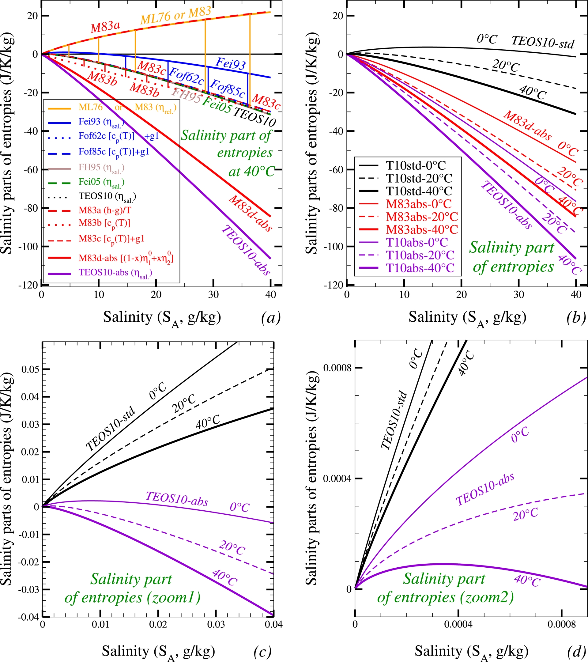
The three Feistel’s and TEOS10 curves labeled FH95, Fei05, and TEOS10 are clearly very close to each other in the Figure 1(a). The older formulation of Feistel (1993, in blue, labelled Fei93) differs from these three almost superimposed curves, with a positive bias (vertical blue thin lines) but with similar negative and decreasing values for SA > 10 g⋅kg−1.
This positive bias can be explained by the different arbitrary definitions made for the zero of enthalpies and entropies in both Fei93 and Feistel and Hagen (1994, hereafter FH94). This was recalled in FH95, where it was explicitly stated (p. 269) that the arbitrary choice made in Fei93 (and still retained in FH94) was to “define the enthalpy per salt particle to vanish at infinite dilution” (i.e., S = 0 PSU), and to arbitrarily decide from FH95 onwards “to set entropy and enthalpy to zero for the standard ocean statet = 0 °C, p = 0 MPa andS = 35 PSU” because “entropy per salt particle diverges when salinity goes to zero” in Fei93 and FH94.
I show in Table 5 a comparison of the lower-order terms (g[1;0;0] + g[1;1;0] y) x2 ln(x) + (g[2;0;0] + g[2;1;0] y) x2 for the Gibbs function gsw, which enter the entropy formula via 𝜂sw = −∂gsw/∂t = − (1/40)∂gsw/∂y, and thus via − (1/40)[g[1;1;0] x2 ln(x) + g[2;1;0] x2]. If the varying coefficient g[2;0;0] only concerns the enthalpy, the other varying coefficient g[2;1;0] impacts the value of the seawater entropy, and Fei93’s value is indeed very different from those for FH95, Fei05, and TEOS10, with a large impact on the seawater entropy via the term − [g[2;1;0]/1.6](SA/1000). This means from (23) that the changes in −g[2;1;0]/1.6 correspond to those in 𝜂s0 −𝜂w0 computed at 0 °C. The difference of about 160.9 + 615.7 = 776.6 between Fei93’s and FH95’s formulations corresponds to a change in 𝜂s0 −𝜂w0 of about −485.7 J⋅K−1⋅kg−1, and from (23) to a change in 𝜂sw/sal.(t,SA) of about −19.4 J⋅K−1⋅kg−1 at SA = 40 g⋅kg−1, which is in agreement with Figure 1(a) and with the same vertical shift of about −19.4 J⋅K−1⋅kg−1 (from −12.164 to −31.561) between Fei93’s and FH95’s curves.
The low-order Gibbs’ coefficients g0 = g[1;0;0], g1 = g[1;1;0], g[2;0;0] and g[2;1;0] involved in Feistel’s relationships in the terms (g0 + g1y)x2 ln(x), g[2;0;0]x2 and g[2;1;0]x2 y for the non-dimensional variables x2 = SP/(40 g⋅kg−1) or x2 = SA/(40.188617 g⋅kg−1) and y = t/(40 °C)
| g[2;0;0] | g[2;1;0] | g[1;0;0] | g[1;1;0] | |
|---|---|---|---|---|
| Feistel (1993, Fei93) | [−4204.5207] | [−615.7087] | 5814.9808 | 851.5440 |
| Feistel and Hagen (1995, FH95) | (1531.9856) | (160.9033) | 5813.3468 | 851.3047 |
| Feistel (2003; 2005, Fei05) | (1376.280…) | (140.577…) | 5813.287… | 851.2959… |
| McDougall, Feistel, et al. (2010, TEOS10) | (1416.276…) | (168.072…) | 5812.815… | 851.2267… |
The Millero curves (ML76 or M83) plotted in orange on Figure 1(a) show an even greater vertical shift, with values made positive and increasing for all values of SA. We could try to interpret this increased shift relative to the curves of Fei93, FH95, Fei05, and TEOS10 as a result of the absolute definitions of reference entropies a priori included in ML76 and M83. However, the impact of these absolute definitions is negative when using the formula (20) established above for Δ𝜂s, as shown by the differences between the black curve for TEOS10 (standard) and the purple curve for TEOS10-abs. It therefore becomes important to be able to explain the reasons for such unusual features for the impacts in ML76 and M83 of the absolute definitions of reference entropies.
It can first be noted that the orange and increasing curve for ML76 or M83 has already been plotted by Sharqawy et al. (2010, Eq. (44), p. 373, Figure 16, p. 374) and Qasem et al. (2023, Figure 5.1, p. 125), who already showed that all other “specific salinity” curves plotted from Chou (1968), Pitzer et al. (1984), Levelt Sengers and Dooley (1992, IAPWS), Sun et al. (2008), Cooper and Dooley (2008, IAPWS), and Nayar et al. (2016) were decreasing with the salinity SA. This means that the increasing orange curve for ML76 + M83 in Figure 1(a) is truly atypical, as it differs from all the others (Chou, 1968; Pitzer et al., 1984; Levelt Sengers and Dooley, 1992; Feistel, 1993; Feistel, 2003; Feistel, 2005; Sun et al., 2008; Cooper and Dooley, 2008; McDougall, Feistel, et al., 2010; Nayar et al., 2016). Conversely, the decreasing black curve for TEOS10 (standard), which I relied on in my paper, is very similar to all the others except those by Millero.
In fact, it can be shown that the formulations proposed by ML76 (Eq. (136), p. 1072) and M83 (Eq. (147), p. 36) corresponding to the curves in orange (ML76 or M83) do not include the absolute values of the reference entropies. Indeed, they do not correspond to the definitions (21) and (22) leading to the saline parts (23) for the entropy of seawater. In order to prove this, it can be noted that the plot of the curve M83a (in bold dashed red) for the quantity (h − g)/T is superimposed on that of the entropy 𝜂 (ML76 + M83), with h the enthalpy and g = h − T 𝜂 the Gibbs function previously defined both in ML76 (Eq. (67), p. 1050 and Eq. (118), p. 1068) and M83 (Eqs. (54)–(57), p. 15–16 and Eqs. (126)–(129), p. 32). These definitions were derived long before the absolute liquid-water and sea-salt entropies $\overline{\eta }_1^{\circ }$ and $\overline{\eta }_2^{\circ }$ were respectively defined in ML76 (p. 1070–1072) and M83 (p. 34–35)9 . This confirms that neither ML76, M83, or M83a can represent the absolute version of the saline part of seawater entropy.
In order to continue the investigation, it is possible to start from the definition of the specific heat of seawater expressed in ML76 (Eqs. (52), p. 1044) and M83 (Eqs. (34)–(37), p. 11) as
| \begin {eqnarray} c_{p\mathrm {sw}}(t,S) &=& c_{p0}(t) + A_{{c}p}(t)\, S + B_{{c}p}(t) \, S^{3/2}. \label {Eq_M83_Cpsw}\end {eqnarray} | (24) |
| \begin {eqnarray} A_{{c}p}(t) &=& -7.644 + 0.10727\, t - 1.38 \times 10^{-3} t^2, \label {Eq_M83_Acp}\end {eqnarray} | (25) |
| \begin {eqnarray} B_{{c}p}(t) &=& 0.177 - 4.08 \times 10^{-3} t + 5.35 \times 10^{-5} t^2, \label {Eq_M83_Bcp}\end {eqnarray} | (26) |
| \begin {eqnarray} c_{p0}(t) &=& 4217.4 - 3.720283\, t + 0.1412855\, t^2 + 2.654387 \times 10^{-3} t^3 + 2.093236 \times 10^{-5} t^{4\!}. \label {Eq_M83_cp0} \end {eqnarray} | (27) |
The next step is to define a value of the seawater entropy by integrating cpsw(t)/(t + 273.15) up to an arbitrary function of salinity 𝜂0 only, and independent of the temperature. This leads, with 𝜂0(0 °C) = 0, to the red dotted curve M83b, with a small negative bias with respect to the FH95, Fei05, and TEOS10 curves (thin vertical red lines).
This small negative bias of the curve M83b is clearly reduced with the red curve M83c plotted with the following alternative choice for 𝜂0(0 °C), obtained by adding the impact of the Gibbs ideal-solution term g1x2 ln(x)y with the value g1 = g[1;1;0] ≈ 851.3 typical of FH95 + Fei05 + TEOS10, for which the impact on entropy is − [(851.3/1600)ln(S/40)]S > 0 for 0 < S < 40, and null for S = 0 and S = 40. The same method can be used by integrating the values of cpsw(t)/(t + 273.15) published in the earlier articles of Fofonoff (1962, Eqs. (29)–(30)–(31), p. 13–14)) and Fofonoff (1985, Table-7, p. 3339), with the blue curves Fof62c and Fof85c obtained by adding the same term − (g1/40)x2 ln(x) with g1 ≈ 851.3 as for M83c.
As a result, all curves for Fof62c, M83c, Fof85c, FH95, Fei05, and TEOS10 almost overlap in Figure 1(a). This means that the ML76 + M83 formulation of cpsw(t,S) recalled in (24) is relevant, and that the atypical behavior of the M83 and M83b curves must correspond to a deeper difference in the functions h, g = h − T 𝜂 and 𝜂 defined in these papers. Furthermore, Feistel (1993, p. 102–103) indicates that several problems exist in the previous Millero’s formulations (forming parts of what he called the “EOS80” system of equations): “…there is a numerical mismatch in the paper of ML76, in transforming heat capacity to apparent molal heat capacity in the form of a generalized Debye–Hückel formula. Because this formula is used later to compute enthalpy and free enthalpy (and thus entropy), the temperature dependence of both is inconsistent with heat capacity. …theory predicts the power series in salinity would begin with$S\, \sqrt{S}$ in the case of relative enthalpy and withS ln(S) in the case of relative free enthalpy (and thus of entropy). The corresponding functions reported are smoothed out at small salinities to begin simply with S. Therefore they cannot be used correctly to compute, say, the chemical potential (and thus the entropy). …while density etc. are defined in absolute terms, thermal properties are only given relative to an infinitely diluted reference state. It is not obvious how these quantities have to be combined correctly if necessary, for example when computing the chemical potential (and thus the entropy). ‘‘Relative” means thatG(S,t,p) is zero at the infinite dilution reference state, where all ion-ion interactions are neglected at temperaturet = 0 °C (T = 273.15 K) and pressurep = 0 bar (P = 1 atm).”
Indeed, it turns out that the ML76 and M83 definitions of “relative” and “relative apparent” parts of any extensive quantity S (like the heat content or enthalpy, the volume, the available enthalpy or Gibbs function, and the entropy noted S) are the same as those published in the previous paper by Millero, Hansen, et al. (1973), and in fact go back to the older books by LR61 and Harned and Owen (1958; 1950; 1943). The “relative” feature means considering only the deviations Srel. = S − S° from the molar or specific actual value S = n1S1 + n2S2 and the “infinite-solution” value $S^{\circ } = n_1 S^{\circ }_1 + n_2 S^{\circ }_2$. They are both computed for the actual n1 moles of liquid water and n2 moles of sea salts, and with the “infinite-solution” values $S^{\circ }_1$ and $S^{\circ }_2$ corresponding to n2→0 and thus SA→0. It is thus clear that the omission of a function S° for entropy—which varies with salinity—renders this “relative” view of entropy, defined by S(t,SA,p) − S°(t,SA,p), somewhat meaningless for the study of the entropy function S(t,SA,p). This is why Chou (1968, Eq. (5)–(9), p. 96) defined the specific entropy of a solution consisting of n1 mole of water and n2 moles of salt as $s = n_1 \, \overline{s}^{\circ }_1 + n_2\, \overline{s}^{\circ }_2 + (\cdots )$, therefore including the term $n_1 \, \overline{s}^{\circ }_1 + n_2\, \overline{s}^{\circ }_2$ not included in Millero’s “relative” formulations. Similarly, Pitzer et al. (1984, Eq. (1), p. 3) defined the Gibbs function of the real system as $G = n_1 G^{\circ }_1 + n_2\, \overline{G}^{\circ }_2 + (\cdots )$, again including the terms not included in “relative” Millero’s formulations.
Starting from (21) the “infinite-solution” and “relative” value of the seawater entropy (noted 𝜂) can be written as
| \begin {eqnarray} \eta _{\mathrm {sw}}^{\circ }(t,S_{\mathrm {A}}) &=& \left (1-\frac {S_{\mathrm {A}}} {1000}\right ) \eta _{w}(t) + \left (\frac {S_{\mathrm {A}}}{1000}\right )\eta _{s}(t,S_{\mathrm {A}}=0), \label {Eq_eta_infinite_sol}\end {eqnarray} | (28) |
| \begin {eqnarray} \eta _{\mathrm {sw/rel.}}(t,S_{\mathrm {A}}) &=& \eta _{\mathrm {sw}}(t,S_{\mathrm {A}}) -\eta _{\mathrm {sw}}^{\circ }(t,S_{\mathrm {A}}), \label {Eq_eta_relat_1}\end {eqnarray} | (29) |
| \begin {eqnarray} \eta _{\mathrm {sw/rel.}}(t,S_{\mathrm {A}}) &=& \eta _{w}(t) + \left (\frac {S_{\mathrm {A}}}{1000}\right ) \times [\eta _{s}(t,S_{\mathrm {A}}) - \eta _{s}(t,S_{\mathrm {A}}=0)]. \label {Eq_eta_relat_2} \end {eqnarray} | (30) |
It therefore appears that the so-called “relative” entropy of ML76 and M83 is very different from the salinity parts studied in Fei93, FH95, Fei05, and TEOS10, with the liquid-water entropy 𝜂w(t) in the last term of the salinity-part formula (23) replaced by the infinite-solution sea-salts entropy 𝜂s(t,SA = 0) in the “relative-entropy” formula (30), together with the additional first term 𝜂w(t).
According to ML76 (p. 1072) and M83 (p. 36), “Since future workers may wish to look at entropy surfaces in the oceans,” the “relative-entropy” formula was fitted to the function [h(t,S) − g(t,S)]/(t + 273.15) to give
| \begin {eqnarray} \eta _{\mathrm {sw/rel.}}(t,S) &=& A_s(t) S(\mbox {\textperthousand }) + B_s(t) S(\mbox {\textperthousand })^{3/2} + C_s(t) S(\mbox {\textperthousand })^{2}, \label {Eq_M83_s} \end {eqnarray} | (31) |
| \begin {eqnarray} A_s(t) &=& +1.42185 - 3.1137 \times 10^{-4} t + 4.2446 \times 10^{-6} t^2, \label {Eq_M83_s_A}\end {eqnarray} | (32) |
| \begin {eqnarray} B_s(t) &=& - 0.21762 + 4.1426 \times 10^{-4} t - 1.6285 \times 10^{-6} t^2, \label {Eq_M83_s_B}\end {eqnarray} | (33) |
| \begin {eqnarray} C_s(t) &=& + 1.0201 \times 10^{-2} + 1.5903 \times 10^{-5} t - 2.3525 \times 10^{-7} t^2. \label {Eq_M83_s_C} \end {eqnarray} | (34) |
| \begin {eqnarray} \eta _{\mathrm {sw/sal.}}(t,S_{\mathrm {A}}) &=& \eta _{\mathrm {sw}}(t,S_{\mathrm {A}}) -\eta _{w} (t), \label {Eq_eta_sal_2}\end {eqnarray} | (35) |
| \begin {eqnarray} \eta _{\mathrm {sw/sal.}}(t,S_{\mathrm {A}}) &=& \eta _{\mathrm {sw/rel.}} (t,S_{\mathrm {A}})+\left (\frac {S_{\mathrm {A}}}{1000}\right ) \times [\eta _{s}(t,S_{\mathrm {A}}=0)-\eta _{w}(t)]. \label {Eq_eta_sal_3} \end {eqnarray} | (36) |
To do so, the ML76 + M83 specific absolute reference sea-salt entropy is first recalled in (11). Then, the entropy of liquid water 𝜂w(t) was computed by ML76 (p. 1072) and M83 (p. 36) by first fitting the specific heat capacity cpw(t) given by (27) in terms of the absolute temperature T (K). This leads to
| \begin {eqnarray} c_{pw}(T) &=& 21.02343 \times 10^{3} - 119.8696\, T + 9.828769 \times 10^{-2} T^2 + 8.466352 \times 10^{-4} T^3 - 1.554175 \times 10^{-6} T^4, \label {Eq_M83_Cpw} \end {eqnarray} | (37) |
| \begin {equation} \eta _w(T) = \eta _w(25~\mbox {{\textdegree }C}) + \int _{298.15}^{T} \frac {c_{pw}(T')}{T'}\,\mathrm {d}T', \label {Eq_M83_S_w_int} \end {equation} | (38) |
| \begin {eqnarray} \eta _{w}(T) &=& [\eta _{w0}(25~\mbox {{\textdegree }C}) - 92.8218] + 21.02343 \times 10^{3} \ln (T) - 119.8696\, T + 4.914384 \times 10^{-2} T^2 + 2.822117 \times 10^{-4}T^3 - 3.885437 \times 10^{-7} T^4. \label {Eq_M83_Sw} \end {eqnarray} | (39) |
The next problem is that the entropy of sea salts 𝜂s(t,SA), depending on the temperature and salinity, is not calculated explicitly by ML76 or M83, like that 𝜂w(t) of liquid water in (39) and that relative 𝜂sw/rel.(t,S) for seawater in (31). However, the absolute value of the reference sea-salt entropy at infinite dilution 𝜂s0(25 °C) ≈ 1513.1 J⋅K−1⋅kg−1 recalled in (11) was explicitly calculated by ML76 and M83 at 25 °C. We can therefore imagine a first-order formulation to be used in (36) and based on (16), but valid for variable absolute temperatures T and based on the specific heat $\overline{C}_{p{s}} (25~ \mbox{{\textdegree }C}) \approx {-}1656~ \mathrm{J}{\cdot }\mathrm{K}^{-1}{\cdot }\mathrm{kg}^{-1}$ calculated in (15), leading to
| \begin {equation} \eta _{s}(t,S_{\mathrm {A}}=0) \approx \eta _{s0}(25~\mbox {{\textdegree }C}) + \overline {C}_{p{s}}(25~\mbox {{\textdegree }C}) \times \ln \left (\frac {T}{298.15}\right ).\raisebox {-1.1pc}{} \label {Eq_eta_s_0C_Marquet_2023_T_bis} \end {equation} | (40) |
This M83d-abs curve corresponds to the expected and hoped-for result, as it validates, in a way, the absolute definition of seawater entropy as I propose and have plotted with TEOS10-abs. The M83d-abs curve corrects the “relative” ML76 + M83 + M83a aspect that was too atypical and was not included in the subsequent IAPWS and TEOS10 projects, in which Millero has nevertheless participated since 1983. The difference between the M83d-abs and TEOS10-abs curves can probably be explained by the remaining approximations and imperfections in the ML76 and M83 formulations, as listed by Feistel (1993, p. 102–103) about the “EOS80” system of equations.
It should be noted that the decrease in entropy with salinity is more pronounced for absolute versions and is not contrary to the fact that entropy must increase during the process of dissolving salts in pure water. As an example, the process of dissolution of crystals of NaCl corresponds to a positive change in seawater entropy for the reaction NaClcr⟶(Na+)aq + (Cl−)aq. Indeed, the entropy for a crystal of NaCl is 72.14 J⋅K−1⋅mol−1, whereas the entropy for the separate ions (Na+)aq and (Cl−)aq is 59.00 + 56.36 = 115.36 J⋅K−1⋅mol−1. This leads to an increase of entropy of 115.36 − 72.14 = +43.22 J⋅K−1⋅mol−1, representing the impact on the entropy of the dissolution of the NaCl crystal. In fact, the decrease in absolute entropy with salinity must be interpreted differently: it is as a decrease in the average entropy per unit mass when a mass of water with a higher salinity is added to another with a lower salinity, with the salts already dissolved in both masses of water. For such a process the entropy decreases because the reference entropy of ocean salts (1513.1 J⋅K−1⋅kg−1) is smaller than that of liquid water (3885.65 J⋅K−1⋅kg−1). In this sense, the errors in the tuning leading to the ML76 and M83 “relative” formulation had to be corrected in the present formulation based on the amended version of TEOS10, with, moreover, the use of the absolute values of the reference entropies.
The second plot in Figure 1(b) shows the joint variations with the salinity of the curves 𝜂sw(t,SA) for a selection of three temperatures: t = 0 °C, 20 °C, and 40 °C. We can see that the behaviors observed at 40 °C remain unchanged at other temperatures, with a more noticeable decrease in all cases in Figure 1(b–d) for the absolute versions of the entropies.
Finally, the impact of the term x2 ln(x) in the TEOS10’s entropy formulation corresponding to the term SA ln(SA) introduced by Onsager and Fuoss (1932, Eq. (1.1.2), p. 2689) is to create a vertical tangent at the origin. This is particularly visible in Figure 1(c) and (d), where I show that this behaviour starts to exist only for SA much smaller than 1 g⋅kg−1. Differently, a general decrease of the absolute entropy exists for the whole oceanic range of salinity from 5 to 40 g⋅kg−1.
3.2. The temperature-salinity (t − SA) diagram
The same results are obtained with the study of the other temperature-salinity (t − SA) diagram plotted in the Figure 2. The green lines are for constant values of the TEOS10 potential-density anomaly10 (𝜎𝜃 =𝜌 𝜃 − 1000, in g⋅m−3). Using potential density instead of local density will make it easier to compare the density of points of vertical profile at different depths in the second part of the paper, always using the same family of green lines (surface, pr = 0).
The isopycnic potential-density anomaly (solid green) lines, the standard TEOS10 entropy (dashed black) lines, and the new absolute TEOS10 entropy (solid red) lines are plotted on a classical t − SA Temperature-Salinity diagram. The three red and black circles represent isentropic processes (see the main text).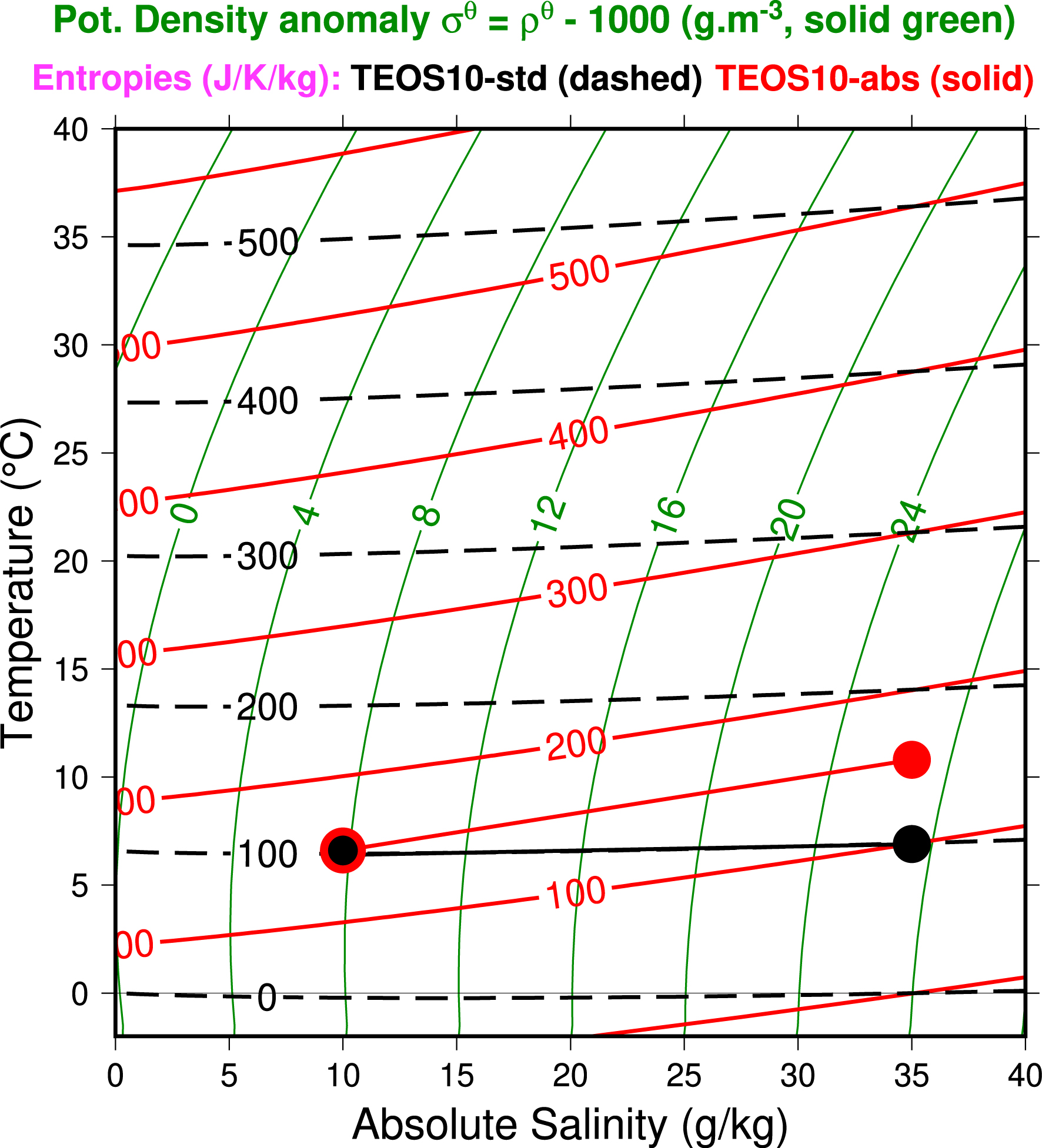
In this t − SA diagram, the new absolute seawater entropy red lines are different from the standard TEOS10 black lines: the new absolute values increase with the salinity, whereas the standard TEOS10 values are almost constant (especially for the smaller values of salinity and temperature). Similar differences (not shown) exist between the standard and absolute versions of the seawater entropy plotted with the entropy-temperature diagram published in Feistel, Wright, Kretzschmar, et al. (2010, Figure 4, p. 103).
Three black and red circles are plotted to show the differences in temperature associated with an isentropic process starting at about 6.6 °C and with a change in salinity from 10 to 35 g⋅kg−1: the change in temperature is about 4 °C greater for the absolute version than for the standard TEOS10 version (Δt ≈ +0.3 °C compared with +4.2 °C). This difference is significant, as shown by the applications to real cases described in Part II.
It should be noted here (like in Part II) that the term “isentropic” (or same entropy) includes possible joint variations in pressure, temperature, and salinity, without prejudging any adiabatic (no exchange of heat) or closed (same salinity) aspect of the evolution of ocean parcels. This is analogous to the definition of “isopycnal” processes, where density (or potential density) remains constant regardless of joint variations in pressure, temperature, and salinity, with variations in temperature and salinity along isopycnals described with spiciness.
3.3. General impacts of the third law in physics
It may be important to recall the first validations for H2, Ar and Hg made close to 0 K and recalled by Nernst (1926, p. 185–186) for the Sackur–Tetrode–Planck absolute entropy constants defined and studied by Planck (1917), Nernst (1918; 1921) and Planck (1921). These authors showed that the theoretical and statistical-quantum absolute value C0 ≈−1.61 was in agreement with the experimental and calorimetric third-law value C0 ≈−1.62 ± 0.03. This justified and allowed the computation of the saturation pressures from the third-law absolute entropies if the latent heats are known (see Section 12.1 in the SM).
It is possible to show another modern validation of the theoretical and calorimetric third-law absolute values computed at 0 °C for the water-vapour and ice-Ih entropies. I have first computed (see Section 4.6 and Eq. (126) in the SM) the third-law statistical-quantum water-vapour entropy
| \begin {equation} \eta _{v/\mathrm {3rd}}^{\mathrm {stat.}}(T_0,p_0) \approx 10317.9 \pm 0.63~\mathrm {J}{\cdot }\mathrm {K}^{-1}{\cdot }\mathrm {kg}^{-1} \label {Eq_Entropy_H20_vap_stat} \end {equation} | (41) |
| \begin {equation} \eta _{i/\mathrm {3rd}}^{\mathrm {calor.}}(T_0) \approx 2295.5 \pm 1.9~\mathrm {J}{\cdot }\mathrm {K}^{-1}{\cdot }\mathrm {kg}^{-1}. \label {Eq_Entropy_H20_ice_calor} \end {equation} | (42) |
(a) The specific heat at constant pressure cp(T) for H2O (Ice-Ih) for absolute temperatures T from 0 K to T0 = 273.15 K. (b) The absolute entropies for H2O (Ice-Ih, liquid and vapour) from 0 K to 340 K, with the calorimetric values $\eta _0 +\int _0^T c_p(T')\, \mathrm{d}\, \ln (T')$ (solid red lines) including the Pauling–Nagle residual entropy 𝜂0 ≈ 0.189 kJ⋅K−1⋅kg−1 at 0 K, and the statistical values 𝜂 = k ln(W) (dashed blue line) automatically taking into account the residual entropy at 0 K and the latent heat of sublimation Lsub(T0) ≈ 2834.5 kJ⋅kg−1 at 273.15 K. The term 𝛿𝜂 ≈ 10.318 − 2.295 = 8.023 kJ⋅K−1⋅kg−1 (green arrow) is the difference between the statistical water-vapour and calorimetric Ice-Ih absolute entropies at T0 = 273.15 K.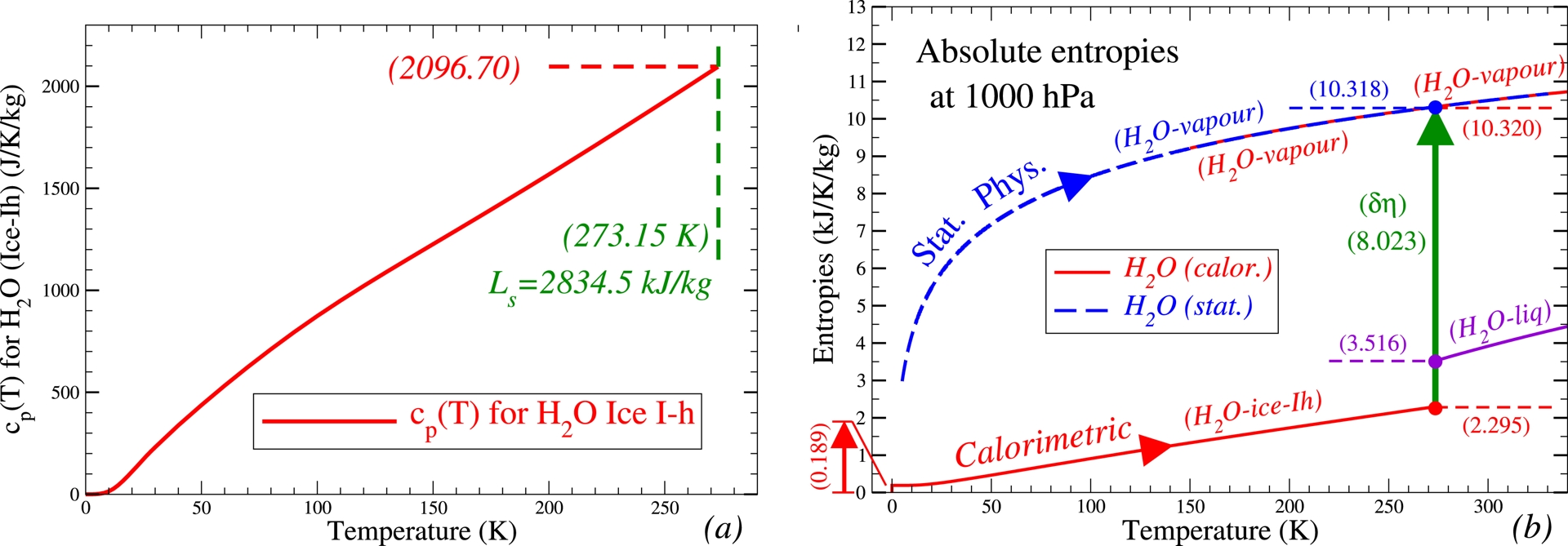
As a consequence, a new validation of the third law of thermodynamics can be obtained by computing (see Section 3.5 and p. 19 in the SM) the calorimetric water-vapour entropy at T0 = 273.15 K and p0 = 105 Pa via the relationship
| \begin {eqnarray} \eta _{v/\mathrm {3rd}}^{\mathrm {calor.}}(T_0,p_0) &=& \eta _{i/\mathrm {3rd}}^{\mathrm {calor.}}[T_0, p_{\mathrm {sat}} (T_0)] + \frac {L_{\mathrm {sub}}(T_0)}{T_0} - R_{v}\,\ln \left [ \frac {p_0}{p_{\mathrm {sat}}(T_0)}\right ] \approx 10320 \pm 4~\mathrm {J}{\cdot }\mathrm {K}^{-1}{\cdot } \mathrm {kg}^{-1}, \label {Eq_Entropy_H20_vap_calor} \end {eqnarray} | (43) |
Conversely, one can use (41) and (42) to calculate either the latent heat of sublimation Lsub(T0) or the saturation pressure psat(T0) variable from the other variable and from the difference in third-law entropies
| \begin {eqnarray} \delta \eta (T_0,p_0) &=& \eta _{v/\mathrm {3rd}}^{\mathrm {stat.}} (T_0,p_0) - \eta _{i/\mathrm {3rd}}^{\mathrm {calor.}}[T_0, p_{\mathrm {sat}}(T_0)] \approx 8022.4 \pm 2.6~\mathrm {J}{\cdot }\mathrm {K}^{-1}{\cdot } \mathrm {kg}^{-1} \label {Eq_delta_Entropy_H20} \end {eqnarray} | (44) |
| \begin {eqnarray} L_{\mathrm {sub}}(\delta \eta , p_{\mathrm {sat}}, T_0, p_0) = T_0 \left \{\delta \eta (T_0,p_0) + R_{v}\,\ln \left [\frac {p_0} {p_{\mathrm {sat}}(T_0)}\right ]\right \}\label {Eq_H20_Ls_T0} \end {eqnarray} | (45) |
| \begin {eqnarray} p_{\mathrm {sat}}(\delta \eta , L_{\mathrm {sub}},T_0, p_0) = p_0 \exp \left [\frac {\delta \eta (T_0,p_0)}{R_{v}} - \frac {L_{\mathrm {sub}} (T_0)}{R_{v} T_0}\right ] \label {Eq_H20_Psat_T0} \end {eqnarray} | (46) |
These calculations show the predictive power of the statistical (for water vapour) and calorimetric (for Ice-Ih) third-law independent computations leading to the blue and red disks, respectively. These calculations form a validation of the physical significance of the third-law values of the entropy by forming a little-known link between the numerical values of Lsub(T0) and psat(T0), which are generally considered to be independent experimental constants. This creates an unexpected third-law implicit impact on the thermodynamic conditions at the surface of the oceans and thus impacts the measurable evaporation processes.
Incidentally, these calculations may also provide a justification for and a physical interpretation of the residual entropy of 189 J⋅K−1⋅kg−1. Indeed, if we subtract this value from the absolute entropy of ice, then according to (44), the quantity 𝛿𝜂(T0,p0) increases from about 8023 to about 8212 J⋅K−1⋅kg−1, resulting in, according to (45) and (46), the unrealistically high values of Lsub(T0) ≈ 2885.7 kJ⋅kg−1 and psat(T0) ≈ 917.6 Pa in comparison with the experimental values of Lsub(T0) ≈ 2834.5 ± 0.5 kJ⋅kg−1 and psat(T0) ≈ 611.15 ± 0.10 Pa. The bias of 189 × 273.15 ≈ 51.6 kJ⋅kg−1 for Lsub(T0) and the multiplicative factor of exp(189/461.65) ≈ 1.506 for psat(T0) are indeed unrealistic values. This means that it was not possible to separate the residual value from the absolute calorific entropy of ice-Ih, as suggested by Feistel (2019) who tried “Distinguishing between Clausius, Boltzmann and Pauling entropies of frozen non-equilibrium states.” This also means that this quantity, 189 J⋅K−1⋅kg−1, is likely hidden somewhere in the quantum-statistical calculations carried out by Sackur, Tetrode, Planck, and others for the translational, rotational, and vibrational degrees of freedom of atoms and molecules.
Moreover, I recall in Section 12.2 of the SM that the equilibrium constants of chemical reactions K(T) ultimately depend on the absolute entropies S0 of the reactants and products, via the well-known stability relationship ΔGr = ΔHr − TΔS0 = −RT ln(K). General forms like ln(K) = ΔS0/R −ΔHr/(RT) = A + B/T + C ln(T) are considered both in ozone chemistry (NASA-JPL publication by Burkholder et al., 2020) and seawater chemistry, where it was calculated in Weiss (1974) by adjustments to the observed data. They are also considered, for instance, by Millero (1995) for the study of carbon dioxide concentration in the oceans and more generally described in the DOE (1994) publication. In the general form above, the third-law absolute entropies of reactants and products must impact the constant term A. I show in Section 12.2 of the SM such an impact for the atmospheric reactions Cl + O2 ⟷ ClO2 and NO + NO2 ⟷ N2O3 and the seawater reaction $\mathrm{HCO}_3^- \longleftrightarrow \mathrm{H}^+ + \mathrm{CO}_3^{2-}$ (ionization of the bicarbonate anion). The constant terms A can be computed from the theoretical or experimental values of the third-law absolute entropies of molecules, anions, and cations acting as reactants and products. Therefore, the concentrations of ozone in the atmosphere and of sea salts in the oceans both depend on the third-law absolute reference entropies as those considered in the present paper, in Millero’s papers, and in some few others in atmospheric science (like Hauf and Höller, 1987; Marquet, 2011, …), via the photochemistry of the stratosphere and the electrolytic chemistry of the oceans. This is how the absolute values of the entropies influence the observed values of the concentrations of ozone and sea salts, where the concentrations vary with the temperature and pressure. This influences, in return and via the interactions with the radiations, the vertical profiles of the temperature, which is an obvious observable quantity.
Moreover, I show in Section 12.9 of the SM that similar impacts exist for the turbulence acting on the observable temperature-like variables. This, according to Richardson (1919; 1922), should be calculated via a turbulent mixing acting on the absolute entropy variable and not on the temperature variable (see the Section “A need to update the seawater entropy”). I show in Section 12.9 of the SM that the Lewis number (ratio of the thermal and water exchange coefficients) is different from unity for the moist-air absolute entropy variable 𝜃s (Marquet, 2011), for which Ks > 0. This generates a counter-gradient term for the usually used liquid-water potential temperature 𝜃l variable (Betts, 1973), for which Kh does not even have a definite sign. This means that the vertical and horizontal structures of temperature must ultimately depend on the absolute definition of the difference in entropy (like svr − sdr for the atmosphere and 𝜂s0 −𝜂w0 in the ocean) and the corresponding absolute-entropy exchange coefficients. Accordingly, it is possible to make a link between these atmospheric turbulent phenomena and those in the oceans. Indeed, several of the parameterizations are based on the principle of “double diffusion,” first studied by Stern (1960) for the “Salt-Fountain” and still considered in Ma and Peltier (2024) for the polar oceans. Here, the exchange coefficients are different for the large-scale velocity (momentum), heat (temperature), and salinity, respectively (see, for instance, Canuto et al., 2002).
Moreover, in order to comply with Richardson’s requirements, an equivalent of the atmospheric variable 𝜃s = T0 exp[(s − sd0)/cpd] (Marquet, 2011; Marquet and Stevens, 2022) to be used in turbulent schemes of oceanic simulations could be defined as the seawater absolute-entropy (potential?) temperature 𝜃𝜂 derived from the value of the absolute entropy 𝜂abs given by (18), (19), and (20), but rewritten as 𝜂abs = cw ln(𝜃𝜂/T0), and thus with 𝜃𝜂 = T0 exp(𝜂abs/cw)written as
| \begin {eqnarray} \theta _{\eta } &=& 273.15 \times \exp \left (\frac {\eta _{\mathrm {std/ TEOS10}}}{4218}\right ) \times \exp \left [(-0.446 \pm 0.004) \left (\frac {S_{\mathrm {A}}- S_{\mathrm {SO}}}{1000}\right )\right ], \label {eq_theta_eta_new} \end {eqnarray} | (47) |
I show in Figures 42 to 44 in Section 12.9 of the SM that 𝜃 and Θ remain very close to each other for several arctic and tropical CTD profiles (up to ± 0.03 °C). The differences between the actual temperature T and both 𝜃 and Θ are also small close to the surface (up to ± 0.03 °C for depths smaller than 250 dbar), where the impact of salinity on 𝜃𝜂 is the largest and can reach ± 1.5 °C. Note the interesting feature that 𝜃𝜂 becomes similar to both 𝜃 and Θ for layers deeper than 3000 dbar (up to ± 0.04 °C), where the differences with T can reach −0.6 °C. These numerical evaluations confirm the potential of the 𝜃𝜂 variable to become a kind of thermal variable on which ocean turbulence is acting and becoming a kind of “absolute seawater potential temperature”. This variable 𝜃𝜂 is numerically similar to 𝜃 and Θ in deeper layers, but different from them in the mid and surface layers. This simply means that the seawater entropy (and thus 𝜃𝜂) is very likely the more natural conservative variable.
In addition to the examples in Section 3.1 concerning the unexpected links between latent heat and the saturation pressure of water vapour, the examples described in this section show that there are observable impacts in geophysics of the absolute reference entropy values, thereby providing a physical meaning for calculations and studies of absolute seawater entropy. However, the same doubts concerning the physical relevance of absolute entropy will continue to exist in atmospheric and oceanic sciences, much like doubts can still exist for the ultimate realism of the principles of many general principles of physics, such as the existence of the Michelson–Morley–Lorentz–Einstein’s limiting velocity (c) of physical phenomena in a vacuum or the existence of the Planck’s quantum of action (h). Indeed, there is no demonstration in the logical, mathematical, or physical senses of these facts, which are simply observed, never disproved, and therefore elevated to the status of general principles. The same applies to the third law and the principle of unattainability of the absolute zero of temperature, subject to amending Planck (1911; 1917) formulation by adding possible residual entropies at 0 K in the calorimetric computations for some species like H2O, as logically included in 𝜂abs and 𝜃𝜂 for seawater.
Accordingly, other contributions than TEOS10 have admitted the possibility of at least considering as an option the absolute entropies for liquid water and dry air (ML76, M83, Feistel and Hagen, 1995; Lemmon et al., 2000; Feistel and Wagner, 2006). Nonetheless, it is often still considered that the TEOS10’s choice is consistent with the first conclusion of the 5th International Conference on the Properties of Steam in London (5th-ICPS et al., 1956). Indeed, this conference recommended (p. 1/30–1/32 and 3/34) that the specific internal energy and the specific entropy of the liquid water should be set equal to zero at the triple point temperature of 0.01 °C instead of 0.00 °C, without affecting any measurable thermodynamic properties of the climate system. However, I show in Section 12.5 and Figure 32 of the SM that this first 1956 recommendation (p. 3/34) was only valid for the case of a pure liquid-water steam system. It was not valid for a mixture involving other species, like in the moist-air atmosphere and the seawater. Moreover, it was decided at the same time (ibid., p. 3/35–3/37) that the absolute values for the entropy of liquid water (computed from hypotheses made at 0 K) should also be mentioned in all subsequent studies. This is precisely what I have achieved in the present study by defining both 𝜂abs and 𝜃𝜂 for seawater, including the impacts of absolute and non-arbitrary definitions for both pure liquid-water and sea-salt reference entropies.
4. Conclusion
I have shown that several problems unfortunately prevent the direct use of the “relative” entropy formulation considered by Millero in 1976 and 1983. In particular, this Millero’s “relative” entropy formulation did not really take into account the absolute values of entropies and has never been considered since then, and in particular in IAPWS and TEOS10 formulations. For these reasons, I have based the present approach on the more modern formulation of TEOS10, with the sole addition of the absolute seawater entropy increment Δ𝜂s given by (18) proportional to both 𝜂w0 −𝜂s0 and SA − SSO, with the numerical value given by (20).
The existing standard TEOS10’s standard entropy formulation $\eta _{\mathrm{std/TEOS10}} = \eta ^{W}_{\mathrm{Fei03}}+\eta ^{S}_{\mathrm{Fei08}}$ is recalled in Tables 1 and 2. The reference entropies at 25 °C for pure liquid water (𝜂w0) and sea salts (𝜂s0) previously considered by Millero have been updated and computed at 0 °C from more recent and complete thermodynamic datasets to give the values (9) and (17). This is based on the third law expressed by Planck (1911; 1917), who generalized the heat theorem of Nernst (1906). Note that the residual entropy computed by Pauling (1935) and Nagle (1966) is automatically taken into account in the translational part of the entropy for liquid water, as it should be and as recalled by Feistel and Wagner (2005; 2006).
Therefore, the present paper offers the possibility of easily amending, if needed, the current standard formulation of TEOS10 to calculate the seawater absolute entropy corresponding to the recommendations of the third law of thermodynamics.
As a result, the entropy diagrams in Figure 1 show large differences in magnitude (and even signs) for the changes in seawater entropy as far as the salinity is not a constant. It should be worth adding the increment term Δ𝜂s wherever salinity values are particularly low or high and wherever salinity gradients are large. I show in the second part of the paper several examples from observations and analysed datasets where new isentropic features are revealed only with the absolute entropy of seawater. This might convince the oceanographic community, which believes that these differences have no physical significance, of the interest of the third law of thermodynamics.
Since the correction term Δ𝜂s depends on salinity and thus varies not only spatially but temporally, the calculation of entropy itself is changed beyond the addition of a simple constant (like 𝜂w0 in $\eta ^{W}_{\mathrm{Fei03}}$ recalled in Table 1). Consequently, because studies of the type “maximum entropy state” defined by d𝜂 = 0 depend on a certain combination of the differentials dT and (𝜂w0 −𝜂s0) dSA, there is an impact of the absolute reference entropy terms for non-stationary states with both dT≠0 and dSA≠0. This may generate impacts, for example, on regional, seasonal, and climate changes.
Furthermore, insofar as the seawater entropy gradient regions influence the turbulent transport of this thermodynamic state variable, with turbulent flows that must cancel out in isentropic regions, the absolute definition of seawater entropy should impact the second principle of thermodynamics.
Increased accuracy could be achieved by readjusting the tuning of the TEOS10’s formulation by using the absolute values of both 𝜂w0 and 𝜂s0 at 0 °C, rather than using the values g010 and g210 as free adjustment variables in Tables 1 and 2. Nonetheless, I think that adding the missing first-order correction term Δ𝜂s, as done by Millero and the present paper as well, does not introduce major uncertainties. This is due to the fact that the majority of the nonlinearities have already been considered in the well-founded standard TEOS10 version.
Since Fofonoff (1962, p. 8), the prevailing view in the oceanographic community is that the choice of the linear salinity function a2 + a4 S entering into the TEOS10 definition of the seawater entropy has no practical impact on known oceanographic applications and that the choice of fixing a2 and a4 is a matter of convention. However, some people think that the Millero and TEOS10 approaches may be considered valid and that neither should be subject to general rejection. It is within this last absolute-entropy framework that the present and Millero’s papers are situated, in line with the previous books of Fowler (1929), Guggenheim (1933), and Guggenheim (1950), where the third law of thermodynamics and the Sackur–Tetrode translational entropy were fully considered. Note, however, that Guggenheim rather called the absolute value of entropy the “conventional” entropy.
Feistel (2019) has recently decided to take the debate to the related subject of the physical meaning of the residual entropy of ice at 0 K. This is a subject that is different from the translational, quantum degrees of freedom and the absolute (or not) status of entropy. This subject of residual entropy only concerns a few species such as H2O, N2O, and CO, for which proton disorder still exists at 0 K. In any case, it is clear that only by taking into account the residual entropy for H2O computed by Pauling (1935) and Nagle (1966) can the calorimetric and quantum calculations of absolute entropy coincide, as shown in the Figure B1 of Marquet and Stevens (2022) and as taken into account in all thermodynamic tables (for instance, in Lewis and Randall, 1961; Chase, 1998; Atkins and de Paula, 2014; Schmidt, 2022; Atkins, de Paula and Keeler, 2023). Moreover, in Section 3.3 I provide evidence that this residual entropy impacts the relationships (45) and (46), with the values of latent heat and saturated pressure becoming unrealistic if this residual value is not taken into account.
For my part, I have complete confidence in these third-law thermodynamic tables that provide the absolute entropies. For the more general case of a mixture of variable composition like seawater, and as shown in this study, there is no reason to continue to apply only the first pure liquid water arbitrary recommendations expressed (p. 3/34) at London during the 5th-ICPS et al. (1956). It is needed to consider instead the next recommendation (p. 3/35-37), about the need to compute and study the absolute version of the entropy. Moreover, the residual entropies are small quantities and should not overshadow the much more fundamental aspect of the absolute values of the entropies due to the impact of the translational degrees of freedom of atoms and molecules, as calculated by Sackur, Tetrode, and Planck in the years 1911 to 1917.
It is true that most observable thermodynamic quantities do not depend on reference values of pure-water and sea-salt entropy (specific volumes, heat capacities, expansion coefficients, sound speeds, osmotic pressure, etc). But these reference values impact at least the seawater entropy itself, which deserves to be calculated and studied as one of the major thermodynamic state functions. This is confirmed by the interesting features revealed by the present study and the next part II.
Acknowledgments
I would like to thank the late Prof. Geleyn for his initial interest and discussions about the absolute definitions of entropy in the geophysical sciences.
The TEOS10-GSW Oceanographic FORTRAN software has been downloaded from https://www.teos-10.org/software.htm (McDougall and Barker, 2011).
The author would like to thank the anonymous referees and the editor for the constructive comments, which help to improve the manuscript.
Declaration of interest
The author does not work for, advise, own shares in, or receive funds from any organization that could benefit from this article, and has declared no affiliations other than their research organization.
Supplementary data
Supplementary materials are provided in the Zenodo file Marquet (2025).
1 In the studies of Marquet (2011; 2014), Marquet and Geleyn (2015), Marquet (2017), Marquet and Dauhut (2018), Marquet and Bechtold (2020), Marquet, Martinet, et al. (2022) and Marquet and Stevens (2022).
2 In particular: Kelley (1932), Latimer, Pitzer, et al. (1938), Rossini et al. (1952), Laidler (1956), Lewis and Randall (1961), Robinson and Stokes (1970), Robie et al. (1978), Wagman et al. (1982), Grenthe, Fuger, et al. (1992), Gokcen and Reddy (1996), Chase (1998), Atkins and de Paula (2014), Grenthe, Gaona, et al. (2020) and Atkins, de Paula and Keeler (2023).
3 For instance, in the contributions by Iribarne and Godson (1973; 1981), Emanuel (1994), Romps (2008), Pauluis et al. (2010), Raymond (2013) and Mrowiec et al. (2016), among so many others, for the atmosphere, and in the contributions by Fofonoff (1962), Fofonoff (1985), Feistel (1993), Feistel and Hagen (1995), Wagner and Pruss (2002), Feistel (2003), Warren (2006), Feistel, Wright, Miyagawa, et al. (2008), Sun et al. (2008), McDougall, Feistel, et al. (2010), …, up to Feistel (2019), McDougall, Barker, et al. (2023) and Feistel (2024), for the ocean.
4 TEOS10 in short for “Thermodynamic Equation Of Seawater - 2010.” See: http://www.teos-10.org/publications.htm.
5 It is of common use in oceanography to write the entropy with the symbols 𝜂 or 𝜎 (instead of the symbol S generally used in thermodynamics since Clausius, Boltzmann, and Planck) in order to keep the letters S, SP or SA for the salinity. Note that other symbols like 𝜙 are also used to denote the entropy, with, for instance, the T–𝜙 atmospheric diagram still called “Tephigram” in the UK and Canada.
6 I will refer in the present paper to the pages and numbers of figures, equations, and tables of the version of the TEOS10’s Manual downloaded in September 2024 from http://www.teos-10.org/pubs/TEOS-10_Manual.pdf.
7 Namely, as done in the part of the subroutine gsw_gibbs.f90 of the software GSW-Fortran-3.05-6 with the derivation options “(ns.eq.0).and.(nt.eq.1).and.(np.eq.0)”.
8 The corresponding correction term 4218 ×ln(273.15/298.15) ≈−369.39 J⋅K−1⋅kg−1 is about − 2 units smaller than the similar value − 367.36 J⋅K−1⋅kg−1 computed with the TEOS10’s (GSW) subroutine (liq_entropy_si), leading to a smaller TEOS10’s mean value $\overline{c_{w}} \approx 4194.6~ \mathrm{J}{\cdot }\mathrm{K}^{-1} {\cdot }\mathrm{kg}^{-1}$ between 298.15 K and 273.15 K and to a larger LR61 and ML76 pure-liquid water entropy of about 3518 J⋅K−1⋅kg−1 at 273.15 K.
9 Note that I have not used the notations s, S, $\overline{S}^{\circ }$, $\overline{S}_1^{\circ }$, $\overline{S}_2^{\circ }, \ldots ,$ used in Millero’s papers for the entropies, with the same letter S() used to denote the salinity and with an obvious risk of confusion in ML76 and M83.
10 Note that 𝜎𝜃 is computed with the TEOS10’s function gsw_pot_rho_t_exact(sa,t,p,pr=0) with the pressure changed to a fixed reference sea pressure anomaly pr = 0 in an isentropic and isohaline manner (see McDougall, Feistel, et al., 2010, p. 28).